Bayesian Analysis of Biogeography when the Number of Areas is Large

Abstract

Historical biogeography is increasingly studied from an explicitly statistical perspective, using stochastic models to describe the evolution of species range as a continuous-time Markov process of dispersal between and extinction within a set of discrete geographic areas. The main constraint of these methods is the computational limit on the number of areas that can be specified. We propose a Bayesian approach for inferring biogeographic history that extends the application of biogeographic models to the analysis of more realistic problems that involve a large number of areas. Our solution is based on a “data-augmentation” approach, in which we first populate the tree with a history of biogeographic events that is consistent with the observed species ranges at the tips of the tree. We then calculate the likelihood of a given history by adopting a mechanistic interpretation of the instantaneous-rate matrix, which specifies both the exponential waiting times between biogeographic events and the relative probabilities of each biogeographic change. We develop this approach in a Bayesian framework, marginalizing over all possible biogeographic histories using Markov chain Monte Carlo (MCMC). Besides dramatically increasing the number of areas that can be accommodated in a biogeographic analysis, our method allows the parameters of a given biogeographic model to be estimated and different biogeographic models to be objectively compared. Our approach is implemented in the program, BayArea. [ancestral area analysis; Bayesian biogeographic inference; data augmentation; historical biogeography; Markov chain Monte Carlo.]

Historical biogeography—the study of the past geographic distribution of species and the processes that influence species distribution—remains a difficult problem in evolutionary biology. Inference of biogeographic history is made particularly challenging because of the many factors that influence species range, including various geological, climatic, ecological, and chance events. Both the diversity of factors influencing the geographic range of a species and the uncertainty regarding their relative importance motivates pursuit of biogeographic inference within a solid statistical framework. A statistical approach requires that the assumptions of an analysis be explicitly stated through the construction of probabilistic models that include parameters representing processes thought to impact the geographic distribution of species. This approach allows for the efficient estimation of model parameters and, perhaps more importantly, the rigorous comparison of alternative biogeographic models.

Over the past decade, several promising methods have been proposed that cast biogeographic inference in a statistical modeling framework. Lemmon and Lemmon (2008) and Lemey et al. (2009; 2010) proposed stochastic models that treat the distribution of species as continuous variables. A few years earlier, Ree et al. (2005) and Ree and Smith (2008) proposed stochastic models that treat the distribution of species as a discrete variable. For both approaches—those treating space as a continuous or a discrete variable—parameters are estimated using maximum likelihood or Bayesian inference.

The discrete-space model of Ree et al. (2005) is particularly intriguing because its basic statistical flexibility has the potential to profoundly change biogeographic inference, but is hampered by computational limitations. They modeled the colonization of and local extinction within a set of discrete areas as a continuous-time Markov process with a state space consisting of all possible geographic-range configurations. The machinery for computing the likelihoods of discrete geographic ranges on phylogenetic trees is the same as that used to calculate the likelihood of discrete characters (e.g., nucleotide sequences) on a tree; matrix exponentiation is used to calculate the probability of transitions among states/ranges along branches and the Felsenstein (1981) pruning algorithm (also see Gallager 1962) is used to account for different ancestral configurations at the interior nodes of the tree. Together, matrix exponentiation and the Felsenstein pruning algorithm allow the likelihood to account for all possible histories of area colonization and local extinction that could have given rise to the observed geographic distribution of species.

The conventional algorithms for calculating the likelihood, however, have practical limitations. Both matrix exponentiation and the pruning algorithm become computationally unmanageable when the number of areas becomes too large. Practically speaking, this means that inference under a discrete-space model, such as that proposed by Ree et al. (2005), is limited to about 10 areas. With 10 areas, there are a total of 2¹⁰ −1 = 1023 possible states (geographic ranges) and the rate matrix of the continuous-time Markov model is 1023×1023 in dimension. A recent implementation of the Ree et al. (2005) method allows up to 20 areas to be considered, but at the expense of making some restrictive assumptions about the number of areas that can be occupied concurrently per species (Webb and Ree 2012). The usual method for working around the limitations of the Ree et al. (2005) approach is to group areas together in such a way that the biologist considers no more than about 10 areas. This solution, unfortunately, comes at a cost: hard earned species-distribution data are lumped, limiting the spatial resolution of the inferred biogeographic history; the inference of parameters suffers because fewer data are available for estimation; and the complexity of the models that can be distinguished is limited by the small number of areas that can be considered.

In this article, we describe a computational method—referred to as “data augmentation”—that allows the approach proposed by Ree et al. (2005) to be extended to hundreds or thousands of areas. The approach is inspired by the method described by Robinson et al. (2003) for the analysis of amino acid sequence data under complex models of non-independence, which relies on Markov chain Monte Carlo (MCMC; Metropolis et al. 1953; Hastings 1970) to carry out the tasks normally accomplished by means of matrix exponentiation and the Felsenstein pruning algorithm. The biogeographic model described by Ree et al. (2005) explicitly considers various scenarios by which ancestral ranges may become subdivided during speciation and inherited by daughter species. In contrast, the two biogeographic models that we describe here both assume that ancestral ranges are inherited identically: the first is a simple (null) model in which every area has an equal rate of colonization or extinction and a second model in which rates of colonization are distance dependent. We develop this approach in a Bayesian statistical framework in which model parameters are estimated using MCMC and candidate biogeographic models are compared using Bayes factors. We explore the statistical behavior of this approach by means of simulation, and demonstrate its empirical application with an analysis of Malesian species within the flowering-plant clade, Rhododendron section Vireya.

METHODS

Statistical Inference of Biogeographic History

We are interested in modeling the biogeographic distribution of M extant taxa over a geographic space that has been discretized into N areas, where each taxon occurs in at least a single area. The evolutionary relationships among the M taxa are described by a rooted, time-calibrated phylogenetic tree that in this article is considered to be known without error. We label the tips of this tree to correspond to the observed species, 1, 2,..., M; the interior nodes of the tree are labeled in postorder sequence M +1, M +2,..., 2M (Fig. 1). The ancestor of node i is denoted σ(i). The most recent common ancestor of the M observed species (the “root” node) is labeled 2M −1. We also consider both the branch subtending the root node (the “stem” branch) and its immediate ancestor (the “stem” node), which is labeled 2M. The times of the speciation events (nodes) on the tree are designated t₁, t₂,...,t_2M. Typically, the species at the tips are contemporaneous and extant, such that t₁ = t₂ = ··· = t_M = 0. The temporal duration of the branch below node i, typically in terms of millions of years, can be calculated as T_i = t_σ(i) − t_i.

Figure 1.

An example of a tree with M = 4 species. A) Nodes on the tree are labeled such that the tips of the tree have the labels 1,2,...,M whereas the interior nodes of the tree are labeled M +1,M +2,...,2M. Note that in this article we also consider the “stem” branch of the tree, which connects the root node (node 7) and its immediate common ancestor (node 8). B–D) Several possible biogeographic histories—comprising 6, 6, and 12 events, respectively—that can explain the observed species ranges.

Our use of “geographic range” refers to the pattern of presence and absence of a lineage within the set of discrete geographic areas. For the models we will explore, all geographic ranges in which at least one area is occupied are admissible (i.e., the case in which all areas are unoccupied is precluded). The occurrence of the i-th species in the j-th area is denoted x_i,j, where x_i,j is equal to 0 or 1. Although we model geographic ranges as bit vectors, we represent them using bit strings (i.e., a sequence of zeros and ones) to simplify our notation. For example, the bit string 101 corresponds to a geographic range for a species that is present in areas 1 and 3 and absent in area 2. The biogeographic state space, , includes the 2^N −1 geographic ranges for a model with N discrete areas. For example, all allowable geographic ranges, , for a model with N = 3 areas are

and the number of distinct configurations for this state space is . We designate the observed geographic range for the i-th species as x_i = (x_i,1,x_i,2,...,x_i,N), where X_obs = (x₁,x₂,...,x_M), and designate ancestral geographic ranges at interior nodes of the tree as x_M+1, x_M+2,...,x_2M.

The “states” (geographic ranges) that we observe at the tips of the tree were generated through a potentially complicated history of colonization and local extinction. Figure 1b–d depicts examples of biogeographic histories. A “biogeographic history” is a specific sequence of colonization and/or local extinction events that could have given rise to the observed geographic ranges. An event of range expansion or contraction is denoted x_i,j,k; each event occurs on a specific branch (leading to node i) and involves a single area (j) at a point in time (k, indicating the relative time of the k-th event on branch i, τ_k⁽ⁱ⁾ ∈ τ⁽ⁱ⁾, which we describe in more detail below). The history of range expansion or local extinction on the branch with index i involving area j is denoted x_i,j = (x_i,j,1, x_i,j,2,...,x_i,j,F), where events along branch i are ordered such that x_i,j,1 is the oldest and x_i,j,F is the most recent. The collection of histories over all branches of the tree is denoted X_aug = (x₁, x₂,...,x_2M−1), representing the data augmented biogeographic history. For example, there are 6, 6, and 12 biogeographic events for the histories shown in Figure 1b, c, and d, respectively.

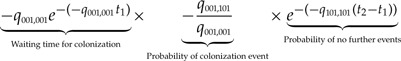
The probability of a particular biogeographic history can be calculated in a straightforward manner by assuming that the events of colonization and local extinction occur according to a continuous-time Markov chain (Ree et al. 2005). A continuous-time Markov chain is fully described by a matrix containing the instantaneous rates of change between all pairs of states (geographic ranges, in this case). This instantaneous-rate matrix, Q, has off-diagonal elements that are all ≥ 0 and negative diagonal elements that are specified such that each row of the matrix sums to 0. The elements of Q are parameterized by functions of θ, the parameter vector, according to some dispersal model, ℳ. The probability of a biogeographic history is obtained using the information on the position of colonization/extinction events on the tree and information from the instantaneous-rate matrix. Consider, for example, a case in which the process starts with a geographic range of 001 at one end of a branch, with a subsequent colonization of area one at time t₁ (i.e., changes from 001 → 101), and then remains in the geographic range 101 until the end of the branch at time t₂. The probability of this history is

There are an infinite number of biogeographic histories that can explain the observed geographic ranges. When calculating the probability of the observed geographic ranges at the tips of the phylogenetic tree, it is unreasonable to condition on a specific history of biogeographic change. After all, the past history of biogeographic change is not observable. Instead, the usual approach is to marginalize over all possible histories of biogeographic change that could give rise to the observed geographic ranges. The standard way to do this is to assume that events of colonization or local extinction occur according to a continuous-time Markov chain (Ree et al. 2005). Marginalizing over histories of biogeographic change is accomplished using two procedures. First, exponentiation of the instantaneous-rate matrix, Q, gives the probability density of all possible biogeographic changes along a branch

where y is the ancestral geographic range, z is the current geographic range, and t is the duration of the branch on the tree. The geographic-range transition probabilities obtained in this way marginalize over all possible biogeographic histories along a single branch, but do not account for the possible combinations of geographic ranges that can occur at internal nodes of the phylogeny. The Felsenstein (1981) pruning algorithm is typically used to marginalize over the different combinations of “states” (ancestral geographic ranges) at the interior nodes of the tree. Taken together, matrix exponentiation and the pruning algorithm comprise the conventional approach for calculating the probability of observing the geographic ranges at the tips of the tree while accounting for all of the possible ways those observations could have been generated under the model.

The dimensions of the instantaneous-rate matrix, Q, however, are , where , so the size of Q grows exponentially with respect to the number of geographic areas, N. Furthermore, computing the matrix exponential is of complexity ) (Golub and Loan 1983). Thus, for values of N ≥ 20, the number of computations required to exponentiate the rate matrix is quite large and computing the transition probabilities in this manner is intractable (Ree and Sanmartín 2009).

Statistical phylogenetic models encounter an analogous problem when modeling nucleotide evolution. As Felsenstein (1981) suggests, one might assume that each nucleotide site evolves under mutual independence to keep the state space small and amenable to matrix exponentiation. For biogeographic inference, however, the assumption of mutual independence would imply (implausibly) that the correlative effects between areas—such as geographic distance—are irrelevant to dispersal processes, which renders this assumption suitable only as a null model for testing the fitness of more plausible (e.g., distance-dependent dispersal) biogeographic models.

Our primary motivation here is to remove the computational constraint that precludes the elaboration of more complex (and realistic) biogeographic models. As a result of this focus, we leave the rigorous comparison of inference across alternative models and methods as an open topic for future study.

A Distance-Dependent Biogeographic Model

The instantaneous-rate matrix, Q, describes how the geographic range of a species can evolve through time. As with the formulation of Ree et al. (2005), we assume that in an instant of time only a single area can be gained or lost. In other words, each row of Q contains up to N positive, non-zero entries, which correspond to the rates at which any one of the N areas switches between absent and present (i.e., the N 0 → 1 and 1 → 0 positive entries of the row). Additionally, each row contains a single element on the diagonal of the matrix, defined as q_i,i = − ∑_i≠j q_i,j, which ensures that each row of Q sums to 0. The remaining entries in Q have a value of 0, as they entail an instantaneous change in geographic range involving two or more areas. This process corresponds to a dispersal–extinction (DE) model, which is somewhat simplified relative to the dispersal–extinction–cladogenesis (DEC) model (Ree et al. 2005), in that ancestral ranges are inherited identically. However, the current framework greatly expands the scope for the elaboration and inclusion of more diverse and realistic speciation scenarios.

We define a distance-dependent dispersal model, ℳ_D, where the rate of gaining a particular area (0 → 1) depends on the relative proximity of available areas to those currently occupied by a lineage. That is, the rate of colonizing a nearby area just outside the perimeter of the current geographic range should be greater than the rate of colonizing a relatively remote geographic area. The precise nature of the relationship between geographic distance and dispersal probability might be specified in numerous ways (see, e.g., Wallace 1887; MacArthur and Wilson 1967; Hanski 1998). Our distance-dependent model specifies a simple relationship in which the probability of dispersal between two areas is inversely related to the geographic distance between them.

Let q_y,z^(a) be the rate of change from the geographic range y to the geographic range z, where y and z differ only at the single area index a. Note that the rate function accepts any pair of bit vectors as arguments, allowing us to later assign configurations from x_i,•,k to y and z, x_i,•,k being the geographic range of species i at time τ_k⁽ⁱ⁾. Also, let λ₀ ∈ θ and λ₁ ∈ θ be the respective rates at which an individual area is lost or gained within a geographic range, and η(y,z,a, β) be a dispersal-rate modifier that accounts for correlative distance effects. We define the instantaneous dispersal rate as

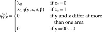(1)

and the distance-dependent dispersal-rate modifier as

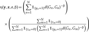(2)

where we define 1_{x=y} as the indicator function that equals 1 when both arguments are equal and 0 otherwise, and d(·) as the Great Circle distance between two geographical coordinates on the surface of a sphere, known by

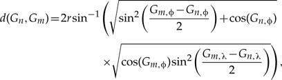where r is the radius of the sphere, and G_n is a vector with elements G_n,ϕ and G_n,λ that correspond to the latitude and longitude of the the centroid of discrete area n. Here, we take a sphere with r ≈ 6.37 ×10⁶ meters to approximate the size and shape of Earth.

Figure 2 will help develop intuition for how we model distance-dependent dispersal. In effect, the first term of η(·) computes the sum of inverse pairwise β-exponentiated geographic distances between the dispersal target, a, and all currently occupied areas of the geographic range. The second term normalizes the dispersal rate by the mean of all inverse pairwise geographic distances between all occupied–unoccupied area-pairs. This normalization ensures that the sum of dispersal rates with or without the distance-dependence modifier are equal, which helps identify and interpret parameters λ₁ and β. If η(·) = 1 or β = 0, then the rate of dispersal to area a equals the unmodified dispersal rate, λ₁. If β > 0, then the rate of dispersal to nearby areas is higher than that to more distant areas. Conversely, when β < 0, the rate of dispersal to more distant areas is higher than that to nearby areas. Finally, model ℳ_D is equivalent to ℳ₀ when β = 0.

Figure 2.

Cartoon of the computation of the distance-dependent dispersal-rate modifier, η(·). Here, we are interested in computing the rate of y = 1100 transitioning to z = 1101. The first term computes the sum of inverse distances raised to the power β between the area of interest (i.e., 4) and all currently occupied areas (i.e., areas 1 and 2). The second term then normalizes this quantity by dividing by the sum of inverse distances raised to the power β between all occupied–unoccupied area-pairs (i.e., the denominator), then multiplying by number of currently unoccupied areas (i.e., 2, the numerator).

Note that the rate of gain depends on the distance-dependent correlation function η(·), but the rate of loss does not, so the distance-dependent dispersal model is not time reversible when β ≠ 0. This fact has implications for evaluating the stationary frequency of geographic ranges at the root of the tree under this biogeographic model, which we detail below.

Sampling Biogeographic Histories

Our goal is to conduct inference under a dispersal model that captures the correlative effects of geographic distance between areas when N is large. For the computational reasons cited above, we cannot use matrix exponentiation to compute the likelihood under such a biogeographic model. Instead, we adapt a Bayesian data-augmentation approach that was introduced by Robinson et al. (2003) to model site-dependent protein evolution. Rather than analytically integrating over all possible biogeographic histories using matrix exponentiation, we numerically integrate over possible histories using data augmentation and MCMC.

We use the stochastic character-mapping algorithm described by Nielsen (2002) to sample biogeographic histories under the mutual-independence model, ℳ₀. This works by first sampling a set of geographic ranges for all internal nodes of the phylogeny and then sampling intermediate ranges over each of the branches connecting pairs of ancestor–descendant nodes. Upon completion, each branch is associated with a biogeographic history: the events comprising this history on each branch are ordered chronologically from past to present. Examples of such biogeographic histories are depicted in Figure 1b–d. We describe the process of sampling biogeographic histories in more detail below.

We first sample a set of geographic ranges for all M internal nodes from the joint posterior probability distribution of geographic-range configurations at the nodes. For tip nodes, we simply assign the observed species ranges. Next, we visit each individual branch in a pre-order traversal (moving from the root to the tips) of the tree. For each branch, we simulate a sequence of intermediate geographic ranges from the ancestral to the descendant node using rejection sampling; that is, the biogeographic history simulated along a branch must be consistent with the geographic ranges sampled/specified for the ancestor and descendant nodes of that branch. To do so, we first identify the initial geographic range at the ancestral node, the final geographic range at the descendant node, and the duration of the branch separating these two nodes. We then sample a history of dispersal events for each area under the mutual-independence model, ℳ₀, under a simple instantaneous-rate matrix for a single area

where λ₀^* and λ₁* are the per-area rate of loss/local extinction (1 → 0) and gain/colonization (0 → 1), respectively. To iteratively sample the biogeographic history for each area, j ∈ {1,...,N}, we initialize δ₀ = t_σ(i) and k = 1. Each iteration moves the process further along the branch by sampling a new event time δ from Q^*, updating δ₀ = δ₀ − δ, incrementing k, and inserting δ₀ into τ⁽ⁱ⁾ in sorted order as we go. Each event results in the state for area j changing to its complement (i.e., 0 → 1, or 1 → 0), which we record in the branch history, x_i,j,k. We continue to sample dispersal events until the time of the next event is younger than the age of the end of branch, δ₀ < t_i, whereupon we record the final event time as τ_F⁽ⁱ⁾ = t_i. Since time is exponentially distributed, the probability that any two areas undergo dispersal events at precisely the same instant occurs with probability 0, which is consistent with the one-change-at-a-time assumption of the model.

When the biogeographic history for area j is sampled, we check to make sure it matches the geographic ranges sampled at the nodes. Inconsistent histories are rejected and resampled for each area. Additionally, we reject and resample events that induce the forbidden extinction configuration. For models in which the per-site (per-area) state space is large, rejection sampling path histories can be computationally inefficient (c.f., Minin and Suchard 2007). This is not a concern in the present case, however, as the per-area state space is binary (i.e., 1 or 0 for presence/absence of a species in an area), so we opt for the simpler algorithm.

We iterate this process of simulating branch-specific biogeographic histories for the remaining branches, which we visit in a pre-order sequence. This results in τ⁽ⁱ⁾ for each branch, an ordered vector of event times across all N areas, enabling us to compute the model likelihood given a sampled biogeographic history.

Computing the Likelihood of Biogeographic Histories

Since we can compute the rate at which any area is gained or lost given the current geographic range, we can compute the likelihood of a sampled biogeographic history by adopting a “mechanistic” interpretation of the instantaneous-rate matrix, Q. In general, waiting times between events in a continuous-time Markov process are exponentially distributed: when the process is in state i, the next event will occur with an exponentially distributed waiting time, where the rate of the exponential is equal to the overall rate of leaving state i: q_i,i = − ∑_j≠i q_i,j. Moreover, the nature of the change at the next event is also specified by the instantaneous-rate matrix: the relative probability that the next event entails a change from state i to state j is p(i → j) = −q_i,j/q_i,i. Accordingly, the probability that the next event entails a change from state i to state j at time t is simply equal to the probability of any event occurring at time t times the relative probability that the event is a change from i to j.

In the present case, we let x_i,•,k = (x_i,1,k,x_i,2,k,...,x_i,N,k) be the state (sampled range) for lineage i at time τ_k⁽ⁱ⁾. Then, the probability that the next event is a the state change y → z at time t is the product of probability of the next sampled event occurring first among all possible events and the probability of any event occurring at time t, given as

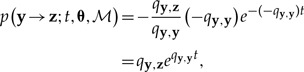(3)

and the probability that no event occurs in time t is given as

(4)

Note that the distance-dependent dispersal model defined in (1) depends on the superscript, (a), which indicates the single area that differs between ranges y and z. Here, we suppress the superscript in the interest of simplifying the notation. Changes between ranges that differ by more than one area have a transition rate of 0 (they are prohibited under the one-change-at-a-time model), so this summation requires only N computations.

The likelihood of the biogeographic history over all branches of the phylogeny is then simply calculated as the product of all stepwise likelihoods (Fig. 3),

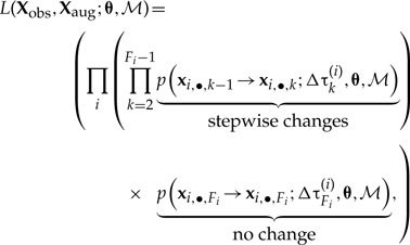(5)

where F_i = n(τ⁽ⁱ⁾) is the number of events on branch i, Δτ_k⁽ⁱ⁾ =(τ_k−1⁽ⁱ⁾ − τ_k⁽ⁱ⁾) is the temporal interval between events, and X_obs are the ranges observed at the tips.

Figure 3.

Cartoon of the likelihood terms. The biogeographic history for lineage i includes the lineage start at time τ₁⁽ⁱ⁾, an extinction event at area 2 at time τ₂⁽ⁱ⁾, a dispersal event into area 3 at time τ₃⁽ⁱ⁾, and the lineage end at time τ_F⁽ⁱ⁾, with all events laying within the time interval (3.2,9.3). The probability of a sampled geographic range at the start of the branch is conditioned on the previous (ancestral) geographic range and the time separating the geographic ranges, Δτ_k⁽ⁱ⁾ = τ_k−1⁽ⁱ⁾ − τ_k⁽ⁱ⁾. The likelihood is the product of the probabilities corresponding to each interval accounting for an area loss at time τ₂⁽ⁱ⁾, an area gain at time τ₃⁽ⁱ⁾, and no further changes occurring before the lineage terminates.

Markov Chain Monte Carlo

We can compute the posterior probability of a single sampled biogeographic history as

We approximate the joint posterior probability density of the biogeographic model parameters numerically using an MCMC algorithm. The general idea is to construct a Markov chain with a state space comprising the possible values for the model parameters and a stationary probability distribution that is the target distribution of interest (i.e., the joint posterior probability distribution of the model parameters). Draws from the Markov chain at stationarity are valid, albeit dependent, samples from the posterior probability distribution of the biogeographic parameters (Tierney 1994). Accordingly, parameter estimates are based on the frequency of samples drawn from the stationary Markov chain.

By repeatedly sampling dispersal histories via MCMC, we numerically integrate over X_aug,

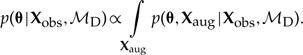To generate samples from this posterior, we rely on the Metropolis–Hastings algorithm (Metropolis et al. 1953; Hastings 1970). Below, we describe our MCMC proposals for an audience whom we assume has some familiarity with MCMC.

Proposing parameters.—Our method has two pairs of parameters for each area governing the rate at which it is added to or removed from the current biogeographic range: λ₀ and λ₁, which are used when computing the likelihood under the distance-dependent model; and λ₀^* and λ₁^*, which are used to sample biogeographic histories under the simpler mutual-independence model. All four rates must take on values > 0 and are distributed by half-Cauchy(0, 1) priors. We propose changes to the dispersal-rate parameters by first randomly selecting one of the four rates (uniformly with P = 0.25), then propose a new value for the selected rate parameter, x^′ = xe^ψ(u−0.5), where x is the current dispersal rate, x^′ is the proposed dispersal rate, ψ is a tuning parameter, and u ~ Uniform(0,1). The probability of accepting a proposed change to the dispersal-rate parameters, λ₀ and λ₁, under the distance-dependent model, ℳ_D, is calculated using the Metropolis–Hastings ratio

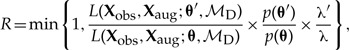where first term is the ratio of the likelihoods of the proposed and current states, the second term is the ratio of the prior probabilities of the proposed and current states, and the final term is the simplified Hastings ratio that describes the ratio of the proposal probabilities for the proposed and current states.

To improve acceptance rates for proposed dispersal histories under the mutual-independence model, ℳ₀, we infer (λ₀^*, λ₁*) ∈ θ^* by conditioning the likelihood on ℳ₀ instead of ℳ_D, yielding the Metropolis–Hastings ratio

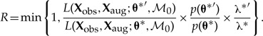We specify a Cauchy(0, 1) prior for the distance-power parameter, β, and propose new values , where ψ is a tuning parameter. The Metropolis–Hastings ratio to update β is

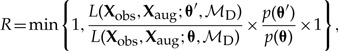where the Hastings ratio simplifies to 1 owing to the symmetry of the normal distribution. We used the Cauchy and half-Cauchy distributions as priors because they are weakly informative and fat-tailed, causing our inference to prefer parameter values near 0 while permitting parameters to take on large values should the data prove informative.

Proposing biogeographic histories.—To update biogeographic histories, we sample an internal node uniformly at random and a set of areas, , uniformly at random. We then propose a new biogeographic history by resampling the biogeographic histories for areas for incident branches using the stochastic-mapping approach described earlier.

The Metropolis–Hastings ratio for this proposal is

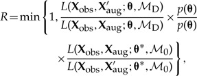where the first term is the likelihood ratio under the full model, ℳ_D, and the second term is the proposal-density ratio that accounts for the probability of sampling the proposed biogeographic histories under the sampling model, ℳ₀, using the sampling parameters, θ*. The parameters are not updated as part of this proposal, thus the ratio of prior probabilities may be safely omitted as it always equals 1.

Typically, the prior probability of each state (geographic range) at the root is equal to the corresponding stationary frequencies of the model. As mentioned above, our distance-dependent dispersal model is not time reversible, so we cannot approximate the stationary distribution by conventional means (c.f., Robinson et al. 2003). Instead, we leverage the fact that the stationary frequencies of states (geographic ranges) of a model can be approximated by simulating the continuous-time Markov process over a sufficiently long branch. Accordingly, we append a long stem branch to the root node, sample an ancestral “‘consensus” configuration as the ancestral state at the stem node, then simulate a biogeographic history along the stem branch that is consistent with the states at the beginning (stem node) and end (root node) of the stem branch. Thus, we simulate into the stationary distribution of geographic ranges under the distance-dependent dispersal model along the stem branch, and then sample from the approximated stationary distribution at the root node using the same proposal machinery as is used for any internal node.

Model Selection

The mutual-independence model, ℳ₀, is equivalent to the distance-dependent dispersal model, ℳ_D, when β = 0. Since ℳ₀ ⊆ ℳ_D, we compute Bayes factors for these nested models using the Savage–Dickey ratio (Dickey 1971; Verdinelli and Wasserman 1995), defined as

where P₀(β = 0|ℳ_D) is the prior probability and P(β = 0|λ₀,λ₁,x_obs, ℳ_D) is the posterior probability under the more general distance-dependent dispersal model, ℳ_D, at the restriction point β = 0, where ℳ_D is equivalent to the simpler mutual-independence model, ℳ₀. If the posterior probability under ℳ_D at β = 0 is significantly greater than the corresponding prior probability, then the Bayes factor supports ℳ_D (i.e., ℳ_D provides a better fit to the data). Since there is no analytical expression for the posterior probability, P(β = 0|λ₀,λ₁,x_obs, ℳ_D), we approximate its distribution using the non-parametric Gaussian kernel density estimation method provided by default in R(R Core Team 2012).

Data Analysis

Simulation study.—We simulated 50 dispersal data sets for each of eight values of β: 0, 0.25, 0.5, 1, 2, 3, 4, and 6. These data were simulated upon a geography with 20× 30 = 600 uniformly spaced discrete areas positioned over the Bay Area, California. Phylogenies were simulated under a pure birth process with rate 1, then scaled to have a height comparable to our empirical study phylogeny. Dispersal and extinction rates were also chosen to resemble the rates inferred from the empirical analysis, but scaled to account for the increased number of areas. We then ran independent MCMC analyses for each data set under the distance-dependent model. To identify the values of β that are indistinguishable from the mutual-independence model, we computed Bayes factors using the Savage–Dickey ratio for all posteriors inferred under the distance-dependent model.

We then quantified how well the posterior probabilities of dispersal histories correspond to the true biogeographic history known from the simulation. To do so, we compute the posterior probability of each area being occupied by each internal node for each analysis, then compute the sum of squared difference between each probability (0 ≤ P ≤ 1) and the corresponding true history (P = 0 or 1) recorded from the simulation. As this error term increases, the inferred ancestral ranges at nodes may be interpreted as less accurate.

Empirical study.—We applied our method to 65 species of the plant clade Rhododendron section Vireya, which are distributed throughout the Malesian Archipelago. We used the species distributions and 20 discrete areas of endemism reported by Brown et al. (2006), and the time-calibrated phylogeny reported by Webb and Ree (2012). To compute distances between areas, we used a single representative coordinate per area (depicted in Fig. 8a). To simplify the analysis, we hold the geography to be constant throughout time.

Figure 8.

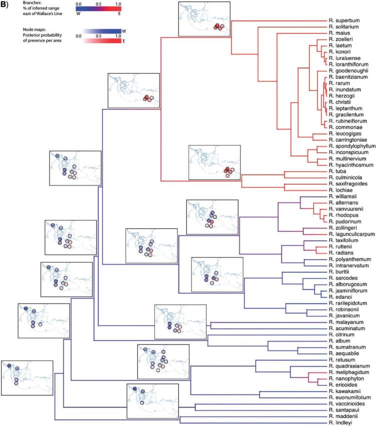
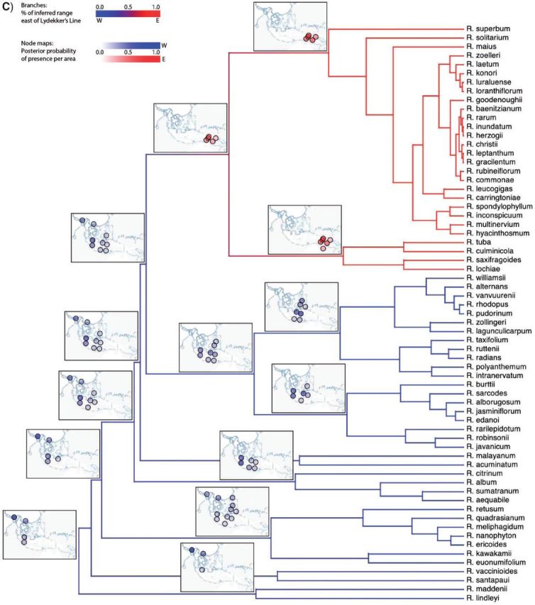
Biogeographic history of Malesian Rhododendron. A) The region was parsed into 20 discrete geographic areas following Brown et al. (2006), which straddle two important biotic boundaries—Wallace's and Lydekker's Lines. Each circle corresponds to a discrete area. Distances between these areas are based on a single coordinate for each area, indicated by an “x”. Posterior probability of being present in an area is proportional to the opacity of the circle. Occupied areas with posterior probabilities < 0.12 are masked to ease interpretation. Circles are shaded according to their position relative to Wallace's Line (B) or Lydekker's Line (C). Branches are shaded by a gradient representing the sum of posterior probabilities of being present per area for descendant–ancestor pairs. We infer a continental Asian origin for Malesian rhododendrons with multiple dispersal events across Wallace's Line (B) and a single dispersal event across Lydekker's Line (C).

Software configuration.—Each MCMC analysis of the simulated data ran for 10⁶ cycles, sampling parameters and node biogeographic histories every 10³ cycles. For the empirical data, we ran five independent MCMC analyses, each set to run for 10⁹ cycles, sampling every 10⁴ cycles. To verify MCMC analyses converged to the same posterior distribution, we applied the Gelman diagnostic (Gelman and Rubin 1992) provided through the coda package (Plummer et al. 2006). Results from a single MCMC analysis are presented. The methods described here have been implemented in BayArea, for which C++ source code is available for download at http://code.google.com/p/bayarea (last accessed June 28, 2013).

RESULTS

Simulation.—For 50 phylogenies of 20 tips and a fixed geography of 600 areas (see Methods section), we simulated 50 presence–absence data matrices for eight values of β: 0, 0.25, 0.5, 1, 2, 3, 4, and 6. Distributions of the mean posterior parameter values for the 8×50 MCMC analyses are shown in Figure 4. For β ≤ 3, the model was able to retrieve the true simulation parameters accurately, but this accuracy degraded for β ≥ 4 (see Discussion section).

Figure 4.

Distributions of means of posteriors of simulation study. Fifty data sets were simulated for each value of β ∈ {0,0.25,0.5,1,2,3,4,6} while λ₀ = 0.05 and λ₁ = 0.005 were held constant. For each set of 50 data sets, the mean of the posterior of each parameter was computed under the distance-dependent dispersal model. Distribution means are given by a bold line, while the 25th and 75th percentiles are given by the lower and upper edges of each box, called Q1 and Q3, respectively. The upper and lower whiskers indicate Q1 − IQR and Q3 + IQR, where IQR = 1.5 × (Q3 − Q1), and circles indicate outliers. The true parameter values are given by (A,B) the horizontal dashed line, and (C) the squares.

Figure 5 shows that Bayes factors consistently selected the correct model when data were simulated for β ≥ 1 and for β = 0. For data simulated when 0 < β < 1, we observed the greatest variance in the Bayes factor credible intervals. Data simulated under conditions in which distance had a weak effect on dispersal, i.e., β ≤ 0.25, were typically (and appropriately) indistinguishable from the mutual-independence model.

Figure 5.

Distributions of Bayes factors for the simulation study. Fifty data sets were simulated for each value of β ∈ {0,0.25,0.5,1,2,3,4,6} while λ₀ = 0.05 and λ₁ = 0.005 were held constant. Columns display the frequencies of strengths of support in favor of the distance-despendent dispersal model, where strengths of support correspond to the intervals suggested by Jeffreys (1961): Favors ℳ₀ on (−∞, 1); Insubstantial on [1, 3); Substantial on [3,10); Strong on [10,30); Very strong on [30,100); Decisive on [100,8). Each column corresponds to the strengths of support per 50 β-valued simulations. Bayes factors generally select the correct underlying model except for β = 0.25.

We then compared the true biogeographic history of each simulation to the corresponding posterior distribution of the sampled biogeographic histories. The sum of squared differences between posterior (estimated) and true (simulated) dispersal histories varied little for values of β ≤ 3, with slight elevation in error for β ≥ 4 (Fig. 6). The elevated error for large values of the distance-power parameter, β, may be caused by the underestimated parameter values, or it may be an artifact of our error metric; it carries an independence assumption, so it over-penalizes distance-dependent dispersal histories that contain an excess of “near misses” relative to “wild misses”.

Figure 6.

Errors for inferred dispersal histories of simulation study. The sum of squared differences between the posterior probability (i.e., 0 < P < 1) and the true history (i.e., P = 0 or P = 1) for each area and each internal node were computed per simulated data set. The box plots show the distribution of these sums for each batch of 50 simulated data sets per value of β ∈ {0,0.25,0.5,1,2,3,4,6}. Distribution means are given by a bold line, while the 25th and 75th percentiles are given by the lower and upper edges of each box, called Q1 and Q3, respectively. The upper and lower whiskers indicate Q1 − IQR and Q3 + IQR, where IQR = 1.5 × (Q3 − Q1), and circles indicate outliers.

Vireya.—Bayes factors strongly favor the distance-dependent dispersal model over the mutual-independence model to explain the biogeographic history of 65 rhododendron species in the section Vireya over 20 biogeographical areas throughout Malesia. The estimated maximum a posteriori (MAP) value of the rate of area loss was λ₀ = 0.13, the rate of area gain was λ₁ = 0.013, and the distance power was β = 2.65 (Fig. 7). Gelman–Rubin convergence values for λ₀, λ₁, and β between all pairs of MCMC analyses were < 1.1, which is consistent with all independent MCMC runs converging to the same posterior.

Figure 7.

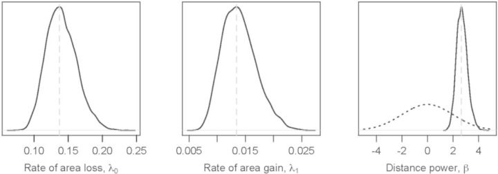
Marginal posterior densities for dispersal parameters from the Malesian Rhododendron data set. MAP values (dashed gray line) for the distance-dependent dispersal model parameters are A) λ₀ = 0.13, B) λ₁ = 0.013; and C) β = 2.65. The dotted black line corresponds to the prior, β ~ Cauchy(0,1). Note that the posterior probability of β = 0 is ~ 0, resulting in “Decisive” support (c.f., Jeffreys 1961) for the distance-dependent dispersal model over the mutual-independence model.

Figure 8 shows a summary of the inferred biogeographic history (Supplementary Fig. 1 shows the full history and observed ranges). The per-area posterior probabilities of the ancestral ranges strongly favor migration eastward into the Malesian Archipelago originating from Southeast Asia. The inferred biogeographic scenario—multiple independent dispersal events from the Sunda Shelf across Wallace's Line into Wallacea—is favored over that of a single dispersal event followed by pervasive extinction events (Fig. 8b). Lydekker's Line appears to be less permeable, with only a single lineage dispersing eastward from Wallacea across it onto the Sahul Shelf (Fig. 8c). An interactive animation of the ancestral range reconstruction is hosted at http://mlandis.github.com/phylowood/?url=examples/vireya.nhx (last accessed June 28, 2013).

Readers might naturally wonder how inferences under the current method compare to those based on alternative statistical biogeographic methods, such as the DEC model of (Ree et al. 2005). Despite their superficial similarities—both are likelihood-based methods that rely on continuous-time Markov models to describe the evolution of species geographic range—the methods differ to an extent that makes it difficult to draw any meaningful comparisons. Specifically, the two methods invoke models that differ in many respects (see Discussion section), and are implemented in different statistical frameworks (maximum likelihood vs. Bayesian inference).

DISCUSSION

Historical biogeography has begun the transition to explicitly model-based statistical inference (Ree and Sanmartín 2009; Ronquist and Sanmartín 2011). These methods describe the biogeographic process by means of continuous-time Markov chain that models the colonization of—and extinction within—a set of discrete geographic areas, and calculate the likelihood of the observed species geographic ranges at the tips of the tree using matrix exponentiation (to integrate over possible biogeographic histories along branches) and Felsenstein's pruning algorithm (to integrate over possible ancestral ranges at the interior nodes of the tree). Although this is a vigorous area of research, reliance on matrix exponentiation ultimately entails serious computational constraints that limit both our ability to develop more elaborate and realistic biogeographic models and to apply these methods to more complex and typical empirical problems.

We offer a Bayesian solution to this constraint that relies on data augmentation and MCMC to numerically integrate over biogeographic histories to estimate the joint posterior probability of the parameters given the data. The primary implication of this approach is a substantial increase in the number of discrete areas that can be accommodated—by approximately two orders of magnitude. Moreover, we propose a simple distance-dependent dispersal model in which rates of area colonization are a function of geographic distance. The nature and strength of the distance effect on rates of colonization are governed by the distance-power parameter, β. When β > 0, dispersal events over long distances are penalized, whereas long-distance dispersal events are favored when β < 0. Importantly, when β = 0, the distance-dependent dispersal model collapses to the simpler mutual-independence model, and so ℳ₀ ⊆ ℳ_D. Because the models are nested, we can use the Savage–Dickey density ratio to compute Bayes factors for robust model selection.

In the remainder of this section, we attempt to develop an intuition regarding the behavior of this new biogeographic approach, describe some of the benefits and limitations of the current implementation, and consider how this approach might be profitably extended.

Exploring the behavior of the Bayesian biogeographic framework—We explored the statistical behavior of our biogeographic model and inference framework via analyses of simulated and empirical data. The simulation study comprised 50 dispersal data sets for 20 taxa and 600 areas that were simulated under each of eight strengths of distance effects, β: 0, 0.25, 0.5, 1, 2, 3, 4, and 6. For β ≤ 3, we were generally able to infer the true parameters. However, estimation accuracy begins to suffer when β ≥ 4, resulting in all parameters being slightly underestimated. Estimation accuracy is also high for inferences based on time-series data simulated under large β values, so the poor accuracy appears to emerge from the phylogenetic structure underlying the data. Although values of β ≥ 4 are greater than those we have inferred from empirical data, we advise increased caution should one's inference lie in this range of parameters. Using the Savage–Dickey ratio to compute Bayes factors, we found our ability to select the correct model was largely determined by the strength of β (Fig. 5). Future simulation studies should be extended to evaluate the effects of the phylogeny on inference (tree size, shape, uncertainty, etc.), the sensitivity of the model to various priors, and whether extreme parameter values introduce greater errors in ancestral geographic-range estimates.

As currently specified, the distance-dependent dispersal-rate modifier, η (·), only changes the dispersal rate per area, but not the summed rates of colonization and extinction over the geographic range. Accordingly, the equilibrium number of occupied or unoccupied areas for the geographic range is largely determined by the ratio of λ₁ and λ₀ (the per-area rates of colonization and extinction, respectively). When the geographic range involves occupation of a relatively small fraction of available areas—as occurs when the number of areas increases—the area colonization/extinction rate ratio becomes small in order to explain the low observed frequencies of area occupancy at the tips of the tree. In such situations, these relatively simple parameters may fail to fit the data well. Moreover, the size of inferred ancestral geographic ranges (in terms of the number of occupied areas) tends to be larger than those observed at the tips of the tree. This phenomenon is also characteristic of other parsimony- and likelihood-based biogeographic methods (e.g., Ronquist 1997; Ree et al. 2005; Clark et al. 2008; Buerki et al. 2011). One solution to both problems would be to favor sampled biogeographic histories with range sizes most similar to a carrying-capacity or range-size parameter.

We demonstrated the empirical application of our method with an analysis of the biogeographic history of 65 Vireya species distributed over 20 geographic areas across the Malesian Archipelago (Brown et al. 2006). Bayes factors strongly favored the distance-dependent model, with a MAP estimate of β = 2.65 (Fig. 7). Brown et al. offered two hypotheses for the origin of Rhododendron: as an old genus that arose in Australia, or as a young genus that arose in Asia. Under our model, the posterior of sampled biogeographic histories at the root of the tree suggests that Asia is the most probable point from which the genus entered the Malesian archipelago (Fig. 8).

The inferred biogeographic history of Vireya involves several episodes of dispersal across Wallace's Line and a single episode of dispersal across Lydekker's Line (Fig. 8b,c). We note two points regarding these dispersal events. First, the earliest dispersal across Wallace's Line and the single dispersal across Lydekker's Line appear to have occurred at approximately the same time. Adopting 55 Ma as the crown age of the Rhododendron phylogeny (Webb and Ree 2012) implies that these dispersal events occurred in the Late Eocene (~ 40 Ma). At that time, many of the discrete areas in the western part of the Malesian Archipelago collectively formed a contiguous, emergent terrestrial region, Sundaland (Lohman et al. 2011), which may have facilitated the easterly dispersal of Vireya species from their ancestral range in continental Asia across Sundaland. Moreover, the eastern border of Sundaland was not yet bounded by a contiguous deep oceanic trench, which may have facilitated the continued easterly dispersal from Sundaland into Wallacea (across Wallace's Line) and eastward out of Wallacea (across Lydekker's Line) into the eastern region of the Malesian Archipelago.

The second point pertains to the apparent prevalence of dispersal events across Wallace's line. The origin of Vireya in continental Asia may have permitted the accumulation of greater species diversity throughout Sundaland, west of Wallacea. This would have established a greater species-diversity gradient across Wallace's line than that for Lydekker's line. Consequently, there may have been more opportunity for species to disperse across the western boundary (Wallace's line) into Wallacea than there has been for species to disperse across the eastern boundary (Lydekker's line) out of Wallacea.

Advantages and limitations of the Bayesian biogeographic method.—Increasing the number of areas offers several benefits. The most obvious, of course, is the ability to increase the geographic resolution of biogeographic inference. As we increase the number of areas, discrete biogeography better represents the continuous features of Earth. As an example, for a clade of terrestrial species that collectively share a global distribution, a statistical biogeographic analysis would want to discretize the (approximately) 1.5×10⁸ km² of terrestrial space into a meaningful number of areas. With ~15 areas (the previous limit), the average area would be comparable in size to Canada (∼10⁷ km²); for ~1500 areas (manageable under the current approach), the average area would be comparable to the size of Ohio (≈ 10⁵ km²).

Second, biogeographic areas have traditionally been defined on the basis of empirical analysis. For systems that do not have well-defined biogeographic areas, our method allows the biogeographer to agnostically define areas according to a grid, as was done in our simulation study. By studying the congruence between posteriors of dispersal histories for alternatively discretized geographies, one could determine the optimal discretization for a particular system, including both the number and shapes of areas. For example, a researcher with intimate knowledge of a study system may derive a geographic discretization that produces radically different ancestral-range estimates than those based on a uniformly gridded discretization. Such a scenario suggests that one of the two discretizations does not properly “weight” the importance of certain geographic areas when inferring the biogeographic history.

Although it has benefits, the ability to increase the geographic resolution also raises new issues. At highly resolved spatial scales, for example, it may become more difficult to accurately specify the occupancy of species within individual cells of the geographic grid. Inference under our model conditions on the biogeographic ranges of species at the tips of the tree, and errors in specifying these ranges are likely to lead inference astray. One solution to this issue would be to use species-distribution models to first predict the geographic ranges of species, and then treat these estimated ranges as the observed species' geographic ranges (analogous to the conventional practice of treating a multiple-sequence alignment—an inference predicted from the raw data—as the observations used to infer phylogeny).

Extending the Bayesian biogeographic method.—The real benefit of the Bayesian framework is the tremendous extensibility that it affords. The current implementation makes various restrictive assumptions. For example, we assume a fixed (and known) tree, a static geological history, and a homogeneous environment. Below we touch briefly on three extensions that permit the approach to accommodate phylogenetic uncertainty, dynamic geological history, and environmental heterogeneity.

Our implementation assumes the phylogeny is known without error, a luxury that exists only under simulation. The most natural way to account for phylogenetic uncertainty would be to exploit a distribution of time-calibrated trees (estimated separately) as input for biogeographic inference. This approach is straightforward for methods that analytically integrate over biogeographic histories: simply define an MCMC proposal to draw a new tree from the marginal distribution of phylogenies. However, our model entails sampling biogeographic histories for a specific phylogeny. Accordingly, this extension will require the use of joint proposals for both biogeographic history and phylogeny that maintain good mixing of the MCMC (i.e., that ensure reasonable acceptance probabilities). This will be a challenging task.

It is important to emphasize that our empirical analysis was conducted under the assumption of a static geological history: we explicitly ignore the substantial effects of tectonic drift, changes in sea level, the formation of islands, etc. This greatly simplifies the analysis, of course, since biogeographic likelihoods are computed by conditioning on a single, static set of geographic distances. Ideally, paleogeographic reconstructions would inform the changing proximity of areas through time, and biogeographic inference would be computed by conditioning on a temporally dynamic geography. For example, consider the scenario in which two continents drift apart as time advances, which may be characterized as a time-ordered vector of maps, each map corresponding to the geography appropriate to each interval of geological time. Since our phylogeny is also measured in units of absolute time, the rates of gain and loss could easily be modified to condition on the relevant set of geographical coordinates. In the above scenario, distances between areas between continents would increase with time, so dispersal events between continents would become increasingly unlikely.

By adopting a DEC-like approach wherein cladogenesis events differ in pattern from anagenic dispersal and extinction events, our model would have to define transition probabilities between larger numbers of configurations; it is trivial to compute the model likelihood with a model that accounts for cladogenic events by conditioning on a single biogeographic history, but to numerically integrate over all possible cladogenic events via MCMC will require sophisticated proposal distributions.

Finally, we can incorporate other features of areas beyond their latitude and longitude—such as altitude, climate, and ecology—that may affect dispersal rates. Morphological evolution also has a noted role in biogeography—Bergmann's Rule (Freckleton et al. 2003), traits that effect long-distance dispersal ability (Carlquist 1966), etc.—and could be jointly inferred along with dispersal patterns (Lartillot and Poujol 2011). These factors could variously be incorporated as parameters to construct a suite of candidate biogeographic models. As we demonstrated for exploring the effect of geographic distance, marginal likelihoods under different biogeographic models could then be computed and Bayes factors used to identify biogeographically important model components.

Noting the simplicity of their biogeographic model, (Ree et al. 2005) drew an analogy to the earliest work on probabilistic models of molecular evolution—the (Jukes and Cantor 1969) model. Although it admittedly offered a rudimentary description of the process, this first model nevertheless provided a critical proof of concept that the problem could be profitably pursued in a statistical framework. To extend this analogy, we believe the current contribution resembles the subsequent paper by (Felsenstein 1981), in which he proposed the pruning algorithm that—by virtue of conferring a tremendous increase in computational efficiency—heralded an era of progress in developing stochastic models for the analysis of DNA and amino acid sequence data that has been one of the great success stories in evolutionary biology. We are hopeful that the small steps made here will precipitate a similar era of productivity in the field of biogeographic inference that will enhance our ability to make progress on this important problem.

SUPPLEMENTARY MATERIAL

Supplementary Material, including Supplementary figures and Vireya data files can be found at http://datadryad.org and in the Dryad data repository (DOI:10.5061/dryad.8346r; last accessed June 28, 2013).

FUNDING

This research was supported by the National Science Foundation (NSF) [DEB 0445453 to J.P.H.; DEB 0842181, DEB 0919529 to B.R.M.] and the National Institutes Health (NIH) [GM-069801 to J.P.H.].

REFERENCES

- Brown G., Nelson G., Ladiges P.Y. Historical biogeography of Rhododendron Section Vireya and the Malesian Archipelago. J. Biogeogr. 2006;33:1929–1944. [Google Scholar]
- Buerki S., Forest F., Alvarez N., Nylander J.A.A., Arrigo N., Sanmartín I. An evaluation of new parsimony-based versus parametric inference methods in biogeography: a case study using the globally distributed plant family Sapindaceae. J Biogeog. 2011;38:531–550. [Google Scholar]
- Carlquist S. The biota of long-distance dispersal: I. Principles of dispersal and evolution. Q. Rev. Biol. 1966;41:247–270. doi: 10.1086/405054. [DOI] [PubMed] [Google Scholar]
- Clark J.R., Ree R.H., Alfaro M.E., King M.G., Wagner W.L., Roalson E.H. A comparative study in ancestral range reconstruction methods: retracing the uncertain histories of insular lineages. Syst. Biol. 2008;57:693–707. doi: 10.1080/10635150802426473. [DOI] [PubMed] [Google Scholar]
- Dickey J. The weighted likelihood ratio, linear hypotheses on normal location parameters. Ann. Stat. 1971;42:204–223. [Google Scholar]
- Felsenstein J. Evolutionary trees from DNA sequences: a maximum likelihood approach. J. Mol. Evol. 1981;17:368–376. doi: 10.1007/BF01734359. [DOI] [PubMed] [Google Scholar]
- Freckleton R.P., Harvey P.H., Pagel M. Bergmann's rule and body size in mammals. Am. Nat. 2003;161:821–825. doi: 10.1086/374346. [DOI] [PubMed] [Google Scholar]
- Gallager R.G. Low-density parity-check codes. IRE Trans. Inform. Theory. 1962;8:21–28. [Google Scholar]
- Gelman A., Rubin D.B. Inferences from iterative simulation using multiple sequences. Stat. Sci. 1992;7:457–511. [Google Scholar]
- Golub G.H., Loan C.F.V. Matrix computations. Baltimore (MD): Johns Hopkins University Press; 1983. [Google Scholar]
- Hanski I. Metapopulation dynamics. Nature. 1998;396:41–49. [Google Scholar]
- Hastings W.K. Monte Carlo sampling methods using Markov chains and their applications. Biometrika. 1970;57:97–109. [Google Scholar]
- Jeffreys H. Theory of probability. Oxford: Oxford University Press; 1961. [Google Scholar]
- Jukes T.H., Cantor C.R. Evolution of protein molecules. In: Munro H.N., editor. Mammalian Protein metabolism. New York: Academic Press; 1969. pp. 21–123. [Google Scholar]
- Lartillot N., Poujol R. A phylogenetic model for investigating correlated evolution of substitution rates and continuous phenotypic characters. Mol. Biol. Evol. 2011;28:729–744. doi: 10.1093/molbev/msq244. [DOI] [PubMed] [Google Scholar]
- Lemey P., Rambaut A., Drummond A.J., Suchard M.A. Bayesian phylogeography finds its roots. PLoS Comput. Biol. 2009;5:e1000520. doi: 10.1371/journal.pcbi.1000520. [DOI] [PMC free article] [PubMed] [Google Scholar]
- Lemey P., Rambaut A., Welch J.J., Suchard M.A. Phylogeography takes a relaxed random walk incontinuous space and time. Mol. Biol. Evol. 2010;27:1877–1885. doi: 10.1093/molbev/msq067. [DOI] [PMC free article] [PubMed] [Google Scholar]
- Lemmon A.A., Lemmon E.M. A likelihood framework for estimating phylogeographic history on a continuous landscape. Syst. Biol. 2008;57:544–561. doi: 10.1080/10635150802304761. [DOI] [PubMed] [Google Scholar]
- Lohman D.J., de Bruyn M., Page T., von Rintelen K., Hall R., Ng P.K.L., Shih H.-T., Carvalho G.R., von Rintelen T. Biogeography of the Indo-Australian archipelago. Ann. Rev. Ecol., Evol. Syst. 2011;42:205–226. [Google Scholar]
- MacArthur R.H., Wilson E.O. The theory of island biogeography. Princeton (NJ): Princeton University Press; 1967. [Google Scholar]
- Metropolis N., Rosenbluth A.W., Rosenbluth M.N., Teller A.H., Teller E. Equation of state calculations by fast computing machines. J. Chem. Phys. 1953;21:1087–1092. [Google Scholar]
- Minin V.N., Suchard M.A. Counting labeled transitions in continuous-time Markov models of evolution. J. Math. Biol. 2007;56:391–412. doi: 10.1007/s00285-007-0120-8. [DOI] [PubMed] [Google Scholar]
- Nielsen R. Mapping mutations on phylogenies. Syst. Biol. 2002;51:729–739. doi: 10.1080/10635150290102393. [DOI] [PubMed] [Google Scholar]
- Plummer M., Best N., Cowles K., Vines K. CODA: convergence diagnosis and output analysis for MCMC. R News. 2006;6:7–11. [Google Scholar]
- R Core Team. R: a language and environment for statistical computing. Vienna, Austria: R Foundation for Statistical Computing; 2012. ISBN 3-900051-07-0. [Google Scholar]
- Ree R.H., Moore B.R., Webb C.O., Donoghue M.J. A likelihood framework for inferring the evolution of geographic range on phylogenetic trees. Evolution. 2005;59:2299–2311. [PubMed] [Google Scholar]
- Ree R.H., Sanmartín I. Prospects and challenges for parametric models in historical biogeographical inference. J. Biogeogr. 2009;36:1211–1220. [Google Scholar]
- Ree R.H., Smith S.A. Maximum likelihood inference of geographic range evolution by dispersal, local extinction, and cladogenesis. Syst. Biol. 2008;57:4–14. doi: 10.1080/10635150701883881. [DOI] [PubMed] [Google Scholar]
- Robinson D.M., Jones D.T., Kishino H., Goldman N., Thorne J.L. Protein evolution with dependence among codons due to tertiary structure. Mol. Biol. Evol. 2003;20:1692–1704. doi: 10.1093/molbev/msg184. [DOI] [PubMed] [Google Scholar]
- Ronquist F., Sanmartín I. Phylogenetic methods in biogeography. Ann. Rev. Ecol. Evol. Syst. 2011;42:441–464. [Google Scholar]
- Ronquist F. Dispersal-vicariance analysis: a new approach to the quantification of historical biogeography. Syst. Biol. 1997;46:195–203. [Google Scholar]
- Tierney L. Markov chains for exploring posterior distributions (with discussion) Ann. Stat. 1994;22:1701–1762. [Google Scholar]
- Verdinelli I., Wasserman L. Computing Bayes factors using a generalization of the Savage-Dickey density ratio. J. Am. Stat. Assoc. 1995;90:614–618. [Google Scholar]
- Wallace A.R. Oceanic islands: their physical and biological relations. Bull. Am. Geog. Soc. 1887;19:1–21. [Google Scholar]
- Webb C.O., Ree R.H. Historical biogeography inference in Malesia. In: Gower D., Johnson K., Richardson J., Rosen B., Ruber L., Williams S., editors. Biotic evolution and environmental change in Southeast Asia. Cambridge, UK: Cambridge University Press; 2012. pp. 191–215. [Google Scholar]