Optimization and variability of motor behavior in multi-finger tasks: What variables does the brain use?

Abstract

The neural control of movement has been described using different sets of elemental variables. Two possible sets of elemental variables have been suggested for finger pressing tasks: the forces of individual fingers and the finger commands (also called “finger modes” or “central commands”). In this study we analyze which of the two sets of the elemental variables is more likely used in the optimization of the finger force sharing and which set is used for the stabilization of performance. We used two recently developed techniques – the analytical inverse optimization (ANIO) and the uncontrolled manifold (UCM) analysis – to evaluate each set of elemental variables with respect to both aspects of performance. The results of the UCM analysis favored the finger commands as the elemental variables used for performance stabilization, while ANIO worked equally well on both sets of elemental variables. A simple scheme is suggested as to how the CNS could optimize a cost function dependent on the finger forces, but for the sake of facilitation of the feed-forward control it substitutes the original cost function by a cost function, which is convenient to optimize in the space of finger commands.

Introduction

The difficulty of a problem depends on the variables used to describe it. This is the case in physics, engineering, computer science, etc. The importance of the variables used by the brain to control the movement – the elemental variables – was first emphasized by Bernstein, 1967 and then thoroughly discussed afterwards (Gelfand & Tsetlin, 1961; Gelfand & Latash, 1998). For instance, evidence suggests that the brain unites muscles into groups and uses commands to the groups that lead to parallel scaling of muscle activation (Hughlings Jackson, 1889; reviewed recently by Tresch and Jarc, 2009). Each command defines a pattern of activation in several muscles and the overall behavior is shaped by the superposition of those patterns (d’Avella, Saltiel, & Bizzi, 2003; Ivanenko, Poppele, & Lacquaniti, 2004; Krishnamoorthy, Goodman, Zatsiorsky, & Latash, 2003). These patterns are often subject-specific and can vary from task to task within the same subject (Danna-Dos-Santos, Degani, & Latash, 2008). Different sets of the elemental variables can be involved in a hierarchical manner for any given task. For example, in grasping, at the higher level of the control hierarchy the brain operates with the variables produced by thumb and the virtual finger (the virtual finger represents the combined effect of the four fingers) while at the lower level the commands to the virtual finger are translated into the individual finger commands (Latash, Friedman, Kim, Feldman, & Zatsiorsky, 2010).

The abundance of the motor system gives the brain freedom to choose among many ways to achieve the same motor goal (Latash, 2012). The fact that the brain’s choice is rather reproducible suggests that the brain prefers some options over others; it may be assumed that it optimizes a certain criterion – a cost function. At the same time, the movements are executed in a noisy environment and hence they inevitably deviate from the optimal performance. In order to compensate for the deviations the brain has to implement stabilization mechanisms, which would shape the variability of the effectors to minimize the imprecision in important performance variables. Consequently, for the same task and the same level of control hierarchy the brain has to solve at least two problems: (1) optimize the distribution of the task among the effectors and (2) stabilize the task-relevant performance variables against motor variability. Though there are no doubts that different elemental variables can be employed by the brain for different motor tasks and at different levels of the control hierarchy, it is not clear whether the two problems – optimization and stabilization – are solved using the same elemental variables.

Finger pressing

The multi-finger force production is a convenient model problem to study the elemental variables used in optimization and stabilization of human movements (Li, Latash, & Zatsiorsky, 1998; Latash, Li, & Zatsiorsky, 1998). Usually the goal of the finger force production is to ensure certain values of total force and/or moment of force. They are called the performance variables, as they constitute the goals of the task (Latash, Scholz, & Schöner, 2002). Note that the number of individual finger forces is always greater than the number of the performance variables (Zatsiorsky & Latash, 2008) and hence there exist abundant combinations of finger forces that solve the task. The CNS may benefit from such abundance (Latash, 2012) by optimizing a certain cost function and shaping the variability of the individual finger forces to reduce the variability of the performance variables. In the current study we will use a finger pressing task to analyze the underlying elemental variables.

The most obvious candidates for the role of the elemental variables are the finger forces themselves. Yet it is not clear to what extent the finger forces can be produced independently. The evident fact that one cannot flex a finger while keeping other fingers perfectly immobile also has its reflection in the force production and is called enslaving (Zatsiorsky, Li, & Latash, 1998, 2000).

A hypothesis has been suggested (Li, Zatsiorsky, Latash, & Bose, 2002; Zatsiorsky et al., 1998) that the central controller does not operate with the individual finger forces but instead it assigns hypothetical finger commands, or modes, which are then distributed among the fingers. Li, Zatsiorsky, et al., 2002 suggested an algorithm that enables determining the relationship between the hypothetical finger commands and the actual forces of the fingers.

Hence, there are two candidates for the role of the elemental variables underlying the finger force control: the finger forces themselves and the hypothetical finger commands. A priori it is difficult to say which of them is more likely to be used in stabilization and/or optimization. To address this question we will use two complementary methods – the analytical inverse optimization (ANIO; Terekhov, Pesin, Niu, Latash, & Zatsiorsky, 2010; Terekhov & Zatsiorsky, 2011) and uncontrolled manifold analysis (UCM; Scholz & Schöner, 1999; Latash, Scholz, & Schöner, 2002).

The ANIO method allows for the identification of an unknown cost function from the experimental data under the assumption that this cost function is additive with respect to known elemental variables, i.e. it can be represented as the sum of individual cost function of each variable. The UCM method evaluates coordination among the known elemental variables by comparing two components of variance within the space of elemental variables, one of them has no effect on the performance (variance within the UCM), while the other does (variance orthogonal to the UCM).

These two methods were successfully used together to describe the properties of the finger force distribution in pressing task (Park, Zatsiorsky, & Latash, 2010; Park, Sun, Zatsiorsky, & Latash, 2011; Park, Singh, Zatsiorsky, & Latash, 2012), yet in all of these studies the finger forces were assumed as the elemental variables. In the current study we will use these two techniques to judge which of the two candidates – finger forces or finger commands – are more likely to be the elemental variables for the optimization (ANIO) and stabilization (UCM).

On the coordinate sensitivity of ANIO

The ANIO method enables the reconstruction of an unknown cost function from the experimental observations given that the function is additive with respect to certain known elemental variables. The function J(x₁, … , x_n) is said to be additive (also additively separable, or just separable) if it has the form

$$J(x_1,\dots ,x_n)=g_1\left(x_1\right)+\cdots +g_n\left(x_n\right).$$

The additive cost functions have a useful feature that their optimization represents a significantly simpler problem than that of a function possessing no such structure (Floudas & Pardalos, 2009). We assume that, when dealing with optimization, the CNS favors the elemental variables, with respect to which the cost function is additive. The ANIO method allows us to check if the data were produced by a cost function additive with respect to certain variables. A brief description of the method can be found in Appendix AError Reference source not found., for more details see (Terekhov, Pesin, et al., 2010).

Note that not every cost function is additive with respect to a given set of variables (see Appendix A, or Xu, Terekhov, Latash, & Zatsiorsky, 2012, for a counterexample) and hence the same cost function is very unlikely to be additive with respect to two different sets of variables, such as finger forces and commands. To illustrate this consider a trivial example of a cost function additive for two finger forces:

$$J(F_1,F_2)=k_1{F}_1^2+k_2{F}_2^2,$$

where k₁ and k₂ are positive coefficients.

Let us build artificial elemental variables

$$\begin{array}{cc}\hfill v_1=& 0.55F_1+0.45F_2,\hfill \\ \hfill v_2=& 0.45F_1+0.55F_2.\hfill \end{array}$$ (1)

The same cost function written for these variables takes the form

$$J(v_1,v_2)=(30.25k_1+20.25k_2)v_1^2+(30.25k_1+20.25k_2)v_2^2+24.75(k_1+k_2)v_1{v}_2.$$

The function J evidently cannot be additive with respect to v₁ and v₂, because this would require that k₁ = −k₂, which is impossible to satisfy for positive coefficients k₁ and k₂.

The ANIO method attempts to fit the experimental data with a cost function additive with respect to the chosen elemental variables and it returns an indicator of the quality of the fit. By applying ANIO to the finger force data and using finger forces or finger commands as elemental variables we can check which of these two sets of variables yields better fit.

In the previous studies (Terekhov, Pesin, et al., 2010; Park et al., 2010) ANIO produced very high quality of fit when the finger forces were used. As it is rather unlikely that the same data set can be explained by a cost function additive with respect to two different sets of variables we hypothesize that the finger commands must yield lower quality of the fit than the finger forces (Hypothesis 1).

On the coordinate sensitivity of UCM

The UCM analysis can be used to evaluate the degree of coordination, or synergy, between multiple elements involved in the same task. The evaluation is made by comparing the experimentally observed variability of the performance variables with the variability they would have if every element acted independently.

The resulting score depends on the selected elements (Sternad, Park, Müller, & Hogan, 2010). As stronger coordination is more likely to be observed for the elemental variables than for any others, the UCM can be used to judge which of two sets of variables – finger forces or finger commands – are more probably used in synergies stabilizing specific performance variables.

In order to illustrate this idea consider a simple problem of stabilization of total pressing force produced by two fingers:

$$F_1+F_2=F_{\mathit{total}}.$$

Let us assume that experimentally measured forces are distributed in the ellipse shown in Figure 1Error Reference source not found.A. It is clear from the figure that the forces are coordinated to minimize the variance of the performance variable, F_total.

Figure 1.

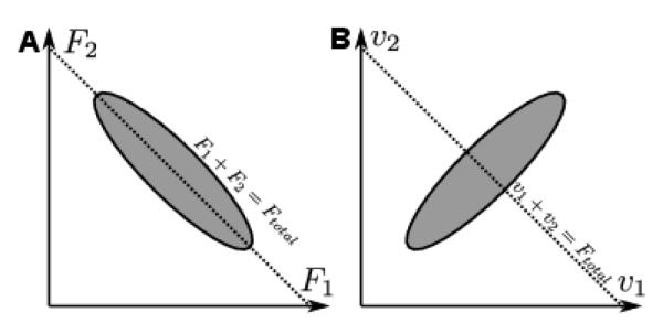
The coordinate sensitivity of the UCM analysis. A: the inter-trial variance of two finger forces, F₁ and F₂, in a thought experiment involving the total force stabilization. The resulting ellipse is elongated along the UCM (dashed line), which corresponds to all finger forces whose sum equals the target value. B: the variance of the same data set as in A, but plotted in artificially constructed coordinates, v₁ and v₂ (see the text); the variance ellipse is oriented orthogonal to the UCM (dashed line). This example shows how the same data can be interpreted as stabilizing or destabilizing certain performance variable depending on the choice of the elemental variables. This property of the UCM analysis provides means for testing the plausibility of certain elemental variables being used by the CNS in the performance stabilization process.

The same task formulated for the variables v₁ and v₁ defined in (1) is described as:

$$v_1+v_2=F_{\mathit{total}}.$$

Note that we deliberately defined the variables v₁ and v₂ in (1) so that the expression for the force stabilization task would be the same for both these variables and forces. Figure 1Error Reference source not found.B shows the same data as in Figure 1Error Reference source not found.A but plotted in the coordinates of v₁ and v₂. Clearly, the distribution in Figure 1Error Reference source not found.B shows no stabilization of F_total.

Thus the same data can be interpreted differently, depending on which variables are chosen as elemental. It is unlikely that the CNS would coordinate the elemental variables so that they would destabilize the desired performance, and hence when the choice is to be made between F₁, F₂ or v₁, v₂ it seems more reasonable to assume that F₁ and F₂ are the elemental variables.

This example shows that the UCM method can be used to evaluate the are the elemental variables. likelihood of certain variables being used as elemental variables for the performance stabilization. As the effect of enslaving provides strong evidence that the finger forces control is mediated by the finger commands, we expect that the UCM analysis will elicit significantly higher synergy indices for finger commands than for the finger forces (Hypothesis 2).

Methods

Subjects

Eleven right-handed males (age: 26.7±4.1 yrs, mass: 80.5±7.8 kg, height: 182.3±7.9 cm, hand length: 19.0±1.2 cm, and hand width: 8.4±0.3 cm; mean±SD across subjects) volunteered to participate in the current study. None of the subjects had a previous history of illness or injury that would affect the function of their upper arm, hand, or fingers. Hand length was measured from the tip of the middle finger to the distal crease at the wrist. Hand width was measured as the distance across metacarpophalangeal (MCP) joints of fingers 2 to 5, with the fingers in approximately neutral ab/adduction. Prior to performing the experiment subjects signed an informed consent form that was approved by the Office for Research Protections of the Pennsylvania State University.

Equipment

Pressing forces were measured using four uni-directional piezoelectric force transducers (208C02, PCB Piezotronics, Depew, NY). The transducers were rigidly fixed to metal rods mounted to an aluminum plate that was securely fastened to a table. The aluminum plate had slots so that the each of the individual rod-transducer couplings could be adjusted in the forward/backward direction in order to accommodate for different finger lengths of subjects.

Analog output signals from the transducers were sent to an AC/DC conditioner (5134B, Kistler, Amherst, NY, USA) then digitized with a 16-bit analog-to-digital converter (CA-1000, National Instruments, Austin, TX, USA). A LabVIEW program (LabVIEW Version 8.0, National Instruments, Austin, TX, USA) was written to control feedback and data acquisition during the experiment. The force signals were collected at 100 Hz. Post-data processing was performed using custom software written in Matlab (Matlab 7.4.0, Mathworks, Inc, Natick, MA).

Procedures

During the study, subjects were seated in a chair facing a computer screen. The right forearm rested on a padded support and the tip of each finger was positioned in the center of a force transducer. The distal interphalangeal (DIP), proximal interphalangeal (PIP), and MCP joints were all flexed in a posture that subjects felt was comfortable. A wooden block supported the palm of the hand. The block limited wrist flexion and supination/pronation of the forearm. The upper arm was positioned in approximately 45° shoulder abduction in the frontal plane, 45° shoulder flexion in the sagittal plane, and approximately 45° flexion of the elbow. The experiment consisted of three sessions, all of which were performed on the same day.

The goal of the first session was to determine the maximum voluntary contractions (MVCs) of the fingers to be later used in the computation of the finger commands. The experimental procedure is described in greater details in (Li, Latash, & Zatsiorsky, 1998; Li, Zatsiorsky, et al., 2002). The session required subjects to press with all one-, two-, three- and four-finger combinations (I, M, R, L, IM, IR, IL, MR, ML, RL, IMR, IML, IRL, MRL, and IMRL; where I stands for the index, M for the middle, R for the ring, and L for the little finger) to achieve their MVC. Subjects were asked to increase force in a ramp-like manner and to avoid a quick pulse of force production. They were required to maintain the force for a minimum of 1 s before relaxing. Sufficient rest was given between trials to avoid fatigue. The results obtained in this session were used for (a) determining the connection between finger forces and finger commands and (b) normalizing the target finger forces in the subsequent experimental sessions.

The purpose of the second experimental session was to collect the data necessary for the inverse optimization (ANIO) analysis. The detailed description of the experimental procedure can be found in (Park et al., 2010). Shortly, the session entailed producing a set of specified total force (F_total) and total moment (M_total) combinations while pressing naturally with all four fingers. The total orce produced by the fingers was computed as the sum of normal forces of the four fingers. The total moment produced by the fingers was computed as the moment produced about an axis passing mid-way between the M- and R-fingers. Subjects were required to produce both pronation (PR) and supination (SU) moments. The task set consisted of twenty-five combinations of five levels of F_total (20, 30, 40, 50 and 60% of individual MVC obtained in IMRL condition) and five levels of M_total (2PR, 1PR, 0, 1SU, and 2SU). In agreement with the previous study (Park et al., 2010) the moment levels were computed based on the 14% of the index finger MVC measured in its single-finger trial (MVC_I ):

$$M_{\mathit{total}}=0.14s_f{d}_I{\mathit{MVC}}_I$$

where d₁ stands for the moment arm of the index finger s_f and takes values −2, −1, 0, 1, and 2 corresponding to 2PR, 1PR, 0, 1SU and 2SU respectively.

The total moment produced by the fingers M was computed as

$$M=d_I{F}_I+d_M{F}_M+d_R{F}_R+d_L{F}_L$$

where F_j is the force of the corresponding finger and d_j is its moment arm with respect to the midline between middle and ring fingers. These value were set constant for all experiments: d_I =−4.5cm, d_M =− 1.5cm, d_R = 1.5cm, and d_L = 4.5cm.

Subjects performed five repetitions of each F_total and M_total combination. A total of 125 trials were performed (5 F_total levels × 5 M_total levels × 5 trials) in a randomized order. Each trial lasted for 5 s. Approximately 10 s of rest were given between the trials. In addition, several five-minute breaks were given during session two.

The purpose of the third session was to collect the data for performing the uncontrolled manifold (UCM) analysis. The session comprised additional 75 trials; 15 trials for each of the following conditions from the second session: 1) 20% F_total & 2PR M_total, 2) 40% F_total & 2PR M_total, 3) 20% F_total & 2SU M_total, 4) 40% F_total & 2SU M_total and 5) 40% F_total & 0 M_total. These conditions were selected in order to cover a broad range of experimental conditions while also minimizing fatigue of the subjects, which is why the 60% F_total condition was not included. Trials were performed exactly the same way as in the second session. They were organized in random blocks of the five conditions (i.e. all 15 trials of each condition were performed in a block of trials).

The three experimental sessions took between 1.5 to 2 hours. None of the subjects complained of pain or fatigue during or after the experimental sessions.

Data analysis

For all trials the force signals were filtered using a 4th order low-pass Butterworth filter at 10 Hz. In the first session, the peak force data were extracted for further analysis. For the second and third sessions, the individual finger force data from each trial were averaged over a 2 s time period in the middle of each trial (2- to 4-s windows), where steady-state values of total force and total moment were observed. For each trial the average finger force of each finger was extracted and used in the further analyses.

Computing the finger commands

As it was shown previously (Zatsiorsky et al., 1998; Gao, Li, Li, Latash, & Zatsiorsky, 2003; Danion, Schöner, et al., 2003) when the number of active (instructed) fingers is constant the dependency between the finger forces and finger commands is approximately linear:

$$\mathbf{F}=\Omega \mathbf{C},$$ (2)

where F = (F_I, F_M, F_R, F_L)^T is a 4×1 vector of finger forces, C = (C_I, C_M, C_R, C_L)^T is a 4×1 vector of finger commands, and Ω is a 4×4 inter-finger connection matrix.

The matrix Ω was computed from the MVC data (collected in the session 1) using the method developed by Li, Zatsiorsky, et al., 2002. Then for every vector of four finger forces collected in sessions 2 and 3 we computed the corresponding finger commands using formula (2).

Inverse optimization (ANIO)

The inverse optimization analysis was performed on the data obtained in the second experimental session. A brief description of the method is provided in Appendix A. A detailed description of the ANIO approach is available in (Terekhov, Pesin, et al., 2010; Terekhov & Zatsiorsky, 2011), a more brief description is also provided in (Park et al., 2010; Park, Sun, et al., 2011; Park, Zatsiorsky, & Latash, 2011; Park, Singh, et al., 2012; Niu, Latash, & Zatsiorsky, 2012; Niu, Terekhov, Latash, & Zatsiorsky, 2012).

The method assumes that the sought cost function is additive with respect to the chosen elemental variables and that the optimization is performed subject to linear constraints. Then it allows for the cost function determination from the experimental data. We used two sets of elemental variables: finger forces F and commands C. As it was shown in (Terekhov, Pesin, et al., 2010) the cost function, if exists, must be quadratic if the data distribution is close to planar, i.e. the data were confined to a two-dimensional hyper-plane. We estimated the planarity of the data both for forces and for commands using principal component analysis (PCA), using as an indicator the percentage accounted for by the two major principal components (PCs).

Following the convention used in the previous ANIO studies (Park et al., 2010; Park, Sun, et al., 2011; Park et al., 2011; Park, Singh, et al., 2012; Niu, Latash, & Zatsiorsky, 2012; Niu, Terekhov, et al., 2012) it was accepted that the experimental data were distributed in a plane if the two major PCs accounted for over 90% of the variance. This criterion was met for all subjects for forces and commands data. The two major components were said to define the experimental plane.

The cost function for the finger forces had the form

$$J_F\left(\mathbf{F}\right)=\sum _{j=I,M,R,L}(\frac{1}{2}{k}_j^F{F}_j^2+w_j^F{F}_j)$$

with the coefficients $k_j^F$ and $w_j^F$. This cost function was assumed to be optimized subject to the experimental constraints

$$\mathbf{DF}=\mathbf{d},$$ (3)

where

$$\mathbf{D}=\left(\begin{array}{cccc}\hfill 1\hfill & \hfill 1\hfill & \hfill 1\hfill & \hfill 1\hfill \\ \hfill d_I\hfill & \hfill d_M\hfill & \hfill d_R\hfill & \hfill d_L\hfill \end{array}\right),\mathbf{d}=\left(\begin{array}{c}\hfill F_{\mathit{total}}\hfill \\ \hfill M_{\mathit{total}}\hfill \end{array}\right)$$ (4)

The rows of the matrix D correspond to the constraints on the total force and total moment of force, respectively.

For the finger commands as elemental variables the cost function was

$$J_C\left(\mathbf{C}\right)=\sum _{j=I,M,R,L}(\frac{1}{2}{k}_j^c{C}_j^2+w_j^c{C}_j).$$ (5)

The expression for the constraints can be obtained by substituting (2) into (3):

$$\mathbf{D}\Omega \mathbf{C}=\mathbf{d}.$$ (4)

For both sets of elemental variables we normalized the coefficients so that ${\left(k_I^F\right)}^2+{\left(k_M^F\right)}^2+{\left(k_R^F\right)}^2+{\left(k_L^F\right)}^2=1$ and ${\left(k_I^C\right)}^2+{\left(k_M^C\right)}^2+{\left(k_R^C\right)}^2+{\left(k_L^C\right)}^2=1$.

We adopted the version of the ANIO algorithm from (Terekhov, Pesin, et al., 2010); it takes the experimental plane – the vectors of two major principal components (PCs) – and returns the coefficients of the cost function. In agreement with (Park et al., 2010) the average finger forces for each combination of target force and moment of force were computed prior to the principal component analysis. Since only few experimental planes can be fitted by an additive cost function, the algorithm returned coefficients correspond to the plane, which is as close as possible to the original plane and yet can be fitted by an additive cost function. The algorithm also returns the angle between these two planes, so called D-angle (Park et al., 2010). This angle reflects how well the data can be explained by a cost function with the chosen elemental variables.

Analysis of performance variability

The UCM analysis was used to describe the trial-to-trial variance quantitatively in every experimental condition. The details of the methods can be found elsewhere (Scholz & Schöner, 1999; Latash, Scholz, & Schöner, 2002). Shortly, it splits the entire trial-to-trial variance V_TOT of the elemental variables into two components by projecting it on two orthogonal subspaces. The first subspace – named UCM – is the null space of the task constraints, i.e. any variance of this subspace does not influence the performance variables (like F_total and M_total ). The second subspace is orthogonal to the UCM, and variance within this subspace has substantial effect upon the performance variables. The variances within each of these two subspaces are denoted as V_UCM and V_ORT respectively.

The main output of the UCM analysis is the index of variability

$$\Delta V=\frac{V_{\mathit{UCM}}∕(N_{\mathit{TOT}}-N_{\mathit{ORT}})-V_{\mathit{ORT}}∕N_{\mathit{ORT}}}{V_{\mathit{TOT}}∕N_{\mathit{TOT}}},$$

where N_TOT stands for the number of the elemental variables (four in this study) and N_ORT stands for the number of the performance variables (two, if both force and total moment of force are to be stabilized).

The index of variability shows whether the elemental variables are coordinated to stabilize the performance variables. When such coordination is present ΔV is positive; it has negative value if the elemental variables are coordinated to destabilize the performance variable and ΔV = 0 if there is no relevant coordination. The higher value of ΔV corresponds to stronger coordination, which according to our initial assumption is more likely to be present among the variables used in the performance stabilization.

The trials from the third experimental session as well as the five trials from the second session that matched the experimental conditions used in session three were combined for this analysis, giving a total of twenty trials per condition. The variance index ΔV was computed for two sets of hypothetical elemental variables: finger forces F and finger commands C, using the combinations of total force and total moment of force as performance variables (F_total&M_total). In addition to that ΔV was computed when only F_total or M_total was assumed to be the performance variable. This was done to ensure that the elemental variables are coordinated to stabilize both performance variables and not just one of them. If the latter were true, ΔV would be negative either for F_total or for M_total. The computational steps for the described analysis can be found in previous papers (Park et al., 2010; Park, Sun, et al., 2011; Park et al., 2011; Park, Singh, et al., 2012).

Statistics

In this study we investigate which of the two sets of elemental variables – finger forces or finger commands – is more likely to be used in optimization and stabilization of motor performance. Repeated-measures ANOVAs (RM ANOVAs) were used to check for which elemental variables ANIO yields a smaller D-angle and UCM yields higher ΔV. Analysis of the D-angle used one factor, ELEMENTAL VARIABLES (two levels, finger forces and finger commands). Analysis of ΔV used two factors: ELEMENTAL VARIABLES and PERFORMANCE VARIABLES (three levels, F_total, M_total and F_total&M_total). Wilcoxon’s signed-rank test was used to check if ΔV was significantly greater than zero.

Statistical analyses were performed using the Minitab 13.0 (Minitab, Inc., State College, PA, USA) and SPSS (SPSS Inc., Chicago, IL, USA). All the data was tested for sphericity and deviations were corrected using the Greenhouse-Geisser correction. A significance level was set at α = 0.05.

Results

Computing inter-finger connection matrices

In the first session the MVC finger forces were collected when subjects were instructed to press as hard as possible with all finger combinations. These data were used to determine the inter-finger connection matrices (see Methods). The inter-finger connection matrices displayed characteristics that were expected and agreed with previous results (Table 1Error Reference source not found.; Li, Zatsiorsky, et al., 2002; Zatsiorsky et al., 1998; Zatsiorsky, Latash, et al., 2004). The mean force deficit (±SD) of the I-, M-, R-, and L-fingers in the IMRL MVC task compared to the single finger MVC tasks were 39.9±22.6%, 27.8±17.9%, 37.9±17.0%, and 33.7±20.4%, respectively. Typical characteristics of enslaving were observed. In particular, the diagonal elements were positive for all subjects and in all cases the smallest diagonal element of a given subject’s matrix was larger than the largest off-diagonal element. Across subjects 23 of the 132 off-diagonal elements were negative (17.4%). In most occurrences of negative off-diagonal elements the absolute magnitude was less than 0.25 (16 of 23 occurrences).

Table 1.

The inter-finger connection matrices.

	Instructed finger
	I	M	R	L
I	16.16 (1.72)	1.16 (0.61)	0.28 (0.23)	0.41 (0.14)
M	1.44 (0.45)	15.34 (1.30)	1.11 (0.31)	0.00 (0.18)
R	0.47 (0.13)	1.98 (0.42)	11.32 (0.99)	1.09 (0.21)
L	0.31 (0.25)	0.57 (0.41)	1.67 (0.38)	11.36 (1.07)

Column headings are of the finger instructed to press. Mean values and standard error (in parentheses).

Exemplary finger commands are shown in Figure 2Error Reference source not found. as the functions of the target force and moment of force. The general pattern of commands agreed with the expected results: (1) the I-and M-finger commands were highest for the pronation effort tasks, (2) the R- and L-finger commands were highest for the supination effort tasks, and (3) for all fingers the commands increased as the force level increased. The group average commands for several of the moment and force combinations are presented in Table 2Error Reference source not found.. There were instances when commands were outside the 0 to 1 range. The percentage of values less than 0 was 0.1% and the percentage of values greater than 1 was 3.4% for the entire experimental data set of commands from session 2 (1375 data points; 11 subjects × 125 session).

Figure 2.

Exemplary data from the data set of one subject showing experimentally measured forces (column 1) transformed to finger commands (column 2) and the optimal finger commands (column 3) for each finger as plotted against the target force and moment of force.

Table 2.

Summary of finger commands.

Moment	Force (% MVC)	I	M	R	L
2PR	20	0.33 ± 0.04	0.31 ± 0.04	0.14 ± 0.02	0.06 ± 0.03
2PR	60	0.60 ± 0.05	0.81 ± 0.09	0.77 ± 0.06	0.41 ± 0.07
0	20	0.13 ± 0.02	0.27 ± 0.03	0.32 ± 0.03	0.18 ± 0.03
0	60	0.45 ± 0.04	0.72 ± 0.06	0.85 ± 0.03	0.60 ± 0.08
2SU	20	0.07 ± 0.01	0.14 ± 0.03	0.35 ± 0.03	0.50 ± 0.06
2SU	60	0.30 ± 0.03	0.64 ± 0.07	0.97 ± 0.07	0.79 ± 0.09

Mean finger command values for the boundary force and moment level combinations. Mean ± standard errors.

Notice that the middle finger commands were rather high in the supination task and the ring finger commands were high in the pronation task. The reason for such seemingly strange behavior is that, for a given moment of force, at high total force magnitudes using lateral fingers (I and L) with large lever arms would result in large moment magnitudes produced by those forces. To keep the total moment at a required magnitude, large moments in both pronation and supination would be needed (agonist and antagonist moment), which is a wasteful strategy. Using the middle fingers (M and R) with smaller moment arms allows to match the required moment of force without generating large antagonist moments.

Inverse optimization

In the second experimental session subjects were asked to press with their fingers in order to produce instructed combinations of total force and moment of force. The finger forces were recorded and then the finger commands were computed using inter-finger connection matrices as described in section.

According to the procedure of ANIO analysis at first we had to assure that the data has planar distribution. The planarity was estimated by means of principal component analysis (PCA). We found that data distribution was close to planar both for finger forces (96.2±0.6% of the total variance was accounted for by the first two PCs) and finger commands (94.1±0.7%). The fact that it was planar rather than linear was supported by the non-negligible second PC accounting for 23.8±7.3% of the total force and 27.9±8.3% of the total command variance (see Table 3Error Reference source not found. for more information). These numbers justify the choice of the quadratic cost functions in ANIO (for details see Terekhov, Pesin, et al., 2010). The first two PCs also define the experimental plane used in further ANIO analysis.

Table 3.

Summary of principal component analysis.

	PC1		PC2		PC1+PC2
	Median	Range (min, max)	Median	Range (min, max)	Median	Range (min, max)
Forces	72.63	(56.83, 80.76)	24.67	(13.57, 38.15)	96.67	(92.42, 98.26)
Commands	66.60	(53.53, 78.27)	29.13	(14.93, 39.82)	94.40	(90.47, 97.60)

Median and range of variance in PC1, PC2 and PC1 + PC2 are given.

After the planarity of the data distribution had been confirmed, ANIO analysis was used to determine the parameters of the cost function yielding the best fit of the experimental plane. Since not every experimental plane can be fitted with an additive cost function with chosen elemental variables, ANIO finds the closest plane that can be produced by an additive cost function. The closeness is measured by the dihedral angle (D-angle), which is the main output of ANIO used in the current study. A higher value of the D-angle signifies greater divergence between the experimental data and the distribution that could be expected if the data were generated by an additive cost function. Additionally, ANIO returns the coefficients of the cost function corresponding to the best-fit plane. For a cost function to be feasible, the second-order coefficients must be strictly positive.

For both sets of variables and in all subjects ANIO produced feasible cost functions as indicated by their strictly positive second-order coefficients. The average values of the coefficients are presented in Figure 3Error Reference source not found.A. The first-order coefficients are not presented here because they cannot be identified unambiguously (for details see Terekhov, Pesin, et al., 2010; Terekhov & Zatsiorsky, 2011).

Figure 3.

The results of ANIO analysis. A: the dihedral angles (D-angles) computed for finger forces and finger commands taken as elemental variables. The raw values are denoted with circles with thin lines showing the data belonging to same subject. The large squares connected with a thick line denote the group averages. B: the across-subjects average second-order coefficients of the cost functions with finger forces and finger commands taken as elemental variables. The coefficients have been normalized. Error bars are standard errors.

The D-angles were usually below 5° (Figure 3Error Reference source not found.B) suggesting that the experimental plane can be explained by additive cost functions both for finger forces and finger commands. For four subjects the D-angle was above 5° when computed for finger forces, and for three subjects this was the case in the space of finger commands. The D-angle fell out of the 5° range for the same three subjects for forces and for commands. The only exception is the subject for whom D-angle was 5.9° for forces and 4.4 degrees for commands. The average values of the D-angles nearly coincided: 4.46±1.21° for the force-based analysis and 4.39±0.89° for the command-based. No statistically significant difference was found (F(1,10) = 0.16, p > 0.700) between force- and command-based D-angles.

Uncontrolled Manifold Analysis

During the third experimental session subjects were asked to repeat certain combinations of total force and moment conditions so that the UCM analysis could be performed. This analysis was performed separately for a subset of {F_total; M_total} combinations with respect to three performance variables, F_total, M_total and F_total&M_total combined (see Methods). Across all subjects, conditions and analyses, the ΔV index was positive (Wilcoxon’s signed-rank test; p < 0.05). This can be interpreted as co-variation across trials of finger forces (commands) that stabilized each of the three performance variables for each of the studied {F_total; M_total} combination. Overall, the UCM analysis produced higher ΔV indices when the analysis was performed in the space of commands than in space of forces (see Figure 4Error! Reference source not found.). The effect of ELEMENTAL VARIABLE on z-transformed ΔV was highly significant (F(1,10) = 36.7, p < 0.001). The degree of coordination was typically the highest with respect to M_total, than to F_total, than to F_total&M_total:

$$\Delta V\left(M_{\mathit{total}}\right)>\Delta V\left(F_{\mathit{total}}\right)>\Delta V\left(F_{\mathit{total}}\&M_{\mathit{total}}\right).$$

This tendency was observed in all the experimental conditions and it was confirmed statistically (F(2,20) = 48.7, p < 0.001 for PERFORMANCE VARIABLE).

Figure 4.

Log-transformed normalized difference (ΔV_z) between variance within the UCM and variance orthogonal to the UCM with respect to: (A) total force and moment, (B) total force, and (C) total moment. Error bars are standard errors.

Discussion

First of all, we would like to note that the results obtained in the paper are consistent with the previous studies. The inter-finger connection matrices (Table 1Error! Reference source not found.), agree well with the previously published data (Danion, Schöner, et al., 2003; Li, Zatsiorsky, et al., 2002; Zatsiorsky et al., 1998, 2000). The same can be said about the ANIO and UCM results performed for the finger forces used as elemental variables (Park et al., 2010; Park, Sun, et al., 2011; Park et al., 2011; Park, Singh, et al., 2012; Latash, Scholz, Danion, & Schöner, 2001). Such a consistency of the findings strengthens our belief that the data obtained here for finger forces can be considered robust.

The current study aimed at answering the question of whether the brain uses the same set of elemental variables to optimize and to stabilize the motor behavior, or instead it uses two different sets, one for optimization and another one for the stabilization. We formulated two hypotheses: 1) the ANIO method will fail when applied to the finger force data using the finger commands as elemental variables and 2) the UCM will show higher degree of coordination for the commands than for the forces. The experimental data confirmed the second hypothesis only. To our surprise, ANIO worked almost equally well for the forces and the commands as elemental variables.

In what variables are synergies created?

For both forces and commands taken as elemental variables, the UCM analysis indicated that the majority of the variance was along the UCM (ΔV; Figure 4Error! Reference source not found.). This finding supports the notion that there was a multi-element synergy stabilizing the performance variables, total force, total moment of force and their combination. The synergy index ΔV was higher for finger commands than for the forces thus supporting the hypothesis that the synergies were based on the finger commands as elemental variables rather than finger forces.

The following explanation is offered as to why the finger commands taken as elemental variables outperformed the finger forces. Due to enslaving, finger forces display a certain degree of positive co-variation – this happens because in most cases all coefficients of enslaving matrices are positive. Thus, in the analysis with respect to F_total, ΔV could have been expected to be lower in the force space than in the command space because positive finger force co-variation contributes to F_totalvariance (V_ORT component in the UCM analysis).

The higher ΔV values in the analysis of M_total stabilization using commands are less trivial. Indeed, positive force co-variation due to the enslaving may have different effect on the total moment of force. The effect depends on particular patterns of enslaving. In an earlier study (Zatsiorsky et al. 2000), it has been shown that the enslaving patterns reduce the magnitude of the total moment produced by the fingers in pronation/supination. Given the importance of rotational hand actions in everyday life it is possible that the specific patterns of enslaving observed in healthy adults are optimal to ensure higher stability of the total moment of force.

The fact that the variance within the UCM was higher than the variance in the orthogonal sub-space suggests that the across-trial variability was attenuated by the negative co-variation within both sets of elemental variables and hence it cannot be explained by some kind of a “neuromotor noise” (Harris & Wolpert, 1998; Newell & Carlton, 1988; Schmidt, Zelaznik, Hawkins, Frank, & Quinn, 1979).

The higher value of ΔV in the command space may signal that the variance is reduced in task-relevant directions (smaller V_ORT ), but it could also reflect increase of variance in taskirrelevant directions (higher V_UCM ). Unfortunately, with the current analysis it is impossible to distinguish between the changes in these two potential contributors, because the variance computed in the space of forces cannot be directly compared to the one computed in the space of commands. Note that normalizing these values by the total variance V_TOT would not help because the resultant values would be nothing more but linear transformations of ΔV. For example, for normalized V_ORT computed for the force and moment of force performance variables is:

$$\frac{V_{\mathit{ORT}}}{V_{\mathit{TOT}}}=\frac{2-\Delta V}{4}$$

and similarly

$$\frac{V_{\mathit{UCM}}}{V_{\mathit{TOT}}}=\frac{2+\Delta V}{4}.$$

In what variables is optimization performed?

The results of the ANIO analysis are much less clear than the UCM results: against our a priori assumptions, the ANIO worked nearly equally well for the forces and for the commands.

For both sets of elemental variables the cost functions were quadratic. Note that the quadratic structure of the cost function was not assumed a priori, but follows from the planarity of the data distribution. Moreover, the planarity itself does not guarantee the existence of an additive cost function (see a counterexample in Xu et al., 2012). The possibility of a given plane to be explained by an additive cost function with selected elemental variables was measured by the D-angle. The D-angles were found to be rather small (typically <5°) and not significantly different between the command- and the force-based analyses, suggesting that for both sets of elemental variables the cost functions equally well capture the general tendency of the force sharing.

This finding is rather strange because, as it is discussed in previous papers (Terekhov, Pesin, et al., 2010; Niu, Latash, & Zatsiorsky, 2012), only a small percentage of experimental planes can be explained by additive cost functions with selected elemental variables. It is even more unlikely that the same plane can be explained by two cost functions with different sets of elemental variables. Yet this is exactly what our results show.

Can the result of ANIO analysis be coincidental?

One cannot exclude that, by pure coincidence, the experimental planes we obtained could be explained by cost functions with different elemental variables. It is important to have at least an estimate of the probability of such a coincidence. To do that we ran statistical simulations, described in Appendix B. At the first step, we estimated the probability that a random plane in the space of forces can be explained by an additive cost function with respect to the forces. For each subject we generated 10,000 random planes, such that they could explain all combinations of total force and total moment of force used in the experiments (with non-negative force values). We call these planes feasible. Then we computed the percentage of those planes, for which the D-angle was <5°and a hypothetical cost function corresponding to the plane that had positive second-order coefficients. We found that such planes constitute 10.3±6.2% of all feasible planes (the values denote average and standard deviation across all subjects). Hence, the probability that an arbitrary experimental plane can be explained by an additive cost function with accuracy corresponding to D-angle <5° is about 0.10. Note that this happened in all subjects, although the experimental planes differed among them. It is hard to estimate the joint probability because these events are not entirely independent, but neither are they imperatively connected. It is clear that the joint probability is below 0.10, so the latter can be used as a conservative estimate.

At the next step, we checked the probability of encountering an experimental plane that can be explained at the same time by a cost function additive with respect to the forces and by a cost function additive with respect to the commands. We repeated the same procedure as before, but now we computed the percentage of planes for which the same conditions were satisfied both for the forces and for the commands as the elemental variables. Such planes constituted just 5.0±1.3% of all feasible planes. This means that an arbitrary experimentally feasible plane has about 0.05 probability to be explainable by additive cost functions both for the forces and the commands taken as elemental variables. The experimental planes were different in all subjects, yet in all of them they had this property. Though it is hard to give an estimate of probability of such observation to occur by a pure chance, it is definitely below 0.05 and, thus it may reflect the underlying control mechanisms.

Interaction between the optimization and stabilization

The results of the current study are rather difficult to interpret. On the one hand, we found that the commands outperformed the forces in the UCM analysis and, thus are more likely to be employed in the stabilization aspect of the task. This assumption is also confirmed by the effect of enslaving itself, which suggests that the CNS has limited direct control of the individual finger forces (see review in Schieber & Santello, 2004).

Links between enslaving and synergy indices (ΔV ) are not trivial. For example, healthy older persons show decreased indices of enslaving and lower indices of both force- and moment-stabilizing synergies (Shinohara et al. 2003; Olafsdottir et al. 2007; Kapur et al. 2010). Both an increase and a decrease of enslaving under fatigue have been reported while multi-finger synergy indices are increased (Danion, Latash, Li, & Zatsiorsky, 2000; Singh, Varadhan, Zatsiorsky, & Latash, 2010; Singh, Zatsiorsky, & Latash, 2012). In neurological patients with subcortical disorders, enslaving indices are increased, while multi-finger synergy indices are significantly lower (Park, Lewis, Huang, & Latash, 2012; Park, Wu, Lewis, Huang, & Latash, 2012). These results suggest that there is no one-to-one link between enslaving and synergy indices. These observations emphasize the fact that the higher synergy indices computed in the space of commands to fingers, particularly those with respect to M_total, are not trivial consequences of positive enslaving.

On the other hand, ANIO worked equally well for the forces and the commands meaning that both coordinates are equally probable as the elemental variables for the optimization. Moreover, the probability of encountering the latter property by pure chance in all subjects is below 0.05. Though this observation deserves closer investigation, we can propose a simple provisional interpretation for it. Note that using additive functions is beneficial for the CNS as it simplifies the optimization problem (Floudas & Pardalos, 2009). Additive cost functions have a nice property that an increase of the cost due to a change in one elemental variable does not depend on the values of the other elemental variables. As a consequence, local search algorithms, like gradient descent, which may be employed by the CNS (Gelfand & Tsetlin, 1966; Ganesh, Haruno, Kawato, & Burdet, 2010), can be implemented in additive cost functions in a much easier way than in non-additive ones. So, the CNS may favor additive cost functions, and perform optimization in the coordinates, with respect to which the employed cost function is additive.

The interpretation we offer here is that the CNS might prefer to use the finger commands as the elemental variables both for optimization and stabilization, but at the same time it needs to optimize a cost function, which is additive with respect to the finger forces. The fact that the finger forces and patterns of their co-variation are adjusted to the expected force and moment of force in advance (Johansson & Westling, 1988; Olafsdottir, Yoshida, Zatsiorsky, & Latash, 2005; Shim, Park, Zatsiorsky, & Latash, 2006) suggests that the CNS determines the optimal solution in a feed-forward manner. While sensory information on finger forces is available to the CNS, it comes at a delay and may be of limited use for feed-forward optimization. So we suggest that, for a given task, the CNS develops a cost function formulated in terms of commands in such a way that its optimization also reduces the cost of a function that depends of finger forces, which may be more relevant to actual performance (cf. optimization approaches in Crowninshield & Brand, 1981; Alexander, 1999; Pataky, 2005; Prilutsky et al., 2009). In other words, to optimize the values additive with respect to the forces the CNS constructs intermediate cost function additive with respect to the commands, such that its minimization will at the same time bring a minimum to the cost function of forces. Such a two-level scheme will also allow the CNS to adopt mechanisms responsible for stabilization of important performance variables in the space of the finger commands.

A hypothetical scheme that implements the described processes is presented in Figure 5Error! Reference source not found.. This scheme is a slight modification of the central back-coupling (CBC) scheme introduced by Latash, Shim, Smilga, and Zatsiorsky, 2005. The tasks – the total force and the total moment of force – are transmitted into the performance variable stabilization neurons (PV ), which shape the variability of the feed-forward commands, produced by the C neurons. The C neurons project on PV stabilization neurons as a part of the stabilization loop, but at the same time they project onto the optimization neurons $J_i^{\prime }$, which in turn back-project on the C neurons, implementing the gradient descent optimization of the commands. Finally the outputs of the C neurons are mixed through the inter-finger connection matrix to yield actual finger forces.

Figure 5.

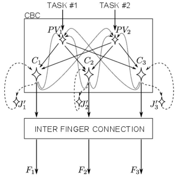
The hypothetical scheme of feed-forward control of the finger forces. The central controller assigns the values of two performance variables leading to signals to two PV neurons. Their outputs are shared among the C neurons, representing the finger commands. The stabilization of the performance variables is ensured by the back - coupling loop connecting the finger commands and the performance variables. At the same time another loop connects the C and $J_i^{\prime }$ neurons implementing an algorithm similar to gradient decent. Without the stabilization loop, the optimization would converge to an unconditional minimum of the cost function, e.g. to zero finger forces. The presence of the stabilization loop constraints the optimization so that the performance variables remain close to their desired values. Finally the outputs of the C neurons are combined together using inter-finger connection matrix to yield the finger forces.

Note that the optimization neurons $J_i^{\prime }$ are not directly involved in satisfying the task constraints; they try to bring commands to a minimum of the cost function. The action of these neurons is partly counterbalanced by the PV neurons, which stabilize the performance variables, by correcting the commands in the direction orthogonal to the UCM. Due to the combined functioning of these two mechanisms the conditional minimum of the cost function is achieved. Moreover, we can expect that the subjects will tend to deviate from the precise satisfaction of the task constraints towards the unconditional minimum of the cost function. Experimental investigation of this fact falls outside the scope of the current study.

This interpretation allows offering a likely answer to the question posed in the title of the study. The CNS probably uses the same elemental variables for the optimization and stabilization of the finger forces. In our study these elemental variables are the finger commands. This finding is not surprising for the stabilization, because the CNS has no direct access to the finger forces, only to the commands. In optimization, in turn, it seems that the CNS might minimize a cost function which is additive with respect to the forces, yet it substitutes that cost function with an intermediate cost function additive with respect to the commands. The benefits of such substitution are that the CNS can execute local search optimization in the variables it has direct access to – the commands – and the same mechanisms, which are used in stabilization, can also be employed in optimization to ensure the optimal values satisfy the task constraints.

Study limitations

We would like to mention a few limitations of the study. The first is that only one trial at each MVC condition was collected in order to avoid fatigue. Typically, several trials at each MVC task are collected and either averaged (Zatsiorsky, Gregory, & Latash, 2002) or the highest value taken as the true MVC force (Li, Zatsiorsky, et al., 2002). Inaccurate MVC forces could have a major effect on the inter-finger connection matrix computed from the neural network model. This would, in turn, cause the computed the finger commands to be inaccurate.

Here we assumed that the finger commands and finger modes are related through a linear equation when the number of actively instructed fingers is specified. There were no comprehensive studies of the links between finger forces and finger commands for tasks involving submaximal force and moment of force production. As a consequence, it may be that the relationship between the finger forces and finger commands is not perfectly linear and hence our estimates of the finger commands may differ from their “true values”.

Another limitation of the study is that it was assumed that the commands were between 0 and 1. Several of the computed finger commands were outside of this range for a few of the trials (both negative commands and commands greater than 1). This result is most likely in part linked to the limitation mentioned above (see details in Martin, Terekhov, Latash, & Zatsiorsky, 2012). It is also plausible that during some of the conditions the subjects were able to either decrease enslaving by activating extensor muscles or produced forces larger than they did in the MVC trials. The supination tasks may have caused subjects to produce quite large forces with their little fingers since the moment was scaled to the MVC of the index finger. Subjects with higher index to little finger MVC ratios may have been producing forces above the recorded little finger MVC.

The last limitation is that the range of target force and moment of force used, especially moments, only captured a small subset of what subjects were capable of producing. Using a greater range of target forces and moments could have resulted in a more accurate cost function approximation. However, we decided that the potential benefit of collecting a larger range of target forces and moments was outweighed by the extra fatigue these additional trials would have induced on subjects. We felt it was better to limit the total number of trials collected to obtain the most accurate set of forces over the space of task constraints used.

Appendix A

In this appendix we present a summary of the ANIO method and a brief description of the main theoretical results. ANIO is essentially based on the Uniqueness Theorem, which is presented first, and it exploits the duality between the planarity of the data and the quadratic nature of the underlying cost function, whose explanation goes next. Finally we present the method itself in the form it is used in the current study.

Uniqueness Theorem

Uniqueness Theorem states the sufficient conditions for a solution of the inverse optimization problem to be unique. Here we present the Uniqueness Theorem for the case of four variables and two constraints. The general case can be found in (Terekhov, Pesin, et al., 2010; Terekhov & Zatsiorsky, 2011).

Consider an additive cost function

$$J\left(\mathbf{x}\right)=\sum _{i=1}^4{g}_i\left(x_i\right)\to \mathit{min},$$ (7)

where g_i are scalar functions, x = (x₁, x₂, x₃, x₄)^T. The variables x can correspond to finger forces and finger modes. For the sake of convenience of notation here we use numerical and not literal indeces.

The cost function J is minimized subject to linear constraints

$$\mathbf{Dx}=\mathbf{d},$$ (8)

where D is a 2 × 4 matrix of constraints and d is a two-dimensional vector. In case when the problem is formulated for forces the matrix D is provided in (4).

We assume that every point x corresponds to a minimum of the cost function J under the constraints (8) for a certain vector d. Hence, at every point x the cost function J must satisfy the Lagrange principle, which in this case requires that:

$$\check{\mathbf{D}}{J}^{\prime }\left(\mathbf{x}\right)=0,$$ (9)

where J’(x) = (J’_x1, J’_x2, J’_x4)^T (prime symbol signifies derivative over the variable) and

$$\check{\mathbf{D}}=\mathbf{I}-{\mathbf{D}}^{\mathrm{T}}{\left({\mathbf{DD}}^{\mathrm{T}}\right)}^{-1}\mathbf{D},$$ (10)

I stands for a unit matrix.

Now let’s assume that there are two additive cost functions J₁(x) and J₂(x) producing the same set of experimental data X*. Evidently, both functions must satisfy Lagrange principle at every point of X*. We would like to know, what are the constraints of the experimental data X*, which would guarantee that the functions J₁ and J₂ coincide.

The answer is given by The Uniqueness Theorem. It states that if two nonlinear functions J₁(x) and J₂(x) satisfy the Lagrange principle for every point x in the set X* with the constraints matrix D and:

1. J₁ and J₂ are additive,

2. the data is distributed along a smooth two-dimensional surface X*,

3. the matrix Ď in (10) cannot be made block-diagonal by simultaneous reordering of the rows and columns with the same indices (such constraints are called non-splittable; Terekhov, Pesin, et al., 2010).

then:

$$J_1\left(\mathrm{x}\right)={\mathit{rJ}}_2\left(\mathrm{x}\right)+{\mathbf{q}}^T\mathbf{D}\mathrm{x}+\mathit{const}$$ (11)

for every x inside a hyper-parallelepiped surrounding the surface X* . The hyper-parallelepiped is defined as follows:

$$X_0^{\ast }=\{\mathbf{x}\mid \text{for every j exists}\tilde{\mathrm{x}}\in X^{\ast }:x_j={\tilde{x}}_J\}$$

r is a non-zero scalar value and q is an arbitrary four-dimensional vector.

The Uniqueness Theorem states that if any solution to the inverse optimization problem, J₁(x), is found then the true additive cost function J₂(x) is equal to J₁(x) up to multiplication by an unknown scalar r and adding an unknown linear terms q^TDx + const.

The conditions of the Uniqueness Theorem are impossible to satisfy exactly in real experiments, because it requires that: (1) the data form a two-dimensional surface, that implies infinite number of data points to be available, and (2) the data are precise, while in reality it is always disturbed by motor variability and measurement noise. Yet, as it has been shown in (Terekhov & Zatsiorsky, 2011) the cost function can be approximately determined even from imprecise and limited data if all other conditions of the Uniqueness Theorem are satisfied.

The link between the planarity of the data and quadratic cost functions

In the current study we assumed that the cost functions are additive quadratic polynomials. This assumption follows from the planarity of the data distribution and the Uniqueness Theorem. Indeed, a plane in four-dimensional space can be represented by a matrix equation:

$$\mathbf{Ax}+\mathbf{a}=0,$$ (12)

where A is a 4 × 2 matrix and a is a two-dimensional vector.

Assume that in the experiment the data were found to be distributed along the plane (12) and that these data correspond to a solution of the optimization problem with an unknown additive cost function J and linear constraints (8). We will show that then the cost function J must be quadratic.

Indeed, at its every point x the cost function J must satisfy Lagrange principle (9).

On the other hand, if the cost function is quadratic,

$$J\left(\mathbf{x}\right)=k_1{x}_1^2+\cdots +k_4{x}_4^2+w_1{x}_1+\cdots +w_4{x}_4,$$ (13)

then the equation (9) takes the form

$$2\check{\mathbf{D}}\mathbf{Kx}+\check{\mathbf{D}}\mathbf{w}=0,$$ (14)

where K is a diagonal matrix with the coefficients k₁, … , k₄ on the diagonal and w is a vector of the coefficients w₁, … , w₄.

Note that since the matrix Ď has rank two, the equation (14) also defines a plane. If there exist such coefficients k_i and w_i (k_i > 0 ) that the equations (12) and (14) define the same plane, then the function (13) is a possible solution for the inverse optimization problem (7), (8), (12). Hence, according to the Uniqueness Theorem the true cost function is also quadratic and coincides with J up to linear terms.

Now we check if for every plane (12) there exist such coefficients k_i and w_i that the plane can be represented as (14). If such coefficients do not exist, then the plane (12) cannot be explained by any cost function, additive with respect to x₁, … , x₄. The latter does not exclude that this plane can be explained by a non-additive cost function, or by a cost function additive with respect to another set of variables.

There are two reasons why the coefficients may not exist. First, it may happen that they exist, but some of k_i are negative. Second, it may happen that no coefficients at all can fit the plane (12) with equation (14). We will give additional explanations for the second possibility as it plays an important role in the current algorithm of the cost function determination. The algorithm itself will be presented in the next subsection.

For the planes (12) and (14) to coincide, the rows of matrix A must span the same vector subspace as the rows of matrix ĎK. The latter means that every row orthogonal to A must also be orthogonal to every row of ĎK, or

$$\check{\mathrm{A}}\mathbf{K}\check{\mathbf{D}}=0,$$ (15)

as Ǎ is a symmetrical matrix whose rows are orthogonal to the rows of A.

Since both matrices, Ǎ and Ď, have ranks equal to two, the equation 15 defines four linear equations on the coefficients k₁, … , k₄

$$\mathbf{Ek}=0,$$

where k is a vector of k₁, … , k₄ and E is 4×4 matrix produced from the elements of Ǎ and Ď. For the equation 15 to have a non-trivial solution (e.g. k_i ≠ 0) the determinant of E must vanish.

In four-dimensional space the orientation of the plane is defined by 5 parameters (just like it can be described by two parameters in three-dimensional space). In order for the plane to be explained by an additive cost function, these five parameters must be such that

$$\det \mathbf{E}=0.$$ (16)

Hence, not every plane in four-dimensional space can be explained by an additive cost function. Theoretical probability of getting such a plane by chance is zero. Since in the experiments the data are noisy, the plane cannot be determined precisely, and, thus, most probably it will not satisfy the equation (16). However, it may happen that a plane, which is very close to the one determined in the experiment, will do. Hence, we must search for such a plane, which is as close to the experimental plane as possible, and yet for which there exist coefficients k₁, … , k₄. This idea lies behind the ANIO algorithm described below.

ANIO algorithm

ANIO algorithm used in the current study searches for the parameters of a quadratic additive cost function that would fit the experimental data best. The details of the algorithm can be found in (Terekhov, Pesin, et al., 2010). The input to the algorithm is the experimental plane in the form (12), which we defined by the two largest eigenvectors of the data co-variation matrix and the vector of the data barycenter. The algorithm searches for the coefficients k_i, w_i of a cost function (13), such that the dihedral angle (D-angle) between planes (12) and (14) is minimized. The D-angle is computed using Matlab function subspace, the minimization is performed using fminunc function of Matlab Optimization Toolbox. The parameters w_i are determined form the data barycenter. We assume that the algorithm succeed if all coefficients k_i are positve. In this case the D-angle can be used as a measure of how likely it is that the data are generated by a cost function additive with respect to selected variables.

Note that according to Uniqueness Theorem the vector w cannot be determined uniquely. In the current paper we choose the vector w which would have the minimal length among all possible vectors. As it is shown in (Terekhov, Pesin, et al., 2010), such vector w can be computed as:

$$\mathbf{w}=-\mathbf{DK}\overline{\mathbf{x}},$$

where $\stackrel{‒}{\mathbf{x}}$ is the barycenter of the experimental data.

Appendix B

The application of ANIO to the forces and the commands yielded unexpected results: it worked nearly equally well for both sets of elemental variables. To see if this could happen by pure coincidence we ran statistical tests in which we generated random experimentally feasible planes (described below). We tested the planes for satisfaction of each of two conditions: 1) the D-angle is small in the space of forces, and 2) the D-angle is small both in the space of forces and in the space of commands. A detailed description of the procedure is explained below.

Feasible planes

The planes were originally defined in the space of the finger forces. We call a plane feasible if it contains points, in which the task constraints – total force and moment of force – are satisfied by positive finger forces. This property is important because in statistical modeling we must exclude the planes, which can never, even hypothetically, be obtained in the experiments. For example, the plane of the UCM, which is defined by the matrix D in (4), cannot be admitted because at every point of this plane the values of the total force and the total moment of force are the same, and hence they can never satisfy the experimental constraints for different task values.

The procedure starts with generating two random orthonormal four-dimensional vectors a₁ and a₂. Each element of the vectors was randomly drawn from the uniform [−1, 1] distribution and then the vectors were made orthonormal using Gram-Schmidt process. These vectors define a plane in the four-dimensional space.

To check if the plane is feasible we searched for a parallel shift a₀ of the plane, such that the experimental constraints were satisfied by positive finger forces. We used quadratic programming as a tool for that. The corresponding problem was:

$$\begin{array}{c}\hfill {\mathbf{a}}_0^T{\mathbf{a}}_0\to \mathit{min},\text{such that}:\hfill \\ \hfill {\mathbf{F}}^i={\mathbf{a}}_0+{\mathbf{a}}_1{\beta }_1^i+{\mathbf{a}}_2{\beta }_2^i,i=1,\dots ,20,\hfill \\ \hfill {\mathbf{DF}}^{\mathbf{i}}={\mathbf{b}}^i,\hfill \\ \hfill F_j^i\ge 0,j=1,\dots ,4,\hfill \end{array}$$

where ${\mathbf{F}}^i={(F_1^i,\dots ,F_4^i)}^T$ is a vector of hypothetical finger forces computed for each pair of total force and total moment of force used in the experiments; their values are given by the vector bⁱ. The subsidiary scalar values ${\beta }_1^i$ and ${\beta }_2^i$ were used to define the vector Fⁱ belonging to the tested plane, which in turn was defined by the orthonormal vectors a₁, a₂ and the shift a₀. The last inequality above requires that the constraints are satisfied by positive values of finger forces. For each random plane we checked that the described quadratic programming problem has a solution. We used quadprog function from Optimization Toolbox of Matlab (Matlab 7.4.0, Mathworks, Inc, Natick, MA). If the function converged to a solution within 1,000 iterations the plane was accepted as feasible, otherwise it was discarded. We used this procedure to generate 10,000 feasible planes for each subject.

Tests

The feasible planes were used to estimate the probability that a random experimental plane could be explained by a cost function additive with respect to the forces. To achieve this, for each feasible plane we took the vectors Fⁱ as experimental data points and applied ANIO to them. The D-angle and the coefficients of the cost function corresponding to the plane were determined. We computed the percentage of the feasible planes for which two conditions were satisfied at the same time: 1) the D-angle was below 5°, 2) all second-order coefficients were positive. The percentage was estimated for each subject and yielded 10.3±6.2% across the group.

The same planes were used to estimate the probability that the same data set can be explained by a cost function additive with respect to the forces and by a cost function additive with respect to the commands. For that we computed the finger commands corresponding to the forces Fⁱ, applied ANIO method to both data sets and computed the percentage of the planes for which the same conditions as before were met both for the forces and for the commands. The resultant percentage was 5.0±1.3% across all subjects.

References

- Alexander RM. Bioenergetics. one price to run, swim or fly? Nature. 1999;397(6721):651–653. doi: 10.1038/17687. doi:10.1038/17687. [DOI] [PubMed] [Google Scholar]
- Bernstein NA. The coordination and regulation of movements. Pergamon, Oxford: 1967. [Google Scholar]
- Crowninshield RD, Brand RA. A physiologically based criterion of muscle force prediction in locomotion. Journal of biomechanics. 1981;14(11):793–801. doi: 10.1016/0021-9290(81)90035-x. doi:10.1016/0021-9290(81)90035-X. [DOI] [PubMed] [Google Scholar]
- Danion F, Latash ML, Li ZM, Zatsiorsky VM. The effect of fatigue on multifinger co-ordination in force production tasks in humans. The Journal of physiology. 2000;523(Pt 2):523–532. doi: 10.1111/j.1469-7793.2000.00523.x. doi:10.1111/j.1469-7793.2000.00523.x. [DOI] [PMC free article] [PubMed] [Google Scholar]
- Danion F, Schöner G, Latash ML, Li S, Scholz JP, Zatsiorsky VM. A mode hypothesis for finger interaction during multi-finger force-production tasks. Biological cybernetics. 2003;88(2):91–98. doi: 10.1007/s00422-002-0336-z. doi:10.1007/s00422-002-0336-z. [DOI] [PubMed] [Google Scholar]
- Danna-Dos-Santos A, Degani AM, Latash ML. Flexible muscle modes and synergies in challenging whole-body tasks. Experimental brain research. 2008;189(2):171–187. doi: 10.1007/s00221-008-1413-x. doi:10.1007/s00221-008-1413-x. [DOI] [PMC free article] [PubMed] [Google Scholar]
- d’Avella A, Saltiel P, Bizzi E. Combinations of muscle synergies in the construction of a natural motor behavior. Nature neuroscience. 2003;6(3):300–308. doi: 10.1038/nn1010. doi:10.1038/nn1010. [DOI] [PubMed] [Google Scholar]
- Floudas CA, Pardalos PM, editors. Encyclopedia of optimization. 2nd Springer; 2009. [Google Scholar]
- Ganesh G, Haruno M, Kawato M, Burdet E. Motor memory and local minimization of error and effort, not global optimization, determine motor behavior. Journal of neurophysiology. 2010;104(1):382–390. doi: 10.1152/jn.01058.2009. doi:10.1152/jn.01058.2009. [DOI] [PubMed] [Google Scholar]
- Gao F, Li S, Li Z-M, Latash ML, Zatsiorsky VM. Matrix analyses of interaction among fingers in static force production tasks. Biological cybernetics. 2003;89(6):407–414. doi: 10.1007/s00422-003-0420-z. doi:10.1007/s00422-003-0420-z. [DOI] [PubMed] [Google Scholar]
- Gelfand IM, Latash ML. On the problem of adequate language in motor control. Motor control. 1998;2(4):306–313. doi: 10.1123/mcj.2.4.306. [DOI] [PubMed] [Google Scholar]
- Gelfand IM, Tsetlin ML. The non-local search principle in automatic optimization systems. Vol. 137. Doklady Akademii Nauk SSSR (Proceedings of the USSR Academy of Sciences); Russian: 1961. p. 295. [Google Scholar]
- Gelfand IM, Tsetlin ML. On mathematical modeling of the mechanisms of the central nervous system. In: Gelfand IM, Gurfinkel VS, Fomin SV, Tsetlin ML, editors. Models of the structural-functional organization of certain biological systems. MIT Press; Nauka; Russian: Cambridge MA: Moscow: 1966. pp. 9–26. Chap. On mathematical modeling of the mechanisms of the central nervous system. a translation is available in 1971 edition by. [Google Scholar]
- Harris CM, Wolpert DM. Signal-dependent noise determines motor planning. Nature. 1998;394(6695):780–784. doi: 10.1038/29528. doi:10.1038/29528. [DOI] [PubMed] [Google Scholar]
- Hughlings Jackson J. On the comparative study of disease of the nervous system. British medical journal. 1889:355–362. [Google Scholar]
- Ivanenko YP, Poppele RE, Lacquaniti F. Five basic muscle activation patterns account for muscle activity during human locomotion. The Journal of physiology. 2004;556(Pt 1):267–282. doi: 10.1113/jphysiol.2003.057174. doi:10.1113/jphysiol.2003.057174. [DOI] [PMC free article] [PubMed] [Google Scholar]
- Johansson RS, Westling G. Programmed and triggered actions to rapid load changes during precision grip. Experimental brain research. 1988;71(1):72–86. doi: 10.1007/BF00247523. [DOI] [PubMed] [Google Scholar]
- Krishnamoorthy V, Goodman S, Zatsiorsky V, Latash ML. Muscle synergies during shifts of the center of pressure by standing persons: identification of muscle modes. Biological cybernetics. 2003;89(2):152–161. doi: 10.1007/s00422-003-0419-5. doi:10.1007/s00422-003-0419-5. [DOI] [PubMed] [Google Scholar]
- Latash ML, Li ZM, Zatsiorsky VM. A principle of error compensation studied within a task of force production by a redundant set of fingers. Experimental brain research. 1998;122(2):131–138. doi: 10.1007/s002210050500. [DOI] [PubMed] [Google Scholar]
- Latash ML, Scholz JP, Danion F, Schöner G. Structure of motor variability in marginally redundant multifinger force production tasks. Experimental brain research. 2001;141(2):153–165. doi: 10.1007/s002210100861. doi:10.1007/s002210100861. [DOI] [PubMed] [Google Scholar]
- Latash ML. The bliss (not the problem) of motor abundance (not redundancy) Experimental brain research. 2012;217(1):1–5. doi: 10.1007/s00221-012-3000-4. doi:10.1007/s00221-012-3000-4. [DOI] [PMC free article] [PubMed] [Google Scholar]
- Latash ML, Friedman J, Kim SW, Feldman AG, Zatsiorsky VM. Prehension synergies and control with referent hand configurations. Experimental brain research. 2010;202(1):213–229. doi: 10.1007/s00221-009-2128-3. doi:10.1007/s00221-009-2128-3. [DOI] [PMC free article] [PubMed] [Google Scholar]
- Latash ML, Scholz JP, Schöner G. Motor control strategies revealed in the structure of motor variability. Exercise and sport sciences reviews. 2002;30(1):26–31. doi: 10.1097/00003677-200201000-00006. [DOI] [PubMed] [Google Scholar]
- Latash ML, Shim JK, Smilga AV, Zatsiorsky VM. A central back-coupling hypothesis on the organization of motor synergies: a physical metaphor and a neural model. Biological cybernetics. 2005;92(3):186–191. doi: 10.1007/s00422-005-0548-0. doi:10.1007/s00422-005-0548-0. [DOI] [PMC free article] [PubMed] [Google Scholar]
- Li ZM, Latash ML, Zatsiorsky VM. Force sharing among fingers as a model of the redundancy problem. Experimental brain research. 1998;119(3):276–286. doi: 10.1007/s002210050343. [DOI] [PubMed] [Google Scholar]
- Li ZM, Zatsiorsky VM, Latash ML, Bose NK. Anatomically and experimentally based neural networks modeling force coordination in static multi-finger tasks. Neurocomputing. 2002;47(1–4):259–275. doi:10.1016/S0925-2312(01)00603-8. [Google Scholar]
- Martin JR, Terekhov AV, Latash ML, Zatsiorsky VM. Comparison of inter-finger connection matrix computation techniques. Journal of applied biomechanics. 2012 doi: 10.1123/jab.29.5.525. [DOI] [PMC free article] [PubMed] [Google Scholar]
- Newell KM, Carlton LG. Force variability in isometric responses. Journal of experimental psychology. Human perception and performance. 1988;14(1):37–44. [PubMed] [Google Scholar]
- Niu X, Latash ML, Zatsiorsky VM. Reproducibility and variability of the cost functions reconstructed from experimental recordings in multifinger prehension. Journal of motor behavior. 2012;44(2):69–85. doi: 10.1080/00222895.2011.650735. doi:10.1080/00222895.2011.650735. [DOI] [PMC free article] [PubMed] [Google Scholar]
- Niu X, Terekhov AV, Latash ML, Zatsiorsky VM. Reconstruction of the unknown optimization cost functions from experimental recordings during static multi-finger prehension. Motor control. 2012;16(2):195–228. doi: 10.1123/mcj.16.2.195. [DOI] [PMC free article] [PubMed] [Google Scholar]
- Olafsdottir H, Yoshida N, Zatsiorsky VM, Latash ML. Anticipatory covariation of finger forces during self-paced and reaction time force production. Neuroscience letters. 2005;381(1-2):92–96. doi: 10.1016/j.neulet.2005.02.003. doi:10.1016/j.neulet.2005.02.003. [DOI] [PMC free article] [PubMed] [Google Scholar]
- Park J, Lewis MM, Huang X, Latash ML. Effects of olivo-ponto-cerebellar atrophy (opca) on finger interaction and coordination. Clinical neurophysiology : official journal of the International Federation of Clinical Neurophysiology. 2012;124(5):991–998. doi: 10.1016/j.clinph.2012.10.021. doi:10.1016/j.clinph.2012.10.021. [DOI] [PMC free article] [PubMed] [Google Scholar]
- Park J, Singh T, Zatsiorsky VM, Latash ML. Optimality versus variability: effect of fatigue in multi-finger redundant tasks. Experimental brain research. 2012;216(4):591–607. doi: 10.1007/s00221-011-2963-x. doi:10.1007/s00221-011-2963-x. [DOI] [PMC free article] [PubMed] [Google Scholar]
- Park J, Sun Y, Zatsiorsky VM, Latash ML. Age-related changes in optimality and motor variability: an example of multifinger redundant tasks. Experimental brain research. 2011;212(1):1–18. doi: 10.1007/s00221-011-2692-1. doi:10.1007/s00221-011-2692-1. [DOI] [PMC free article] [PubMed] [Google Scholar]
- Park J, Wu Y-H, Lewis MM, Huang X, Latash ML. Changes in multifinger interaction and coordination in parkinson’s disease. Journal of neurophysiology. 2012;108(3):915–924. doi: 10.1152/jn.00043.2012. doi:10.1152/jn.00043.2012. [DOI] [PMC free article] [PubMed] [Google Scholar]
- Park J, Zatsiorsky VM, Latash ML. Optimality vs. variability: an example of multi-finger redundant tasks. Experimental brain research. 2010;207(1-2):119–132. doi: 10.1007/s00221-010-2440-y. doi:10.1007/s00221-010-2440-y. [DOI] [PMC free article] [PubMed] [Google Scholar]
- Park J, Zatsiorsky VM, Latash ML. Finger coordination under artificial changes in finger strength feedback: a study using analytical inverse optimization. Journal of motor behavior. 2011;43(3):229–235. doi: 10.1080/00222895.2011.568990. doi:10.1080/00222895.2011.568990. [DOI] [PubMed] [Google Scholar]
- Pataky TC. Soft tissue strain energy minimization: a candidate control scheme for intra-finger normal-tangential force coordination. Journal of biomechanics. 2005;38(8):1723–1727. doi: 10.1016/j.jbiomech.2004.07.020. doi:10.1016/j.jbiomech.2004.07.020. [DOI] [PubMed] [Google Scholar]
- Prilutsky B, Klishko A, Farrell B, Harley L, Phillips G, Bottasso C. Movement coordination in skilled tasks: insights from optimization. In: Shinohara M, editor. Advances in neuromuscular physiology of motor skills and muscle fatigue. Research Signpost; Kerala, India: 2009. [Google Scholar]
- Schieber MH, Santello M. Hand function: peripheral and central constraints on performance. Journal of applied physiology: respiratory, environmental and exercise physiology. 2004;96(6):2293–2300. doi: 10.1152/japplphysiol.01063.2003. doi:10.1152/japplphysiol.01063.2003. [DOI] [PubMed] [Google Scholar]
- Schmidt RA, Zelaznik H, Hawkins B, Frank JS, Quinn JT. Motor-output variability: a theory for the accuracy of rapid motor acts. Psychological review. 1979;47(5):415–451. [PubMed] [Google Scholar]
- Scholz JP, Schöner G. The uncontrolled manifold concept: identifying control variables for a functional task. Experimental brain research. 1999;126(3):289–306. doi: 10.1007/s002210050738. [DOI] [PubMed] [Google Scholar]
- Shim JK, Park J, Zatsiorsky VM, Latash ML. Adjustments of prehension synergies in response to self-triggered and experimenter-triggered load and torque perturbations. Experimental brain research. 2006;175(4):641–653. doi: 10.1007/s00221-006-0583-7. doi:10.1007/s00221-006-0583-7. [DOI] [PMC free article] [PubMed] [Google Scholar]
- Singh T, Varadhan SKM, Zatsiorsky VM, Latash ML. Fatigue and motor redundancy: adaptive increase in finger force variance in multi-finger tasks. Journal of neurophysiology. 2010;103(6):2990–3000. doi: 10.1152/jn.00077.2010. doi:10.1152/jn.00077.2010. [DOI] [PMC free article] [PubMed] [Google Scholar]
- Singh T, Zatsiorsky VM, Latash ML. Effects of fatigue on synergies in a hierarchical system. Human movement science. 2012;31(6):1379–1398. doi: 10.1016/j.humov.2012.06.008. doi:10.1016/j.humov.2012.06.008. [DOI] [PMC free article] [PubMed] [Google Scholar]
- Sternad D, Park S-W, Müller H, Hogan N. Coordinate dependence of variability analysis. PLoS computational biology. 2010;6(4):e1000751. doi: 10.1371/journal.pcbi.1000751. doi:10.1371/journal.pcbi.1000751. [DOI] [PMC free article] [PubMed] [Google Scholar]
- Terekhov AV, Pesin YB, Niu X, Latash ML, Zatsiorsky VM. An analytical approach to the problem of inverse optimization with additive objective functions: an application to human prehension. Journal of mathematical biology. 2010;61(3):423–453. doi: 10.1007/s00285-009-0306-3. doi:10.1007/s00285-009-0306-3. [DOI] [PMC free article] [PubMed] [Google Scholar]
- Terekhov AV, Zatsiorsky VM. Analytical and numerical analysis of inverse optimization problems: conditions of uniqueness and computational methods. Biological cybernetics. 2011;104(1-2):75–93. doi: 10.1007/s00422-011-0421-2. doi:10.1007/s00422-011-0421-2. [DOI] [PMC free article] [PubMed] [Google Scholar]
- Tresch MC, Jarc A. The case for and against muscle synergies. Current opinion in neurobiology. 2009;19(6):601–607. doi: 10.1016/j.conb.2009.09.002. doi:10.1016/j.conb.2009.09.002. [DOI] [PMC free article] [PubMed] [Google Scholar]
- Xu Y, Terekhov AV, Latash ML, Zatsiorsky VM. Forces and moments generated by the human arm: variability and control. Experimental brain research. 2012;223(2):159–175. doi: 10.1007/s00221-012-3235-0. doi:10.1007/s00221-012-3235-0. [DOI] [PMC free article] [PubMed] [Google Scholar]
- Zatsiorsky VM, Li ZM, Latash ML. Coordinated force production in multi-finger tasks: finger interaction and neural network modeling. Biological cybernetics. 1998;79(2):139–150. doi: 10.1007/s004220050466. [DOI] [PubMed] [Google Scholar]
- Zatsiorsky VM, Li ZM, Latash ML. Enslaving effects in multi-finger force production. Experimental brain research. 2000;131(2):187–195. doi: 10.1007/s002219900261. [DOI] [PubMed] [Google Scholar]
- Zatsiorsky VM, Gregory RW, Latash ML. Force and torque production in static multifinger prehension: biomechanics and control. ii. control. Biological cybernetics. 2002;87(1):40–49. doi: 10.1007/s00422-002-0320-7. [DOI] [PMC free article] [PubMed] [Google Scholar]
- Zatsiorsky VM, Latash ML. Multifinger prehension: an overview. Journal of motor behavior. 2008;40(5):446–476. doi: 10.3200/JMBR.40.5.446-476. [DOI] [PMC free article] [PubMed] [Google Scholar]
- Zatsiorsky VM, Latash ML, Danion F, Gao F, Li ZM, Gregory RW, Li S. Inter-finger connection matrices. In: Bubak M, van Albada GD, Sloot PMA, Dongarra J, editors. Computational science - iccs 2004. Vol. 3039. Springer; Berlin Heidelberg: 2004. pp. 1056–1064. Lecture Notes in Computer Science. [Google Scholar]