Abstract
Extracting kinetic models from single molecule data is an important route to mechanistic insight in biophysics, chemistry, and biology. Data collected from force spectroscopy can probe discrete hops of a single molecule between different conformational states. Model extraction from such data is a challenging inverse problem because single molecule data are noisy and rich in structure. Standard modeling methods normally assume (i) a prespecified number of discrete states and (ii) that transitions between states are Markovian. The data set is then fit to this predetermined model to find a handful of rates describing the transitions between states. We show that it is unnecessary to assume either (i) or (ii) and focus our analysis on the zipping/unzipping transitions of an RNA hairpin. The key is in starting with a very broad class of non-Markov models in order to let the data guide us toward the best model from this very broad class. Our method suggests that there exists a folding intermediate for the P5ab RNA hairpin whose zipping/unzipping is monitored by force spectroscopy experiments. This intermediate would not have been resolved if a Markov model had been assumed from the onset. We compare the merits of our method with those of others.
1. Introduction
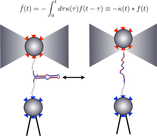
Single molecule (SM) methods give us basic insight into the mechanics of protein folding and catalysis,1−4 molecular motor translocation,5 and single nucleic acid dynamics.6 For example, SM force spectroscopy (Figure 1) monitors transitions between molecular conformational states (say the folded and unfolded state of protein) as discrete changes of force as a function of time.
Figure 1.
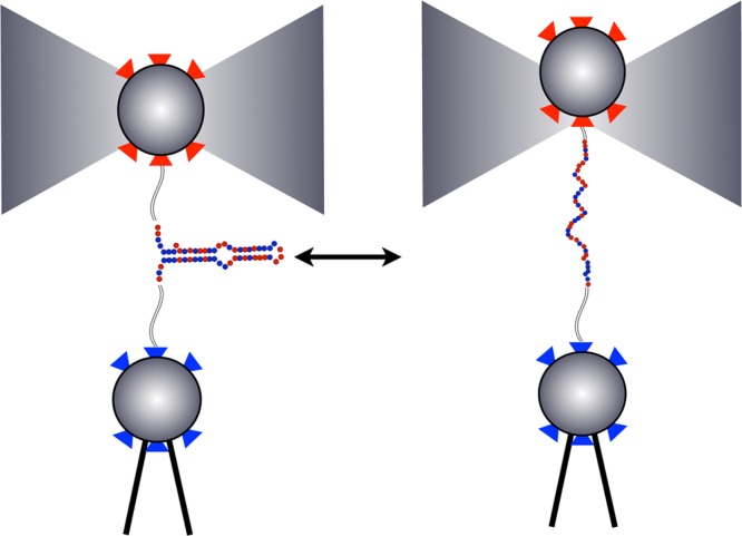
Single molecule force spectroscopy is used to monitor RNA hairpin zipping–unzipping transitions. This figure (adapted from ref (35)) shows a SM force spectroscopy setup with a single P5ab RNA hairpin33 as it undergoes transitions between a zipped and unzipped state. The bottom bead in the diagram is held fixed by a micropipet. The upper bead is held in an optical trap. In “passive mode experiments”, the optical trap is held fixed. As the hairpin transitions from the unzipped to the zipped state, it exerts force on the bead which is converted into units of piconewtons (pN) using a worm-like-chain model. See ref (35) for details.
Simple kinetic models reduce complex and noisy data into a small set of rules that govern the dynamics. The most ubiquitous of all kinetic models are simple Markov models.7−9 Two basic ingredients make up such models: (i) the topology (how states are connected to one another) and (ii) the rates describing the transition probability from state to state in units of inverse time. When data are modeled using simple Markov models, (i) and (ii) are assumed a priori and the best fit rates are generally found from data using maximum likelihood methods.10
Much of the technology used to model SM experiments was first developed to analyze data from patch clamp experiments11−16 where transitions between open (or conducting) and closed (or nonconducting) states of ion channels are monitored. Ion channels often exhibit complex kinetics. That is to say, dwell time distributions in the channels’ open and closed states can strongly deviate from single exponential behavior. To account for this nonexponential behavior, the observable states of the channel (open and closed) can be modeled as aggregates of microscopic states. In this context, a generalization of simple Markov models called aggregated Markov (AM) models17−22 is used. AM models, as applied to SM experiments, assume ahead of time how many states are in each aggregate and how all microscopic states are connected to one another, i.e., the topology, and assume that all allowed transitions between microscopic states are Markov. There are unintended consequences to these assumptions: since there are fewer observables than there are microscopic states in AM models, such models are under-determined. Even for very simple problems, an infinite number of AM models can be consistent with the data.20 Thus, relationships between some rates can be specified (or rates assumed identical) to resolve this indeterminacy.14
Furthermore, SM data is also noisy. For instance, in SM force spectroscopy, it may not always be clear whether an apparent excursion from the high force state to the low force state and then back to the high force state is due to noise or due to an actual conformational change in the single molecule. Hidden Markov (HM) models have traditionally been used in SM experiments to tackle this challenge.10 HM models start by assuming (i) a model, for example, an AM model with all of its built-in assumptions and (ii) statistics of the noise. Then, given (i) and (ii), the HM model picks transitions between states from the noisy time trace while simultaneously determining the model parameters (for the case of AM models, the parameters would be the rates of transition between states). To be clear, HM and AM models are not mutually exclusive.19 Rather, we can think of the hidden AM model as being a further generalization of an AM model. Given multiple reasonable models, Bayesian approaches have been developed to discriminate between models.23
Our goal here is to build on this body of work and lift some of its most stringent assumptions. In previous work, we presented a method for tackling noisy SM data starting from a very general non-Markov model class.36 The mathematics which are relevant to this work are presented in a self-contained way in the Appendix. Here our main focus is to apply our method to single molecule force spectroscopy data and interpret the results we obtain from our analysis.
Our method is called the non-Markov memory kernel (NMMK) method because, as we will discuss, our dynamics are governed by memory kernels which are not a priori assumed to satisfy the Markov property. Our goal is to extract the memory kernel from the data in a principled fashion from the force spectroscopy data. We will do so in a two-step process. First, we pick out transitions from the data in an objective, model-independent way24,25 and obtain noisy dwell time histograms in various states. Next, we extract from each histogram a memory kernel. The memory kernels will turn out to be our model. They contain a full description of the system dynamics—just like the topology and rates contain a full description of the dynamics for AM models. To extract the memory kernel from noisy histograms, we will adapt the method of image reconstruction.26−29 In this way, we will show how we can let the entire SM data set “speak for itself” by allowing it to select for the best model. By not assuming a predetermined model, we neither waste data nor bias our interpretation of the transitions in the raw data. A Markov model will only emerge from this analysis if it is warranted by the data; it is not assumed a priori. Furthermore, the NMMK method provides a model which is unique given the data, unlike AM models.
We will apply our method to SM force time traces obtained from P5ab, a 22 base pair RNA hairpin taken from a Tetrahymena thermophila ribozyme.33 From our analysis emerges a more textured, complex dynamics than could otherwise be obtained by forcing the data onto a simple prespecified model. In particular, the analysis suggests that not all transitions are Markov, implying the existence of an intermediate state of the RNA hairpin. The NMMK method presented here is general and could in principle be applied to data originating from a wide variety of SM methods, as well as bulk data. We will also discuss some improvements to the method we suggest and some of its limitations and compare our method to other approaches.
2. Theoretical Methods
2.1. The Generalized Master Equation
In the NMMK model, the dynamics—described by a generalized master equation—are governed by a memory kernel κ(t)
| 1 |
where f(t) denotes a dwell time distribution. This dwell time distribution can be a marginal distribution in a particular state, say A, or a conditional distribution for being in A for time t, given that the system was previously in B for some time t′. There is a memory kernel for each type of dwell time distribution. AM models are a special type of model where the kinetics are fully characterized by the set of marginal dwell time distributions for each state and the set of conditional dwell time distributions between all pairs of states.18 A renewal process is fully described by its marginal dwell time distributions.
For simplicity, we will only consider stationary processes and focus our attention on marginal dwell distributions. The mathematics of the memory kernel formulation are developed in some generality elsewhere.36 Here, we summarize important highlights relevant to the RNA hairpin.
If f(t) is a single exponential, then the memory kernel, κ(t), is a δ-function. That is, in such a state, there is no memory. This is the signature of a Markov process. However, suppose f(t) is a double exponential
| 2 |
with a1, a2 > 0. Then, the memory kernel shows mathematical structure beyond the δ-function spike at the origin. See Figures 2 and 3. This type of double exponential implies two competing time scales for decay from the given state. The resulting memory kernel is a δ-function at the origin which dips negative followed by a positive exponential rise back to zero. This behavior can be understood as follows: The memory kernel’s δ-function-like behavior at the origin says that the decay is memoryless for very short times. At later time points, the slower time scale has the net effect of introducing memory in the system by reducing the net decay rate. Mathematically, this amounts to having a negative component to the memory kernel, as is clear from Figure 3.
Figure 2.
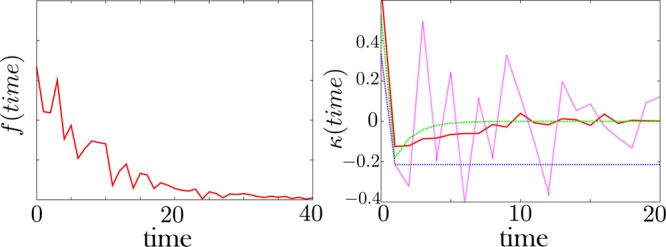
The memory kernel, κ, is extracted from the noisy dwell time histogram, f. Left: A noisy dwell time histogram generated synthetically with 30% noise. Right: The resulting memory kernel. The green curve is the exact memory kernel (0% noise). The pink curve is obtained by direct brute force inversion of the data f. The brute force inversion produces a very noisy memory kernel. For this reason, we introduce a regularization method—detailed in the Appendix—to invert a kernel from the data. The red curve is the memory kernel obtained using this method with a prior shown as a blue dotted line. The prior—also detailed in the Appendix—is our guess as to what the memory kernel should look like in the absence of data. The memory kernel and the dwell time histogram are defined by eq 1.
Figure 3.
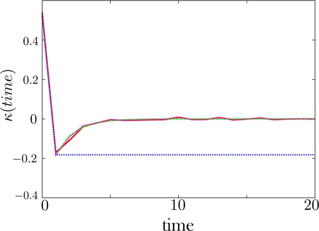
The memory kernel is reliably extracted when dwell time histograms have little associated noise. Here the noise is set to 1% in f. Our regularization scheme converges to the exact solution, as expected.
The key idea is that we need not commit ourselves to a particular mathematical form for the decay of the dwell time distribution in a state. For example, we need not be limited to exponential decays. Instead, we can ask whether the state from which we are decaying is truly a single state (i.e., single exponential decay kinetics). Otherwise, if the memory is not a sharp δ-function, we can ask: For how long does the memory in this state last? How does the memory decay in time? What does this tell us about the dynamics?
The memory kernel describing the escape from a state will depend on the time scale at which an event is being probed. That is to say, it depends on the choice of bin size for the histogram of f(t) and the sampling frequency of the original data. Large bin sizes used to build dwell histograms reduce the resolution of the model. If coarse enough bins are used in the dwell histogram, the memory kernel describing the decay curve will become Markov. On the other hand, small bins lead to noisy histograms and large associated errors around each bin resulting in memory kernels with large associated error bars themselves.
2.2. Memory Kernels Are Extracted Directly from the Data
A regularization procedure—akin to the method of image reconstruction—is used to extract the memory kernel from noisy histograms.27−30 Here we only highlight the essentials; see ref (36) and the Appendix for more mathematical details.
In discrete time, eq 1 reads
| 3 |
Our goal is to extract the memory kernel, κ, from the experimental input, f, which has an associated error for each time bin
| 4 |
where fj is the theoretical value of the dwell time histogram at time point j, while fjexp is the experimental value with coinciding error ϵj. In eq 4, we assume that error arises because trajectories are of finite length. Therefore, the counts for the dwells in bin j only approach the theoretical value if the trajectory is of infinite length. We assume that this error is not correlated from bin to bin. That is, ⟨ϵiϵj⟩ = σj2δij and ⟨ϵi⟩ = 0, where σj is the noise standard deviation.
Explicitly solving for κ from eq 3 is numerically unstable because the experimental input, f, is noisy. In the Appendix, we detail a recipe—already described in ref (36)—describing one possible regularization scheme for extracting κ from the data. This scheme has been benchmarked on synthetic data;36 see Figures 2 and 3.
2.3. Dwell Time Distributions Are Obtained by Using Change-Point Algorithms
In the previous section, we discussed how the memory kernel is extracted from noisy dwell histograms. Here, we briefly discuss how we back out those dwell histograms.
We would like the transitions in the data to be determined as objectively as possible. That is, we want transitions in the data to be determined independently of a model for the single molecule dynamics. Change-point algorithms are techniques for picking out transitions from noisy data by searching for violations of noise statistics.24,25 In this language, a positive violation of a noise statistic is indicative of a change point. Measures—such as the Schwartz information criterion (SIC)37—set the level of sensitivity to a violation of the noise statistic. In different albeit equivalent terms, the more change points are recovered, the more a model for the data is “complex”. Measures such as the SIC can therefore also be regarded as modulating the model’s complexity.
After the change-point algorithm has converged and all steps have been detected, we call the data with no noise the “de-noised time trace”. See Figure 4 for an example of a de-noised time trace. In this manuscript, we used a method which invokes the SIC called PELT (pruned exact linear time)25 to find the steps in the data because it scales favorably with data set size. Once steps are detected, it is clear from the de-noised trace that the molecule spends most of its time at very well separated discrete force levels. Usually these are a low force and a high force level. One assumption made in invoking the SIC is that the noise is uncorrelated in time. This assumption is not realized in our data; the bead corner frequency, for instance, is about 2 kHz (while the data collection frequency was 50 kHz). However, there was little difference in the change points we found by applying the SIC to the raw data versus the data where the time trace was averaged down to remove this correlation. This result was not surprising because the SIC is known to underfit data (i.e., find fewer change points than are actually present); see ref (24) for details.
Figure 4.
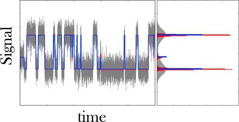
We use a change-point algorithm to find transitions in the raw SM force spectroscopy data. Left: Typical time trace obtained by SM force spectroscopy in the passive mode35 showing the transitions between a zipped and unzipped state of an RNA hairpin. The high force (i.e., high signal) state coincides with the zipped state of the hairpin. The raw data are gray, and their associated histogrammed signal intensity, also gray, shows substantial overlap between low and high force states. We apply PELT,25 a change-point algorithm, and detect the steps in the data shown in red. The histogrammed signal intensity of this de-noised time trace still shows finite breadth. K-means++ is used to cluster each dwell to its closest cluster. Here we specified three clusters, since the red histogram has three well separated peaks. The resulting quantized steps are shown in blue, and the resulting signal histogram is, by construction, an infinitely sharp peak.
As a check, we verified that all change points detected by PELT coincide with change points detected using another method, namely, an algorithm due to Kalafut.24
Next, we regroup the different force levels using a clustering algorithm (k-means++) to automate the task of identifying dwells as high or low force. The input to k-means++ is the number of clusters desired. K-means++ relies on the assumption that the traces do not substantially drift in time (i.e., that the high force state, say, remains at approximately the same value from the beginning to the end of the trace). This assumption was reasonable for our time traces. Nonetheless we also detrended our time traces as follows: (i) took the first 150 000 steps, (ii) took the lowest 10% of those values and found their median, (iii) repeated the procedure on the last 150 000 steps and took the difference between those two numbers as an estimate for the total drift, (iv) subtracted the linear drift, and (v) subsequently removed any overall offset, so that the average signal is zero.
We call the time traces to which we have applied k-means++ our “quantized time traces”. See Figure 4 for an example. We can also use k-means++ to merge well separated states (such as merge two distinct states into one) in order to verify whether the aggregated state now exhibits conformational memory. We add that both k-means++ and change-point algorithms depend on the assumptions of noise statistics, though they are free from the Markov assumption.
3. Discussion: The Unfolded (Low Force) State of RNA Shows Conformational Memory
The SM force spectroscopy data we present was collected in the passive mode, meaning the trap position is held fixed as the P5ab RNA hairpin33 transitions between zipped and unzipped states. See ref (35) for details. Multiple runs, all collected at 50 kHz over a period of 1 min, were carried out on different physical RNA fibers and at different trap positions for each fiber. Our focus here is on the majority of time traces collected where the SM is populating both high force and low force states for about equal time. Figures 5 and 6 are examples of such traces which also illustrate just how noisy data can be. Furthermore, some traces have larger noise amplitude than others and some traces show excursions to an intermediate state.
Figure 5.
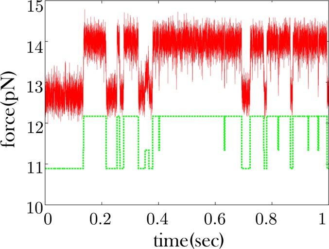
Some RNA time traces show apparent excursions to an intermediate force state. Data is shown in red. The data shown are only a fraction of the full trace which is collected over a period of 1 min. The offset green curve is the quantized time trace where three clusters were specified.
Figure 6.
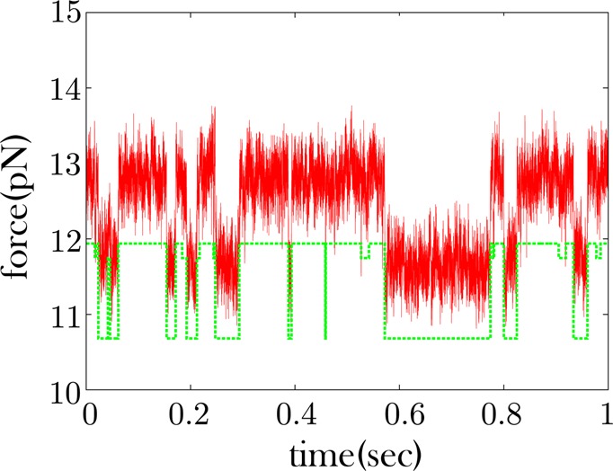
Some RNA time traces show no excursions to an intermediate force state. As with Figure 5, red is the data and green is the offset quantized time trace. This trace shows no obvious excursions to an intermediate state. These excursions could be obscured by the noise. When we cluster the force levels of the time trace into three states, we recover a state very similar in magnitude to the high force state. This implies that k-means++ is having difficulty finding the low intermediate force state it had recovered in Figure 5.
In addition, for simplicity, we only computed the memory kernel for the marginal dwell time distributions in the low and high force state. For a renewal process, these memory kernels would be a complete description of the kinetics. While we could, in principle, also compute the memory kernel for conditional dwell distributions, we have not done so here where our focus is, instead, on marginal distributions.
Figure 5 shows a longer dwell to an intermediate state at approximately 0.35 s, while Figure 6 shows very few excursions to an intermediate state, though it is possible that such excursions are obscured by the noise. We therefore would like to know if the apparent low force state of Figure 6 shows the same type of conformational memory as would be expected if we aggregate the dwells of the low and intermediate force states of Figure 5. In the passive mode, the low force state in the data coincides with the unzipped state of the RNA hairpin and the high force state coincides with the zipped state.
The main conclusions are contained in Figures 7–10. Figures 7 and 8 correspond to the memory kernels for the low and high force dwell distributions, respectively, of the fiber whose sample time trace is shown in Figure 5. Figures 9 and 10 correspond to the memory kernels for the low and high force dwell distributions, respectively, of the fiber whose sample time trace is shown in Figure 6.
Figure 7.
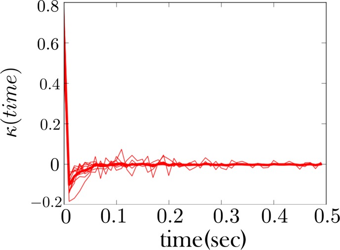
The memory kernel for the low force state (unzipped state) for an RNA hairpin shows non-Markovian behavior. We used k-means++ to cluster the low force and low intermediate force state. As expected, the memory kernel for this regrouped state shows evidence of non-Markovian behavior (or alternatively “conformational memory”), as evidenced by the negative dip in the memory kernel. A sample of a time trace of the fiber from which this memory kernel is derived is shown in Figure 5. The thicker red curve is the average memory kernel taken from the 10 lighter underlying red curves. The light red curves are collected at different trap distances.
Figure 10.
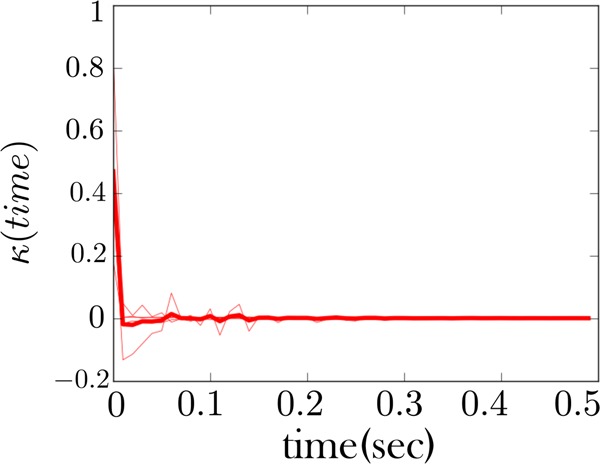
The memory kernel coinciding with the high force state (zipped state) for the fiber considered in Figure 6. This memory kernel, like Figure 8, also shows a signature of Markovianity, that is, a sharp spike at the origin.
Figure 8.
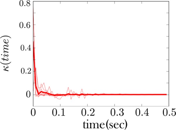
The memory kernel coinciding with the high force state (zipped state) shows Markovian behavior. This is the memory kernel for the RNA fiber considered in Figure 7. This memory kernel primarily shows a sharp spike at the origin and few features beyond this. This is a signature of Markov behavior. A sample of a time trace from the fiber from which this memory kernel is derived is also shown in Figure 5.
Figure 9.
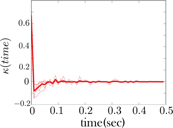
The memory kernel for the low force state of the RNA fiber whose time trace is given in Figure 6. Unlike in Figure 7, we did not regroup an intermediate and low force state here to obtain a memory kernel for the combined state. Rather, the RNA fiber in Figure 6 shows no transitions to an intermediate state. Nonetheless, the low force memory kernel shows signs of non-Markovianity consistent with Figure 7.
The fiber probed in Figure 5 shows an intermediate low force state. The same is not true of the second fiber with a sample trace shown in Figure 6 which primarily shows a high and low force state. If we use k-means++ to try to cluster the dwells at three different force magnitudes in Figure 6, we find a third state very close in magnitude to the high force state. This suggests that the change-point algorithm could not detect the intermediate force state that we had otherwise found in Figure 5.
We show in Figure 7 the memory kernel for the combined low force as well as low intermediate force states for the first fiber (whose sample trace is given in Figure 5). This memory kernel shows evidence of conformational memory, as expected since we are combining two states into one. However, other traces, like those for the second fiber (Figure 6), do not show an intermediate state being populated. Nonetheless, the memory kernel for the low force state of this fiber, Figure 9, looks qualitatively similar to that of the other fiber, Figure 7, indicating the intermediate state is present in both cases. The same is largely true of all fibers.
Furthermore, the high force state of both fibers is also qualitatively consistent, Figures 8 and 10. It primarily shows mostly Markov behavior—a strong spike at the origin and few features beyond this. This indicates that the zipped (or high force) state behaves as one state. This qualitative consistency in the memory kernel is the first of our two important theoretical conclusions drawn from these figures; see figure captions for more details.
Second, the negative dips from the memory kernel—seen in Figures 7 and 9—can be ascribed to a second time scale as we discussed earlier. However, if we interpret the negative dip as the result of a second low force state—and thus describe the low force state as an AM model—we would then be confronted with the problem of which AM model to choose from.20 That is, many AM models can be consistent with data. The latter is perhaps a counterintuitive consequence of using a discrete AM model to describe complex dynamics. Furthermore, a two-state hidden Markov approach would only find the best fit rates given the data but fail to find evidence of memory because the state structure is assumed from the onset.
Instead, here we argue that the memory kernel itself can be interpreted as a model. It indicates the duration and nature of the conformational memory.
Physically, the memory in the low force state could be attributed to two interconverting structures (a fully and partially unzipped state). Both Web servers RNAfold and AveRNA support the secondary P5ab RNA hairpin structure given in ref (33) with a bubble—a small region of non-base-pairing nucleotides as shown in Figure 1—which suggest that partial zipping is possible.
Our method is similar to some maximum-entropy-based methods which try to infer as much as possible regarding the molecular processes giving rise to the data. For instance, the method of MemExp (maximum entropy method for exponentials) extracts kinetic rate distributions from noisy histograms.30−32 To do so, MemExp posits that the dwell time distribution, f(t), is a continuous sum of exponentials31
| 5 |
and tries to extract from the noisy histogram, f(t), the rate distribution, p(k), using maximum entropy as a regularizing procedure. This inverse method of rate distribution extraction is very different from fitting the histogram to a sum of exponentials. However, since this methodology commits us to a family of exponential decays, different regularizing procedures for carrying out this inversion yield different results when the decay curves, f(t), are not exponential.32 Just as MemExp derives insight from p(k), our method derives insight from the memory kernel and the precise way in which it decays to zero. In addition, NMMK is not commited to exponential decays.
4. Conclusion
Simple kinetic models like two-state Markov models can often be helpful in drawing insight from complex data. However, not all data naturally lend themselves to such simple theoretical descriptions.39 For example, flavin reductase exhibits conformational fluctuations on multiple time scales,3 while the slow folding kinetics of phosphoglycerate kinase are indicative of kinetic traps along the folding pathway.38
With growing examples of heterogeneous kinetics in biology, there is a need for a principled strategy for drawing complex kinetic models from data. Here our strategy has been to start from a very broad class of kinetic models (anything that can be described by a memory kernel) and ask the data to pick the best model. The NMMK method is one step in developing such a principled strategy, and its advantages are as follows: (1) All the data are used in coming up with a model, the memory kernels. This is not true of fits to particular functional forms. (2) Models are not intrinsically tied to topologies, nor are they tied to exponential decay curves. (3) Models are “smooth” functions. Thus, even asking whether an additional exponential would substantially improve the fit to data makes little sense within the context of NMMK. (4) Models are unique, unlike AM models, for instance. That is, there is a one-to-one correspondence between a data set and memory kernels.
It is worth investigating whether edge detection and memory kernel extraction could be combined into a single operation, as is done with HM models. This approach would help speed up and simplify the modeling process. In addition, it would provide an elegant alternative to the binning step required when dwell durations are turned into histograms.
Acknowledgments
S.P. acknowledges the support of an IUPUI start-up and a Burroughs-Wellcome travel grant. K.D. acknowledges the support of NIH grant GM34993 and NIH/NIGMS grant R01GM09025. C.B. acknowledges NIH grant GM32543. S.M. acknowledges the NSF. S.P. thanks Craig Hetherington and Geoff Rollins for helpful discussions.
5. Appendix
Brute force inversion of fj+1exp – fj = −∑k=0j fkκj–κ to extract {κj} is numerically unstable. Image reconstruction is thus used to “regularize” the operation. Plugging eq 4 into eq 3, we have
| 6 |
where Δfj+1,jexp ≡ fj+1 – fjexp. Squaring both sides of eq 6 and taking the average with respect to the error, we find
| 7 |
We define a χ2 statistic as a sum over all time intervals
| 8 |
where N here is the number of data points in the histogram. On average, the ratio within the sum given by eq 8 is equal to 1 according to eq 7. It approaches 1 in the limit that the average given in eq 7 is taken over a large number of bins, j. If N is large enough, we can assume that χ2 ∼ N.27−30 Ideally, our goal is to select the memory kernel that makes χ2 as close to N as possible. Realistically, many values for the memory kernel can achieve such values of χ2. We thus have an under-determined problem which we resolve variationally.
We propose to maximize the objective function, F(θ, {κ}), with respect to the set {κj}
| 9 |
The regularization term is −∑j(κj + κ̅) log((κj + κ̅)/(Λj + κ̅)); {α, β} = {cos2 θ, sin θ} are Lagrange multipliers that enforce the constraints on the data; Λj is the prior on κj; and κ̅ is a constant positive parameter which ensures that the argument of the logarithm is always positive. Our estimate of the set {κj} in the absence of data is therefore κj0 = (Λj + κ̅)e–1 – κ̅. We add that our choice for the regularizing term (i.e., the entropy) in our objective function, eq 9, is used because it works for all test cases we have considered so far.
To ensure ourselves that our choice for the regularizing function yields the correct answer when we deal with real data, we benchmarked our method on fictitious data where we know what {κj} we theoretically expect; see Figures 2 and 3 and ref (36) for more examples.
There are many ways to specify our prior, Λj. We try to take advantage of the fact that, from brute force inversion, we can reliably determine the first few points of the memory kernel before error begins propagating in the determination of κj for higher j. Here we set the first two points (j = 0 and j = 1) of Λj from our brute force memory kernel as the first two points of the prior, Λj. The rest of the prior is taken to be flat.
Author Contributions
¶ J.P. and J.L. contributed equally.
The authors declare no competing financial interest.
Funding Statement
National Institutes of Health, United States
References
- Neuweiler H.; Johnson C. M.; Fersht A. R. Direct observation of ultrafast folding and denatured state dynamics in single protein molecules. Proc. Natl. Acad. Sci. U.S.A. 2010, 106, 18569–18574. [DOI] [PMC free article] [PubMed] [Google Scholar]
- Shank E. A.; Cecconi C.; Dill J. W.; Marqusee S.; Bustamante C. The folding cooperativity of a protein is controlled by its chain topology. Nature 2010, 465, 637–640. [DOI] [PMC free article] [PubMed] [Google Scholar]
- Yang H.; et al. Protein conformational dynamics probed by single-molecule electron transfer. Science 2003, 302, 262. [DOI] [PubMed] [Google Scholar]
- Yang H.; Xie X. S. Probing single-molecule dynamics photon by photon. J. Chem. Phys. 2003, 117, 10965. [Google Scholar]
- Yildiz A.; Forkey J. N.; McKinney S. A.; Ha T.; Goldman Y. E.; Selvin P. R. Myosin V walks hand-over-hand: Single fluorophore imaging with 1.5 nm localization. Science 2003, 300, 2061. [DOI] [PubMed] [Google Scholar]
- Cheng W.; Arunajadai S. G.; Moffitt J. R.; Tinoco I.; Bustamante C. Single-Base Pair Unwinding and Asynchronous RNA Release By the Hepatitis C Virus NS3 Helicase. Science 2011, 333, 1746–1749. [DOI] [PMC free article] [PubMed] [Google Scholar]
- van Kampen N. G.Stochastic Processes in Chemistry and Physics; North Holland Publishing Company: Amsterdam, The Netherlands, 1981. [Google Scholar]
- Ge H.; Pressé S.; Ghosh K.; Dill K. A. Markov processes follow from the principle of maximum caliber. J. Chem. Phys. 2012, 136, 064108. [DOI] [PMC free article] [PubMed] [Google Scholar]
- Lee J.; Pressé S.; Dill K. A. A derivation of the master equation from path entropy maximization. J. Chem. Phys. 2013, 137, 074103. [DOI] [PMC free article] [PubMed] [Google Scholar]
- McKinney S. A.; Joo C.; Ha T. Analysis of Single-Molecule FRET Trajectories Using Hidden Markov Modeling. Biophys. J. 2006, 91, 1941–1951. [DOI] [PMC free article] [PubMed] [Google Scholar]
- Hamill O. P.; Marty A.; Neher E.; Sakmann B.; Sigworth F. J. Improved patch-clamp techniques for high-resolution current recording from cells and cell-free membrane patches. Pfluegers Arch. 1981, 391, 85–100. [DOI] [PubMed] [Google Scholar]
- Hille B. Modulation of ion-channel function by G-protein-coupled receptors. Trends Neurosci. 1994, 17, 531–536. [DOI] [PubMed] [Google Scholar]
- Methfessel C.; Witzemann V.; Takahashi T.; Mishina M.; Numa S.; Sakmann B. Patch clamp measurements onXenopus laevis oocytes: currents through endogenous channels and implanted acetylcholine receptor and sodium channels. Pfluegers Arch. 1981, 407, 577–588. [DOI] [PubMed] [Google Scholar]
- Xie L.-H.; John S. A.; Ribalet B.; Weiss J. N. Phosphatidylinositol-4,5-bisphosphate (PIP2) regulation of strong inward rectifier Kir2.1 channels: multilevel positive cooperativity. J. Physiol. 2008, 586, 1833. [DOI] [PMC free article] [PubMed] [Google Scholar]
- Milescu L. S.; Akk G.; Sachs F. Maximum Likelihood Estimation of Ion Channel Kinetics from Macroscopic Currents. Biophys. J. 2005, 88, 2494. [DOI] [PMC free article] [PubMed] [Google Scholar]
- Siwy Z.; Ausloos M.; Ivanova K. Correlation studies of open and closed state fluctuations in an ion channel: Analysis of ion current through a large-conductance locust potassium channel. Phys. Rev. E 2002, 65, 031907. [DOI] [PubMed] [Google Scholar]
- Colquhoun D.; Hawkes A. G. On the Stochastic Properties of Single Ion Channels. Proc. R. Soc. London, Ser. B 1981, 211, 205–235. [DOI] [PubMed] [Google Scholar]
- Fredkin D. R.; Rice J. A. On Aggregated Markov Processes. J. Appl. Probab. 1986, 23, 208–214. [Google Scholar]
- Qin F.; Auerbach A.; Sachs F. Maximum likelihood estimation of aggregated Markov processes. Proc. R. Soc. London B 1997, 264, 375–383. [DOI] [PMC free article] [PubMed] [Google Scholar]
- Kienker P. Equivalence of Aggregated Markov Models of Ion-Channel Gating. Proc. R. Soc. London, Ser. B 1989, 236, 269–309. [DOI] [PubMed] [Google Scholar]
- Ball F. G.; Sansom M. S. P. Ion-Channel Gating Mechanisms: Model identification and Parameter Estimation from Single Channel Recordings. Proc. R. Soc. London, Ser. B 1989, 236, 385–416. [DOI] [PubMed] [Google Scholar]
- Fredkin D. R.; Montal M.; Rice J. A.. Identification of aggregated Markovian models: application to the nicotinic acetylcholine receptor. Proc. of the Berkeley Conf. in Honor of Jerzy Neyman and Jack Kiefer; Le Cam L. M., Ohlsen R. A., Eds.; Wadsworth: Belmont, CA, 1986; pp 269–289. [Google Scholar]
- Bronson J. E.; Fei J.; Hofman J. M.; Gonzalez R. L. Jr.; Wiggins C. H. Learning Rates and States from Biophysical Time Series: A Bayesian Approach to Model Selection and Single-Molecule FRET Data. Biophys. J. 2009, 97, 3196–3205. [DOI] [PMC free article] [PubMed] [Google Scholar]
- Kalafut B.; Visscher K. An objective, model-independent method for detection of non-uniform steps in noisy signals. Comput. Phys. Commun. 2008, 179, 716–723. [Google Scholar]
- Killick R., Fearnhead P., Eckley I. A.. Optimal detection of changepoints with a linear computational cost. 2011. arXiv:1101.1438v2.
- Skilling J.; Bryan R. K. Maximum entropy image reconstruction: general algorithm. Mon. Not. R. Astron. Soc. 1984, 211, 111–124. [Google Scholar]
- Bryan R. K. Maximum entropy analysis of oversampled data problems. Eur. Biophys. J. 1990, 18, 165–174. [Google Scholar]
- Gull S. F.; Daniell G. J. Image Reconstruction from incomplete and noisy data. Nature 1978, 272, 686–690. [Google Scholar]
- Skilling J.; Gull S. F. Bayesian maximum entropy image reconstruction. Lect. Notes-Mon. Series, Spatial Stat. Imaging 1991, 20, 341–367. [Google Scholar]
- Steinbach P. J.; et al. Determination of rate distributions from kinetic experiments. Biophys. J. 1992, 61, 235–245. [DOI] [PMC free article] [PubMed] [Google Scholar]
- Steinbach P. J.; Ionescu R.; Matthews C. R. Analysis of kinetics using a hybrid maximum-entropy/nonlinear-least-squares method: application to protein folding. Biophys. J. 2002, 82, 2244–2255. [DOI] [PMC free article] [PubMed] [Google Scholar]
- Voelz V. A.; Pande V. S. Calculation of rate spectra from noisy time series data. Proteins: Struct., Funct., Bioinf. 2011, 80, 342–351. [DOI] [PMC free article] [PubMed] [Google Scholar]
- Wen J.-D.; Manosas M.; Li P. T. X.; Smith S. B.; Bustamante C.; Ritort F.; Tinoco I. Force Unfolding Kinetics of RNA Using Optical Tweezers. I. Effects of Experimental Variables on Measured Results. Biophys. J. 2007, 92, 2996–3009. [DOI] [PMC free article] [PubMed] [Google Scholar]
- Elms P. J.An investigation of the mechanical properties of the molten globule state of apomyoglobin. California Institute for Quantitative Biomedical Research (QB3), University of California: Berkeley, CA, 2011. [Google Scholar]
- Pressé S.; Lee J.; Dill K. A. A memory kernel approach for extracting kinetic models from noisy data. J. Phys. Chem. B 2013, 117, 495–502. [DOI] [PMC free article] [PubMed] [Google Scholar]
- Schwartz G. Estimating the Dimension of a Model. Ann. Stat. 1978, 6, 461–464. [Google Scholar]
- Osváth S.; Sabelko J. J.; Gruebele M. Tuning the Heterogeneous Early Folding Dynamics of Phosphoglycerate Kinase. J. Mol. Biol. 2003, 333, 187–199. [DOI] [PubMed] [Google Scholar]
- Kou S. C.; Xie X. S. Generalized Langevin equation with fractional Gaussian noise: Subdiffusion within a Single Protein Molecule. Phys. Rev. Lett. 2004, 93, 180603. [DOI] [PubMed] [Google Scholar]


