Using XHMM software to detect copy number variation in whole-exome sequencing data

Abstract

Copy number variation (CNV) has emerged as an important genetic component in human diseases, which are increasingly being studied for large numbers of samples by sequencing the coding regions of the genome, i.e., exome sequencing. Nonetheless, detecting this variation from such targeted sequencing data is a difficult task of sorting out signal from noise, for which we have recently developed a set of statistical and computational tools called XHMM. In this paper, we give detailed instructions on how to run XHMM and how to use the resulting CNV calls in biological analyses.

Introduction

Numerous recent studies have implicated copy number variation (CNV) in many cancers (Pollack et al. 2002; Shlien and Malkin 2010) and severe neuropsychiatric conditions including autism (Pinto et al. 2010), schizophrenia (International Schizophrenia Consortium 2008; Stefansson et al. 2008), intellectual disability (Cooper et al. 2011), bipolar disorder, and epilepsy. The latter neuropsychiatric phenotypes are generally enriched for rare structural deletions and duplications, often from de novo germline mutations. Given the strong evidence for the role in disease of copy number variation, particularly variants that impact genes, and the large number of ongoing exome sequencing studies of disease, it is critical that researchers have extensive tools at their disposal for detecting CNV as easily and robustly as possible. Numerous methods are available for detection of CNVs from untargeted, whole-genome sequence data; these methods typically utilize multiple sources of information, from unusual mapping of read mate-pairs, from (“split”) reads that span breakpoints, and from sequencing coverage. In contrast, since exome sequencing targets non-contiguous segments of the genome, the only information readily and generally applicable is depth of coverage (Figure 1), which is still the noisiest of these data. Moreover, due to the additional targeting step (hybridization capture array), the signal-to-noise ratio in exome depth is far lower than in whole-genome experiments and, perhaps more importantly, severe biases can be introduced that obscure the relationship between raw depth of coverage and ploidy.

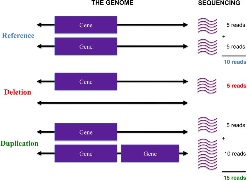
Figure 1. How genomic copy number affects depth of sequencing.

Depicted are a reference individual with two copies of a gene, an individual with only a single copy (deletion of gene on one chromosome), and an individual with an extra copy of a gene in their genome (duplication). In an idealized setting where each individual's genome is targeted at an average of 10× coverage, 5 of those reads will come from the maternal chromosome and 5 from the paternal. If one of those chromosomes is missing that gene (deletion), then only 5 reads for that gene will be observed; on the other hand, if an individual has a duplication of that gene, then a total of 15 reads will be found. In reality, noise and biases in the data make it difficult to easily and directly read off genomic copy number from such coverage information. The purpose of XHMM is to automate a procedure for performing such inference in a robust manner.

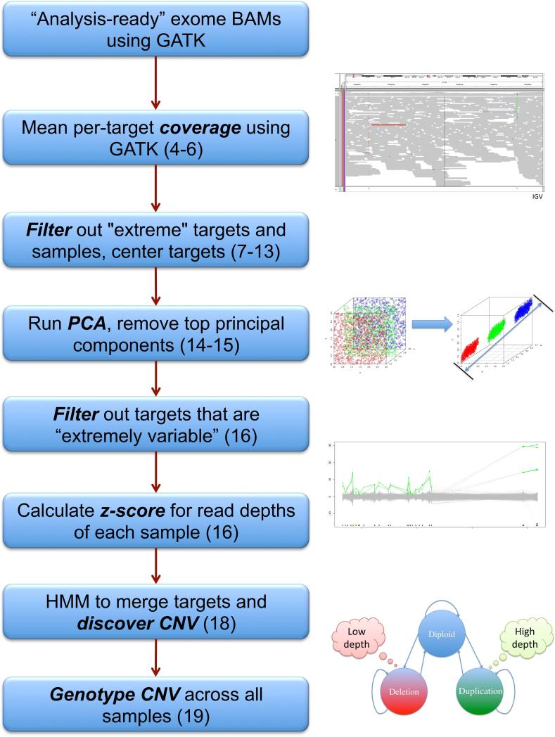
The XHMM (eXome-Hidden Markov Model) software was designed to recover information on CNVs from targeted exome sequence data (Fromer et al. 2012) and allows researchers to more comprehensively understand the association between genetic copy number and disease. The key steps in running XHMM are running depth of coverage calculations, data normalization, CNV calling, and statistical genotyping (Figure 2). The calling and genotyping stages provide extensive quality metrics that are geared toward a range of analyses that require varying degrees of filtering of putative signal from noise. This paper provides detailed instructions for running XHMM and gives examples and instructions for analyses that are possible using the CNV calls and results from XHMM.

Figure 2. Flowchart of calling CNV from exome sequence data using XHMM.

Each step in the CNV discovery and genotyping XHMM pipeline is listed, with corresponding step numbers from Basic Protocol 1 listed in parentheses. Key steps are depicted graphically on the right.

A web-based tutorial that follows a similar format to this paper is available here: http://atgu.mgh.harvard.edu/xhmm/tutorial.shtml A video tutorial is available here: http://www.broadinstitute.org/videos/broade-xhmm-discovery-and-genotyping-copy-number-variation-exome-read-depth

BASIC PROTOCOL 1: SOFTWARE INSTALLATION, DEPTH OF COVERAGE CALCULATION, FILTERING AND NORMALIZATION, CNV CALLING

The objective of this protocol is to set up the XHMM software, use it to calculate exome-sequencing depth-of-coverage information (using GATK, see below), filter the coverage data (e.g., based on GC content of exons calculated using GATK and/or based on the sequence complexity of the exons calculated using Plink/Seq, see below), normalize the coverage, and then use the normalized values to discover and statistically genotype copy number variation on an entire sample of individuals.

Necessary Resources

Installed versions of the LAPACK(http://www.netlib.org/lapack/) and pthread (https://computing.llnl.gov/tutorials/pthreads/) C libraries, which are properly accessible to the C++ compiler (e.g., in the proper path environment variables). For LAPACK to work, you may need to also install atlas and acml as well on some systems. LAPACK is used for efficiently performing the singular value decomposition (SVD) step of the principal component analysis (PCA) used for normalization of the data. Pthread is for speeding up certain computations using multiple parallel processing threads (currently still not highly developed in XHMM, as we have found the steps following the read depth calculations to be quite fast in practice, even for datasets of thousands of samples; see Commentary).

Installed copy of the Genome Analysis ToolKit (GATK). See: http://www.broadinstitute.org/gatk/download We will assume that you have installed GATK in ‘Sting/dist/GenomeAnalysisTK.jar’.

For certain optional (but preferred steps), it's also necessary to install the latest version of Plink/Seq (http://atgu.mgh.harvard.edu/plinkseq). Up-to-date code can be downloaded here: https://bitbucket.org/statgen/plinkseq/get/master.zip

The human reference sequence database file (seqdb) can be downloaded here: http://atgu.mgh.harvard.edu/plinkseq/resources.shtml

The following user-input files are required in a number of the following steps and so are listed here once for convenience:

1. Reference genome FASTA file and associated BWA index file (http://biobwa.sourceforge.net/bwa.shtml). In the examples here, we refer to this file as human_g1k_v37.fasta (which can be downloaded as part of the GATK resource bundle: http://gatkforums.broadinstitute.org/discussion/1213/what-s-in-the-resource-bundle-and-how-can-i-get-it).

2. List of exome targets, in the ‘interval_list’ GATK format (http://gatkforums.broadinstitute.org/discussion/1204/what-input-files-does-thegatk-accept). We refer to this file as EXOME.interval_list. This file should contain non-overlapping, sorted intervals. As an example, two lines for chromosome 22 coding sequence exons are:

   • 22:16449425-16449804
   • 22:17071768-17071966

Downloading Software and Installation

The latest version of the XHMM software can be found in the BitBucket repository, with a compressed zip file found at: https://bitbucket.org/statgen/xhmm/get/master.zip Then run the following commands from the command line:

1. Unzip the zipped source files: unzip master.zip

2. Change to the source directory: cd statgen-xhmm-*

3. Run make to install the software (which starts by automatically compiling the included hmm++ library): make

Run GATK DepthOfCoverage to get sequencing depths

To calculate the depth of sequencing coverage, you need to start with the exome sequencing reads in BAM format. You should use “analysis-ready” BAM files and associated index files, as generated by the BWA/Picard/GATK pipeline described here for next-generation sequencing data processing: http://www.broadinstitute.org/gatk/guide/best-practices

A key part of this pipeline includes the marking of PCR duplicates, so that they are not included in depth of coverage statistics. While variations of this pipeline, and even other pipelines to produce the BAM files for XHMM input, have been successfully employed by various users, this is not currently supported here.

For the calculation of coverage, users should take advantage of their computational resources (such as computing clusters) by calculating the depth of coverage in parallel for various subsets of the samples. In the example here, we assume the user has split the list of individuals into two groups, though in practice you should split the sample in a way that best takes advantage of your machines.

4.Splitup the list of locations for the per-sample BAM files into two files:

group1.READS.bam.list

group2.READS.bam.list

Throughout the subsequent steps in this protocol, the names of the output files were chosen to use the generic ‘DATA’ identifier, though this can be changed to use a more project-specific naming scheme.

5. Run GATK for depth of coverage (once for samples in group1 and once for group2):

java -Xmx3072m -jar Sting/dist/GenomeAnalysisTK.jar

-T DepthOfCoverage -I group1.READS.bam.list -L EXOME.interval_list

-R human_g1k_v37.fasta

-dt BY_SAMPLE -dcov 5000 -l INFO --omitDepthOutputAtEachBase –omitLocusTable

--minBaseQuality 0 --minMappingQuality 20

--start 1 --stop 5000 --nBins 200

--includeRefNSites

--countType COUNT_FRAGMENTS

-o group1.DATA

java -Xmx3072m -jar Sting/dist/GenomeAnalysisTK.jar

-T DepthOfCoverage -I group2.READS.bam.list -L EXOME.interval_list

-R human_g1k_v37.fasta

-dt BY_SAMPLE -dcov 5000 -l INFO --omitDepthOutputAtEachBase –omitLocusTable

--minBaseQuality 0 --minMappingQuality 20

--start 1 --stop 5000 --nBins 200

--includeRefNSites

--countType COUNT_FRAGMENTS

-o group2.DATA

The key parameters here are ‘-dt BY_SAMPLE -dcov 5000’, which limits the depth to 5,000 reads for each individual sample; ‘--minBaseQuality 0’, which allows bases of any quality be included in the count; ‘--minMappingQuality 20’, which stringently requires that reads be mapped to the reference genome with sufficient certainty (e.g., uniqueness) to be counted in the depth statistics; and ‘--countType COUNT_FRAGMENTS’, which instructs GATK to properly count any overlapping parts of paired-end mate pairs only once.

Combine GATK Depth of Coverage outputs

6. Run the following command to extract the mean coverage for each exon interval for each sample and merge them all into a single sample-by-target matrix (samples are in the rows, targets are in the columns):

xhmm --mergeGATKdepths -o DATA.RD.txt

--GATKdepths group1.DATA.sample_interval_summary

--GATKdepths group2.DATA.sample_interval_summary

Optional: run GATK to calculate GC content of targets

These two optional steps calculate per-target GC content and creates a list of targets with extreme GC content that you can use to perform upfront filtering of exome targets expected to pose more challenges to detecting CNV due to their more extreme properties (e.g., high and low GC content targets tend to be captured less well on exome hybridization arrays).

7. Calculate the GC content of each coding exon (exome target) using GATK:

java -Xmx3072m -jar Sting/dist/GenomeAnalysisTK.jar

-T GCContentByInterval -L EXOME.interval_list

-R human_g1k_v37.fasta

-o DATA.locus_GC.txt

8. Create a list of all exome targets to be excluded, based on their GC content: cat DATA.locus_GC.txt | awk ‘{if ($2 < 0.1 || $2 > 0.9) print $1}’ > extreme_gc_targets.txt

In this case, we are choosing to exclude all exons with more than 90% or less than 10% GC content in the human reference sequence. If, for example, you would like to call CNV on all targets, these values can be changed to be more liberal (or skip this step entirely).

Optional: run Plink/Seq to calculate sequence complexity of targets

These four optional steps calculate the fraction of repeat-masked bases (Smit and Hubley 2008) in each target and creates a list of targets with low complexity for you to filter out upfront.

9. Convert exome target list to Plink/Seq format:

statgen-xhmm-*/sources/scripts/interval_list_to_pseq_reg

EXOME.interval_list > EXOME.targets.reg

10. Load exome target list into a Plink/Seq exome database file: pseq . loc-load

--locdb EXOME.targets.LOCDB --file EXOME.targets.reg --group targets

11. Run Plink/Seq to calculate the per-target repeat-masking fraction (download the seqdb file along with the Plink/Seq code, as described above):

pseq . loc-stats --locdb EXOME.targets.LOCDB --group targets --seqdb seqdb | awk ‘{if (NR > 1) print $_}’ |

sort -k1 -g | awk ‘{print $10}’ | paste EXOME.interval_list - |

awk ‘{print $1“t”$2}’

> DATA.locus_complexity.txt

12. Create a list of all exome targets to be excluded, based on the fraction of repeat-masked sequence (as calculated by RepeatMasker (Smit and Hubley 2008)): cat DATA.locus_complexity.txt | awk ‘{if ($2 > 0.25) print $1}’ > low_complexity_targets.txt

As for the GC content target filter, you can change the threshold here to be more permissive (lowering the value of 0.25) if you prefer to attempt to call CNV on a larger portion of the exome. Or, you can skip this filtering step altogether if you wish.

Filter samples and targets and prepare for normalization

The next step is to remove any samples and targets with outlier read depth values (including those determined in previous steps or those chosen by the particular parameters in this command), and then mean-center the targets in preparation for the PCA-based normalization in the next step.

13. Use the xhmm ‘matrix’ command to process the read-depth matrix: xhmm --matrix -r DATA.RD.txt --centerData --centerType target

-o DATA.filtered_centered.RD.txt

--outputExcludedTargets DATA.filtered_centered.RD.txt.filtered_targets.txt

--outputExcludedSamples DATA.filtered_centered.RD.txt.filtered_samples.txt

--excludeTargets extreme_gc_targets.txt --excludeTargets low_complexity_targets.txt

--minTargetSize 10 --maxTargetSize 10000

--minMeanTargetRD 10 --maxMeanTargetRD 500

--minMeanSampleRD 25 --maxMeanSampleRD 200

--maxSdSampleRD 150

If you chose above to not filter the targets based on GC content or repeat-masking, then you should leave off the corresponding command-line parameters here (‘--excludeTargets extreme_gc_targets.txt’ and ‘--excludeTargets low_complexity_targets.txt’, respectively).

The semantics of the other parameters here are to record the excluded targets and samples (to be used in later steps), exclude targets with extreme GC content or low complexity, exclude targets of less than 10 bp or more than 10 kbp, exclude targets with a mean depth over all samples less than 10 reads or more than 500 reads, exclude samples with a mean depth over all targets less than 25 reads or more than 200 reads or with extremely high variance (greater than 150), and lastly to center each column of the matrix so that the mean target value is 0 (‘--centerData --centerType target’). Importantly, if you expect your experimental setup to result in mean depths that deviate from these generic values, then you need to change these values to reflect your dataset and only remove true outlier targets and samples. The distributions of these values are plotted in the R scripts accompanying XHMM (see Basic Protocol 2).

Run principal component analysis (PCA) on mean-centered data

14. Run PCA to determine the strongest independent ways (principal components) in which the data varies:

xhmm --PCA -r DATA.filtered_centered.RD.txt --PCAfiles DATA.RD_PCA

This outputs 3 files to be used in the next step:

1. DATA.RD_PCA.PC.txt: the data projected into the principal components

2. DATA.RD_PCA.PC_LOADINGS.txt: the loadings of the samples on the principal components

3. DATA.RD_PCA.PC_SD.txt: the variance of the input read depth data in each of the principal components

Normalize mean-centered data using PCA information

Once we have determined how the read depth data varies, we would like to remove the strongest signals that are driven by factors that do not reflect true CNV (Figure 3).

Figure 3. Normalization by removal of top principal components.

In this “toy” example (of 4 samples targeted at 10 exons), the 4×10 read depth matrix is first decomposed into the principal components (the key axes in which the read depth varies), the variance of the data in each such component, and the sample loadings (the coefficients of each sample in each component). Then, in this example, it is estimated (not shown) that the two largest principal components correspond to non-CNV read depth effects, based on their large relative contribution to the variance of the read depth data. These components are thus removed by zeroing them out, and the reconstructed read depth matrix will be used for CNV calling.

15. Remove the top principal components and reconstruct a normalized read depth matrix:

xhmm --normalize -r DATA.filtered_centered.RD.txt --PCAfiles DATA.RD_PCA

--normalizeOutput DATA.PCA_normalized.txt

--PCnormalizeMethod PVE_mean --PVE_mean_factor 0.7

The number of principal components to be removed is determined by the ‘--PCnormalizeMethod PVE_mean --PVE_mean_factor 0.7’ argument, which indicates that XHMM will remove any principal component in which the data variance is greater than 0.7 times the mean variance over all components. This argument can be changed to retain additional components or remove more components for normalization, if you decide that XHMM is not optimally normalizing the data (see Basic Protocol 2 for data visualization). Or, the ‘PCnormalizeMethod’ can be changed to ‘numPCtoRemove’ along with using the ‘--numPCtoRemove' to explicitly specify how many components you want to remove.

Filter and calculate z-scores for the data

16. Now that we have PCA-normalized the depth data, we still need to remove any targets that have very high variance that may be reflective of failed normalization (Figure 9). Note, however, that even after this filtering step, exon targets with very high variance in the original read depths still remain with relatively high (though attenuated) variance in depth after normalization (see Figure 10), since large differences between samples and targets are by necessity maintained in order to preserve existing CNV signal as well. Then, for each sample, we use XHMM to calculate z-scores of read depths by centering relative to all target depths in that sample:

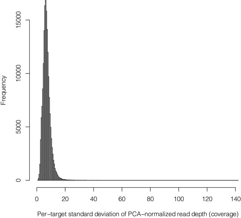
Figure 9. Distribution of post-normalization target variance.

Before XHMM calculates z-scores and the HMM is run to call CNV for each sample (CNV “discovery”), we perform a final filtering step. Specifically, we remove any targets that have “very scattered” read depth distributions post normalization. These can be thought of as targets for which the normalization may have failed, and it is better to remove such strong effects (still likely to be artifacts) to prevent them from drowning out other more subtle signals. In detail, we removed any targets with large standard deviations of their post-normalization read depths across all samples. As a (proto-typical) example, we see here that the small fraction of targets with standard deviations any larger than the 30 to 50 range were removed (in this case, for a scenario of ~100× mean sequencing coverage).

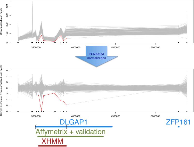
Figure 10. XHMM copy number variation region plot.

This plot shows each sample's original and normalized read depths at each of the targets in focus, which are connected by gray lines. If the sample has a called deletion, then it is colored in red, and duplications in green. Gene names are added below to annotate the genomic region, and black dots and bars mark the location of the exome targets. In this example from the XHMM paper (Fromer et al. 2012), also shown are the overlaps between the XHMM call (marked in red), the Affymetrix chip-based call and custom validated region (Kirov et al. 2012), and the exome-targeted region of DLGAP1 (delineated by square brackets). By following Basic Protocol 2, a regional plot is produced for each CNV called in each individual (as found in the .xcnv file): plot_CNV/sample_*.png. Alternatively, a PDF with all stages of read depth adjustment (from unnormalized [top panel here] to final normalized values used for CNV calling [bottom panel here]) can be generated by passing the PLOT_ONLY_PNG=FALSE argument to the XHMM_plots() function in the example_make_XHMM_plots.R script file.

xhmm --matrix -r DATA.PCA_normalized.txt

--centerData --centerType sample --zScoreData

-o DATA.PCA_normalized.filtered.sample_zscores.RD.txt

--outputExcludedTargets

DATA.PCA_normalized.filtered.sample_zscores.RD.txt.filtered_targets.txt --outputExcludedSamples

DATA.PCA_normalized.filtered.sample_zscores.RD.txt.filtered_samples.txt --maxSdTargetRD 30

Here again, we record any targets filtered out (for use in the next step), specifically, those targets with a post-normalized standard deviation greater than 30. This value is intended to remove outlier targets, but you will need to tailor this value based on inspection of the distribution of these values in your data (see Basic Protocol 2 for data visualization).

The ‘--centerData --centerType sample --zScoreData’ parameters instruct XHMM to calculate the z-score of the per-sample read depth vector rd as: z(rd) = [rd – mean(rd)] / standard deviation(rd)

Filter original read-depth data to restrict to same samples and targets as filtered, normalized data

17. Next, we take the pre-normalized read depths and remove the same targets and samples that we removed during the normalization process. This matrix will be used for annotation purposes in the subsequent CNV “discovery” and “genotyping” steps:

xhmm --matrix -r DATA.RD.txt

--excludeTargets DATA.filtered_centered.RD.txt.filtered_targets.txt

--excludeTargets

DATA.PCA_normalized.filtered.sample_zscores.RD.txt.filtered_targets.txt

--excludeSamples DATA.filtered_centered.RD.txt.filtered_samples.txt

--excludeSamples

DATA.PCA_normalized.filtered.sample_zscores.RD.txt.filtered_samples.txt -o DATA.same_filtered.RD.txt

Call CNVs in normalized data (“Discovery”)

Now that we have normalized the read depth values for your exome data, you are ready to actually make CNV calls in each sample. To do this, we use a hidden Markov model (HMM) with certain properties that were derived from a large-scale trio data set (Fromer et al. 2012). These parameters, which determine the rate and length of the CNV called, are specified in the XHMM model parameters file; default values are provided in the params.txt file distributed with the XHMM source code. The 9 values in this file correspond to quantities that respectively define the:

1. Exome-wide CNV rate

2. Mean number of targets in a CNV call

3. Mean distance between targets within a CNV (in KB)

4. Mean of DELETION z-score distribution

5. Standard deviation of DELETION z-score distribution

6. Mean of DIPLOID z-score distribution

7. Standard deviation of DIPLOID z-score distribution

8. Mean of DUPLICATION z-score distribution

9. Standard deviation of DUPLICATION z-score distribution

These parameters are used in the HMM for CNV “discovery” and “genotyping” (next steps), and you may need to modify them to suit the needs of your particular project. For example, to increase the number of CNV calls, increase the first parameter from its default value of 1e-8, e.g., to 1e-7. However, as we have found these parameters to be highly sensitive to known CNV in a number of scenarios, it is often the case that there will still be an abundance of CNV calls output at this stage, many of which will need to be filtered out using the quality metrics associated with each CNV call (see, e.g., Basic Protocol 3).

18. Run the HMM Viterbi algorithm to call CNV in each sample:

xhmm --discover -p params.txt

-r DATA.PCA_normalized.filtered.sample_zscores.RD.txt

-R DATA.same_filtered.RD.txt

-c DATA.xcnv -a DATA.aux_xcnv -s DATA

The main output file is DATA.xcnv, which contains one line for each CNV called in an individual. The columns in this file denote the following quantities for that CNV, which are defined as in our previous paper (Fromer et al. 2012):

The main output file is DATA.xcnv, which contains one line for each CNV called in an individual. The columns in this file denote the following quantities for that CNV, which are defined as in our previous paper (Fromer et al. 2012):

SAMPLE	sample name in which CNV was called
CNV	type of copy number variation (DEL or DUP)
INTERVAL	genomic range of the called CNV
KB	length in kilobases of called CNV
CHR	chromosome name on which CNV falls
MID_BP	the midpoint of the CNV (to have one genomic number for plotting a single point, if desired)
TARGETS	the range of the target indices over which the CNV is called (NOTE: considering only the FINAL set of post-filtering targets)
NUM_TARG	# of exome targets of the CNV
Q_EXACT	Phred-scaled quality of the exact CNV event along the entire interval - Identical to EQ in .vcf output from genotyping
Q_SOME	Phred-scaled quality of some CNV event in the interval - Identical to SQ in .vcf output from genotyping
Q_NON_DIPLOID	Phred-scaled quality of not being diploid, i.e., DEL or DUP event in the interval - Identical to NDQ in .vcf output from genotyping
Q_START	Phred-scaled quality of “left” breakpoint of CNV - Identical to LQ in .vcf output from genotyping
Q_STOP	Phred-scaled quality of ‘right” breakpoint of CNV - Identical to RQ in .vcf output from genotyping
MEAN_RD	Mean normalized read depth (z-score) over interval - Identical to RD in .vcf output from genotyping
MEAN_ORIG_RD	Mean read depth (# of reads) over interval - Identical to ORD in .vcf output from genotyping

Statistically assess discovered CNVs in all samples (“Genotyping”)

As is the case for SNP and insertion/deletion (indel) calling from next-generation sequencing data (DePristo et al. 2011), it is beneficial to collect all variation called across multiple samples and then uniformly re-genotype these variants in each sample. To do this, we calculate the quality metrics defined above for each sample (even if the CNV was not originally called in that sample) and apply certain rules (Fromer et al. 2012) for establishing the genotype of a particular sample.

19. Run the HMM forward-backward algorithm to quantitatively genotype each called CNV in all samples:

xhmm --genotype -p params.txt

-r DATA.PCA_normalized.filtered.sample_zscores.RD.txt

-R DATA.same_filtered.RD.txt

-g DATA.xcnv -F human_g1k_v37.fasta

-v DATA.vcf

The VCF file that is output contains ‘haploid’ genotypes for each individual, or a missing genotype if the normalized read depth is not definitive. The rationale behind the ‘haploid’ genotypes represents the best-guess allele call for that sample across the entirety of the corresponding genomic region (diploid, deletion, or duplication). Since XHMM currently does not differentiate between heterozygous and homozygous deletions, or between a copy number of 3 or higher, only a single prediction value is made for each sample. In addition to the actual genotypes, the VCF file also contains a range of quality metrics, which you can use to compare a particular CNV between different samples, e.g., see Basic Protocol 3 for calling de novo CNV. As the VCF file output itself contains the explicit definitions of each of these metrics, these will not be detailed here, except to mention that the EQ (corresponding to the probability of the exact CNV event across a genomic region) is the main value used to define the ‘hard’ genotype calls provided in that file.

An important point to note here is that, as is standard practice with VCF files, each row (corresponding to a genomic region originally called as CNV in some sample) is genotyped independently of all other rows. Thus, if one sample has a particularly long CNV that encompasses a smaller CNV called in a different sample, then the first sample will likely be genotyped as having both of these CNV (on their corresponding rows in the VCF), whereas the second sample will likely not have the first CNV genotyped as variant since for that sample the larger region encompasses both diploid and CNV sequence, resulting in a missing genotype call (denoted by ‘.’ in the VCF file).

BASIC PROTOCOL 2: VISUALIZE RESULTING CNV USING R SCRIPTS

After having run Basic Protocol 1 for installation of XHMM, depth of coverage calculation, data filtering, normalization, discovery of CNV, and statistical genotyping, the R scripts accompanying the main XHMM C++ code allow you to visualize each of the stages in the XHMM pipeline. We now describe the data visualization protocol.

Necessary Resources

For visualization, we use the R statistical analysis software, which can be downloaded here: http://www.r-project.org

Also, install the latest version of Plink/Seq (http://atgu.mgh.harvard.edu/plinkseq). Up-to-date code can be downloaded here: https://bitbucket.org/statgen/plinkseq/get/master.zip

1. Run Plink/Seq to obtain an annotated list of which genes overlap each exome target: pseq . loc-intersect

--group refseq --locdb locdb

--file EXOME.interval_list

--out annotated_targets.refseq

The RefSeq human transcript and gene database file (locdb) can be downloaded here: http://atgu.mgh.harvard.edu/plinkseq/resources.shtml

Or, follow the instructions there for generating a custom transcript/gene locdb database.

2. Edit the file statgen-xhmm-*/sources/scripts/example_make_XHMM_plots.R and update the following variables:

1. XHMM_PATH should point to the path of the root statgen-xhmm-* directory.

2. PLOT_PATH should point to the path of the desired location for output plots.

3. JOB_PREFICES should point to the prefix of files chosen in Basic Protocol 1 (if you chose to change it from the generic ‘DATA’ used in the commands given above).

4. JOB_TARGETS_TO_GENES should point to the Plink/Seq exon annotation file from step 1 (named ‘annotated_targets.refseq.loci’).

5. Optional: If you have sample traits that could be useful in understanding which principal components correspond to such sample properties, then either PEDIGREE_FILE or PHENOTYPES_FILE (but not both) should point to the corresponding files in Plink/Seq ‘pedinfo’ or ‘phenotype’ formats. See http://atgu.mgh.harvard.edu/plinkseq/input.shtml#ped and http://atgu.mgh.harvard.edu/plinkseq/input.shtml#phe, respectively, for more details.

3. Run the master R script for data visualization (note this may take a number of hours to run, depending on the number of samples and CNV calls):

Rscript example_make_XHMM_plots.R

4. Inspect the output plots. The key files are described in the corresponding figure legends.

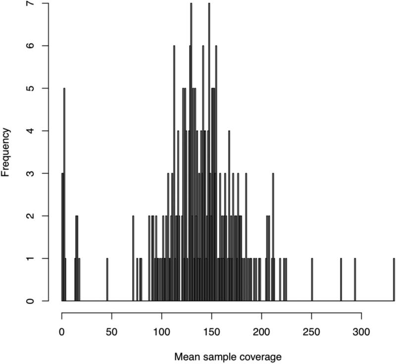
1. mean_sample_coverage.pdf (Figure 4)

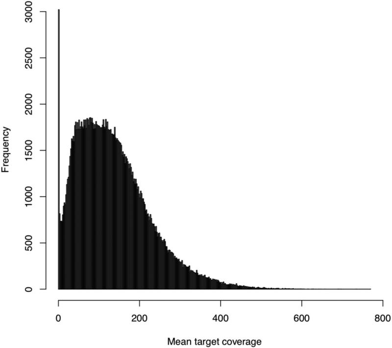
2. mean_target_coverage.pdf (Figure 5)

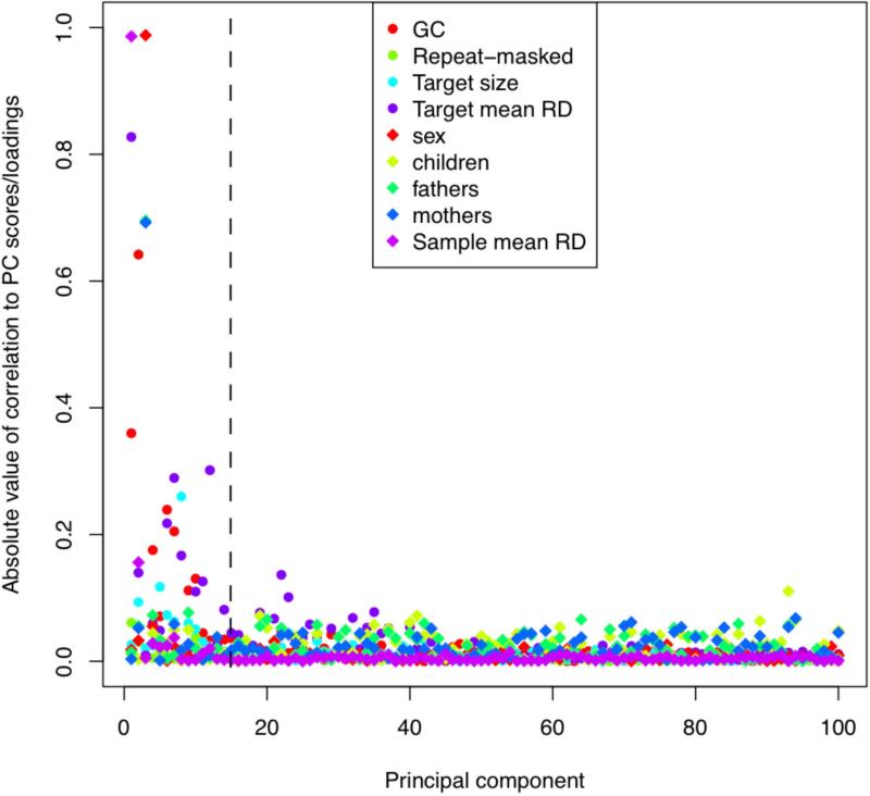
3. PC_correlations.pdf (Figure 6)

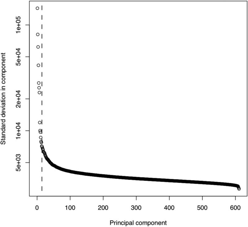
4. PC_stddev.pdf (Figure 7)

5. PC/PC.*.png (Figure 8)

6. per_target_sd.pdf (Figure 9)

7. plot_CNV/sample_*.png (Figure 10)

Figure 4. Sample coverage plot.

This shows the sample-wide distribution of exome-wide sequencing coverage, where each per-sample coverage value is the mean of the coverage values calculated for each exome target (which itself is the mean coverage at all of its bases in that particular sample). In this experiment, we sequenced each sample to a mean coverage of 150×, so that we expect a typical sample to indeed have 150 reads covering an average base in an average exome target.

Figure 5. Exome target coverage plot.

Analgous to Figure 4, this plot gives the target-wide distribution of coverage (over all samples). That is, each per-target coverage value is the mean of the per-sample coverage values at that target (where again, this is the mean coverage at all of its bases in that sample). As above, since our goal was to have 150× coverage exome-wide, we'd expect each target to have around 150× coverage, but we see here that there is high variability in target coverage. For example, some targets have as much 400× coverage (averaged over all samples), and we also see a non-trivial number of targets that have 0 coverage for all samples (e.g., targets where capture has presumably failed).

Figure 6. Principal component analysis (PCA) normalization.

This plot compares each of the principal components (PC) to known sample and target features (samples features can be added in step 2E of Basic Protocol 2). The dotted line (at PC = 15) indicates that XHMM automatically removed the first 15 components based on their significant relative variance. In this plot, we consider known sample and target features (that XHMM did not incorporate in its decision to remove them). We see that these first 15 PC tend to show correlation with various target features (colored circles) such as GC content and the mean depth of sequencing coverage at that target, and also with various sample features (colored diamonds) such as gender and mean depth of sequencing for that sample. On the other hand, there is a marked change in quality of the PC after the first 15 or so, with a sudden drop-off in the levels of correlation with genome-wide and batch effects expected to strongly bias the read depth of coverage.

Figure 7. “Scree” plot for the PCA.

This plot shows the standard deviation of the depth data independently ascribed to each of the principal components. This case is typical, where we see that the cut-off automatically detected by XHMM corresponds to a significant drop in the variance (an “elbow” in the curve). Note the log scale of the y axis.

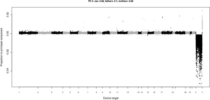
Figure 8. Read depth projected in a principal component.

This principal component (the 3^rd one, in this instance) has found the variance in read depth due to gender differences, with males having lower coverage on the X chromosome and higher coverage on the Y. Therefore, the loadings for this component have a correlation of 0.99 with the gender of the samples. Note that the R script creates the ‘PC’ sub-directory, which contains plots of the read depth data projected into each of the principal components: PC/PC.*.png.

BASIC PROTOCOL 3: CALL DE NOVO CNV USING PLINK/SEQ

For most analyses, it is incumbent upon the researcher to consider the metrics and properties of the data set as a whole before considering any one particular CNV call. That is, here we typically recommend filtering on both the SQ quality threshold (the “Q_SOME” column in the .xcnv file) and filtering on sample-wide frequency to obtain a high-quality call set.

As a specific example, we focus here on the details of calling de novo CNV (CNV arising as new mutations in a child and not present in the child's parents) from the statistically genotyped call set output by XHMM, as this nicely demonstrates these principles. Note that this protocol typically requires on the order of 25 to 50 trios (father, mother, and child) with exome sequencing in order to successfully estimate population frequencies in subsequent filtering steps.

The basic principle in calling de novo CNV (or any de novo variant) is that selecting for variants present in a child but not in the parents will highly enrich for artifactual calls in the child and instances where CNV may have gone undetected in the parents. Since both artifacts and CNV in the parents are more likely to occur at regions of apparently “common” CNV (due to truly being common in the population or to a recurring sequencing artifact), we start by filtering on estimated population frequency to remove both common CNV and frequent noise from being called as a de novo CNV. To do this, we utilize the Plink software for frequency filtering of the CNV

(http://pngu.mgh.harvard.edu/~purcell/plink/cnv.shtml) in the VCF file after having run XHMM in Basic Protocol 1.

Necessary Resources

Plink software (download from http://pngu.mgh.harvard.edu/~purcell/plink/download.shtml).

Filter CNV based on frequency estimated from the sample

1. Follow Support Protocol 1 to obtain Plink-formatted CNV files of the XHMM calls output in Basic Protocol 1.

Now, we will find any CNV that overlaps 50% of another CNV that occurs in more than 10% of all samples (a relatively liberal frequency threshold to remove only common CNV and artifacts).

2. Calculate the number of samples in the data:

set NUM_SAMPLES = ‘cat DATA.fam | wc -l’

3. Set the frequency threshold at 10% of the total number of samples:

set THRESH_NUM = ‘echo “0.1 * $NUM_SAMPLES” | bc | awk ’{x = $1; if (x != int(x)) {x = int(x)+1} print x}’’

Note that the syntax in the commands in steps 2 and 3 may need to be modified slightly if using a UNIX shell other than ‘csh’ or ‘tcsh’ (e.g., ‘bash’ or ‘sh’).

4. plink --cfile DATA --cnv-freq-exclude-above $THRESH_NUM --cnv-overlap 0.5 --cnv-write --out DATA.maf_0.1

5. cat DATA.maf_0.1.cnv | awk ’{if (NR>1) print $3“:“$4”-”$5}’ | sort | uniq > DATA.maf_0.1.CNV_regions.txt

6. Now, we exclude all such common regions from the VCF file:

cat DATA.vcf |

awk ‘{if (substr($1,1,1)==“#”) {print $_}

else {found=-1; cmd = “grep -w “$3” DATA.maf_0.1.CNV_regions.txt”;

cmd | getline found; close(cmd);

if (found != -1) {print $_}}}’

> DATA.maf_0.1.vcf

Detect putative de novo CNV by strict use of XHMM quality scores

7. Create a new Plink/Seq project that will contain the XHMM-called variants: pseq DATA new-project

8. Load a Plink/Seq pedinfo file (http://atgu.mgh.harvard.edu/plinkseq/input.shtml#ped) containing the child-parent pedigree relationships (named ‘DATA.pedinfo’ here): pseq DATA load-pedigree --file DATA.pedinfo

9. Load the frequency-filtered VCF file into the Plink/Seq project:

pseq DATA load-vcf --vcf DATA.maf_0.1.vcf

10. Now, assuming you've chosen a quality score filter of 60 to call de novo CNV on the autosomes, run:

pseq DATA cnv-denovo --mask reg.ex=chrX,chrY --minSQ 60 --minNQ 60 --out DATA which outputs a file called DATA.denovo.cnv. This lists CNV that are likely to be transmitted from parent to child, likely to be non-transmitted, and those likely to be de novo CNV in the children. Each of these sets results from requiring sufficient certainty of having a CNV or not in each of the parents and the child, respectively. For example, for de novo CNV, this requires that the SQ is greater than 60 for the child (high probability that there is some CNV) and that NQ in each of the parents is above 60 (high probability of no CNV in either parent). See our previous paper for how a quality score threshold (e.g., 60) can be titrated based on such transmission data, i.e., by choosing the minimum such threshold for which the expected rate of 50% transmission from parent to child is empirically achieved (Fromer et al. 2012).

BASIC PROTOCOL 4: COMPARE XHMM CNV TO EXTERNAL CNV CALL SET

Sometimes it is beneficial to compare the CNV called by XHMM to those called by a different algorithm on the same exome-sequencing data, or using an entirely different technology applied to the same samples. As an example, consider the case where we would like to estimate the sensitivity of XHMM to detecting the larger CNV called from Affymetrix array data for the same samples.

1. Follow Support Protocol 1 to obtain Plink-formatted CNV files of the XHMM calls.

2. Test the sensitivity of the XHMM CNV in DATA.cnv toward the Affymetrix CNV in AFFY.cnv:

statgen-xhmm-*/sources/scripts/perl/compare_CNVs.pl

AFFY.cnv DATA.cnv DATA.fam EXOME.interval_list

> xhmm_VS_affy.txt

3. Inspect the output file xhmm_VS_affy.txt. The file contains one row for each of the Affymetrix CNV and asks how many exome targets are overlapped by the CNV (i.e., to understand potential callability) and how far the closest XHMM-called CNV is from the Affymetrix CNV, and how many and which exome targets are in that XHMM CNV (if any). The output header includes detailed descriptions of the output columns, but the key ones are:

A. SAMPLE: Sample ID of the Affymetrix CNV.

B. DIST: Distance between closest XHMM CNV(s) and the Affymetrix CNV in SAMPLE. This is equal to 0 only if there is an XHMM CNV call that overlaps the Affymetrix CNV.

C. CLOSEST_TARGET_DIST: Distance between the closest exome target(s) and the Affymetrix CNV. This is equal to 0 only if the exome sequencing has a target that overlaps the Affymetrix CNV.

For example, the sensitivity of XHMM to the Affymetrix calls is defined as the total number of Affymetrix CNV overlapped by an XHMM call, divided by the total number of Affymetrix CNV theoretically detectable by exome sequencing. In other words, the number of (non-header) output rows with a DIST value of 0, divided by the total number of output rows with a CLOSEST_TARGET_DIST value of 0 (or a DIST value of 0, for the unlikely case where the XHMM CNV may partially overlap the Affymetrix CNV even though it does not overlap any exome targets).

SUPPORT PROTOCOL 1: CONVERT XHMM CNV CALLS TO PLINK FORMAT

The Plink software contains many desired functionalities for handling, filtering, and analyzing CNV (http://pngu.mgh.harvard.edu/~purcell/plink/cnv.shtml), including case-control association. It is thus desirable to convert to Plink format for certain analyses:

1. Create a Plink-format .fam file

(http://pngu.mgh.harvard.edu/~purcell/plink/data.shtml#ped) listing all samples analyzed: grep “^#CHROM” DATA.vcf | awk ‘{for (i = 10; i <= NF; i++) print $i,1,0,0,1,1}’ > DATA.fam

2. Convert the XHMM .xcnv call set to Plink .cnv format:

statgen-xhmm-*/sources/scripts/xcnv_to_cnv DATA.xcnv > DATA.cnv

3. Create a Plink .map file:

plink --cfile DATA --cnv-make-map --out DATA

SUPPORT PROTOCOL 2: REQUEST SUPPORT FROM THE XHMM USERS FORUM

1. Visit the XHMM users Google Group to ask a question or browse previous posts: https://groups.google.com/a/broadinstitute.org/group/xhmm-users/

2. Or, send an email directly to:

xhmm-users@broadinstitute.org

COMMENTARY

Background Information

The XHMM software and protocols detailed in this paper represent one of the state-ofthe-art packages for discovering and genotyping copy number variants (CNV) from targeted exome sequencing data. The past decade has seen an abundance of evidence indicating the critical role that CNVs play in cancer susceptibility, gene expression, metastasis, and treatment options, as well as a large role in neuropsychiatric and developmental diseases. Since many recent disease studies have chosen a targeted exome sequencing approach, it is critical that researchers have clear instructions on how to utilize tools such as XHMM that were developed to detect coding-region CNVs in order to maximize the associations with disease that are detectable from sequence data. XHMM has recently been used in large-scale studies of disease, including schizophrenia (Fromer et al. 2012) and autism (Poultney et al. 2013; Lim et al. 2013).

A number of related software packages do exist, but a number of these require specific assumptions about the data, such as analyses of tumors vs. normal tissues (Sathirapongsasuti et al. 2011) or require explicit modeling of potential biases (Wu et al. 2012). On the other hand, the data-driven normalization performed by CoNIFER (Krumm et al. 2012) is most similar to that performed here, though we found the subsequent CNV calling step in XHMM to be more robustly supported by the statistical framework of hidden Markov models and its derived quality scores (Fromer et al. 2012); detailed definitions of these scores are given in step 18 of Basic Protocol 1.

In the future, we plan to enhance the XHMM and related software packages. Some possible additions include the use of sequencing-based SNP calls and sub-exon sequencing information to improve the reliability of CNV calls and their breakpoints. We will also add additional Plink/Seq modules to leverage the XHMM-produced VCF file to detect copy number events whose breakpoints fall within (and disrupt) a gene (Fromer et al. 2012), which have been hypothesized to have the potential to be particularly deleterious.

Critical Parameters

Key user-tunable parameters for Basic Protocol 1 (calling CNV) include:

1. GATK depth-of-coverage parameters (minBaseQuality and minMappingQuality), which determine which reads and bases are counted in the per-exon depth calculations (Step 5).

2. Sample and target filters based on mean coverage (minMeanTargetRD, maxMeanTargetRD, minMeanSampleRD, maxMeanSampleRD, maxSdSampleRD), which exclude outlier samples and targets before running PCA (Step 13).

3. Parameter to determine the number of principal components removed during normalization (PVE_mean_factor, which is a fraction between 0 and 1, and specifies that XHMM will remove any principal component in which the data variance is greater than PVE_mean_factor times the mean variance over all components (Step 15).

4. Target filter based on high variance among samples (maxSdTargetRD) that remains after PCA-based normalization (Step 16).

5. The 9 HMM parameters in the params.txt file that determine the rate, size, number of exons, and required read depth deviations of CNV to be called (Step 18).

For Basic Protocol 3 (calling de novo CNV), the key parameters include:

1. Frequency filter for consideration of rare CNV (value of 0.1 in Step 3).

2. XHMM quality score threshold (minSQ and minNQ), which determine how certain the data corresponds to having a CNV call and to a non-CNV call (i.e., diploid state), respectively (Step 10).

Troubleshooting

If a user encounters problems or bugs in running the XHMM software, the user should follow Support Protocol 2. The XHMM user forum allows the user to browse previous questions that may depict similar issues encountered by other users, or the user can post a question to be answered by the XHMM authors or other users.

Time Considerations

While run times for XHMM will vary depending on computational resources, exome size, etc., the total run time of Basic Protocol 1 is generally a function of the number of samples. As an example, when running on 100 samples, we have found that calculating depth of coverage exome-wide (for Agilent SureSelect Human All Exon v.2) took 5-6 hours when running each sample separately (i.e., 100 groups in step 4 below). After that, running all subsequent XHMM commands on all 100 samples on a single processor required only 1-2 hours in total. At no point did any process require more than 3-4 GB of memory to run.

Literature Cited

- Cooper Gregory M., Coe Bradley P., Girirajan Santhosh, Rosenfeld Jill A., Vu Tiffany H., Baker Carl, Williams Charles, et al. A Copy Number Variation Morbidity Map of Developmental Delay. Nature Genetics. 2011 Sep;43(9):838–846. doi: 10.1038/ng.909. doi:10.1038/ng.909. [DOI] [PMC free article] [PubMed] [Google Scholar]
- DePristo Mark A., Banks Eric, Poplin Ryan, Garimella Kiran V., Maguire Jared R., Hartl Christopher, Philippakis Anthony A., et al. A Framework for Variation Discovery and Genotyping Using Next-generation DNA Sequencing Data. Nature Genetics. 2011 May;43(5):491–498. doi: 10.1038/ng.806. doi:10.1038/ng.806. [DOI] [PMC free article] [PubMed] [Google Scholar]
- Fromer Menachem, Moran Jennifer L., Chambert Kimberly, Banks Eric, Bergen Sarah E., Ruderfer Douglas M., Handsaker Robert E., et al. Discovery and Statistical Genotyping of Copy-Number Variation from Whole-Exome Sequencing Depth. The American Journal of Human Genetics. 2012 Oct 5;91(4):597–607. doi: 10.1016/j.ajhg.2012.08.005. doi:10.1016/j.ajhg.2012.08.005. [DOI] [PMC free article] [PubMed] [Google Scholar]
- International Schizophrenia Consortium Rare Chromosomal Deletions and Duplications Increase Risk of Schizophrenia. Nature. 2008 Sep 11;455(7210):237–241. doi: 10.1038/nature07239. doi:10.1038/nature07239. [DOI] [PMC free article] [PubMed] [Google Scholar]
- Kirov G, Pocklington AJ, Holmans P, Ivanov D, Ikeda M, Ruderfer D, Moran J, et al. De Novo CNV Analysis Implicates Specific Abnormalities of Postsynaptic Signalling Complexes in the Pathogenesis of Schizophrenia. Molecular Psychiatry. 2012 Feb;17(2):142–153. doi: 10.1038/mp.2011.154. doi:10.1038/mp.2011.154. [DOI] [PMC free article] [PubMed] [Google Scholar]
- Krumm Niklas, Sudmant Peter H., Ko Arthur, O'Roak Brian J., Malig Maika, Coe Bradley P., Quinlan Aaron R., Nickerson Deborah A., Eichler Evan E. Copy Number Variation Detection and Genotyping from Exome Sequence Data. Genome Research. 2012 Aug 1;22(8):1525–1532. doi: 10.1101/gr.138115.112. doi:10.1101/gr.138115.112. [DOI] [PMC free article] [PubMed] [Google Scholar]
- Lim Elaine T., Raychaudhuri Soumya, Sanders Stephan J., Stevens Christine, Sabo Aniko, MacArthur Daniel G., Neale Benjamin M., et al. Rare Complete Knockouts in Humans: Population Distribution and Significant Role in Autism Spectrum Disorders. Neuron. 2013 Jan 23;77(2):235–242. doi: 10.1016/j.neuron.2012.12.029. doi:10.1016/j.neuron.2012.12.029. [DOI] [PMC free article] [PubMed] [Google Scholar]
- Pinto Dalila, Pagnamenta Alistair T., Klei Lambertus, Anney Richard, Merico Daniele, Regan Regina, Conroy Judith, et al. Functional Impact of Global Rare Copy Number Variation in Autism Spectrum Disorders. Nature. 2010 Jul 15;466(7304):368–372. doi: 10.1038/nature09146. doi:10.1038/nature09146. [DOI] [PMC free article] [PubMed] [Google Scholar]
- Pollack Jonathan R., Sørlie Therese, Perou Charles M., Rees Christian A., Jeffrey Stefanie S., Lonning Per E., Tibshirani Robert, Botstein David, Børresen-Dale Anne-Lise, Brown Patrick O. Microarray Analysis Reveals a Major Direct Role of DNA Copy Number Alteration in the Transcriptional Program of Human Breast Tumors. Proceedings of the National Academy of Sciences. 2002 Oct 1;99(20):12963–12968. doi: 10.1073/pnas.162471999. doi:10.1073/pnas.162471999. [DOI] [PMC free article] [PubMed] [Google Scholar]
- Poultney Christopher S., Goldberg Arthur P., Drapeau Elodie, Kou Yan, Harony-Nicolas Hala, Kajiwara Yuji, De Rubeis Silvia, et al. Identification of Small Exonic CNV from Whole-Exome Sequence Data and Application to Autism Spectrum Disorder. The American Journal of Human Genetics. 2013 Oct 3;93(4):607–619. doi: 10.1016/j.ajhg.2013.09.001. doi:10.1016/j.ajhg.2013.09.001. [DOI] [PMC free article] [PubMed] [Google Scholar]
- Sathirapongsasuti Jarupon Fah, Lee Hane, Horst Basil A. J., Brunner Georg, Cochran Alistair J., Binder Scott, Quackenbush John, Nelson Stanley F. Exome Sequencing-based Copy-number Variation and Loss of Heterozygosity Detection: ExomeCNV. Bioinformatics. 2011 Oct 1;27(19):2648–2654. doi: 10.1093/bioinformatics/btr462. doi:10.1093/bioinformatics/btr462. [DOI] [PMC free article] [PubMed] [Google Scholar]
- Shlien Adam, Malkin David. Copy Number Variations and Cancer Susceptibility. Current Opinion in Oncology. 2010 Jan;22(1):55–63. doi: 10.1097/CCO.0b013e328333dca4. doi:10.1097/CCO.0b013e328333dca4. [DOI] [PubMed] [Google Scholar]
- Smit AFA, Hubley R. RepeatModeler Open-1.0. 20082008–2010 [Google Scholar]
- Stefansson Hreinn, Rujescu Dan, Cichon Sven, Pietiläinen Olli P. H., Ingason Andres, Steinberg Stacy, Fossdal Ragnheidur, et al. Large Recurrent Microdeletions Associated with Schizophrenia. Nature. 2008 Sep 11;455(7210):232–236. doi: 10.1038/nature07229. doi:10.1038/nature07229. [DOI] [PMC free article] [PubMed] [Google Scholar]
- Wu Jiantao, Grzeda Krzysztof R., Stewart Chip, Grubert Fabian, Urban Alexander E., Snyder Michael P., Marth Gabor T. Copy Number Variation Detection from 1000 Genomes Project Exon Capture Sequencing Data. BMC Bioinformatics. 2012 Nov 17;13(1):305. doi: 10.1186/1471-2105-13-305. doi:10.1186/1471-2105-13-305. [DOI] [PMC free article] [PubMed] [Google Scholar]