

Abstract
Previous work describes a computational solvation model called semi-explicit assembly (SEA). The SEA water model computes the free energies of solvation of nonpolar and polar solutes in water with good efficiency and accuracy. However, SEA gives systematic errors in the solvation free energies of ions and charged solutes. Here, we describe field-SEA, an improved treatment that gives accurate solvation free energies of charged solutes, including monatomic and polyatomic ions and model dipeptides, as well as nonpolar and polar molecules. Field-SEA is computationally inexpensive for a given solute because explicit-solvent model simulations are relegated to a precomputation step and because it represents solvating waters in terms of a solute’s free-energy field. In essence, field-SEA approximates the physics of explicit-model simulations within a computationally efficient framework. A key finding is that an atom’s solvation shell inherits characteristics of a neighboring atom, especially strongly charged neighbors. Field-SEA may be useful where there is a need for solvation free-energy computations that are faster than explicit-solvent simulations and more accurate than traditional implicit-solvent simulations for a wide range of solutes.
1. Introduction
There is a need for computer methods that can calculate the aqueous solvation free energies of solute molecules accurately and efficiently.1−13 Two common approaches are explicit-solvent and implicit-solvent models. Explicit-solvent models14,15 provide a physically accurate and atomistically detailed model of solvent, but they can be computationally expensive. Implicit-solvent models, such as Poisson–Boltzmann (PB),11,12 generalized Born (GB),7,16 and weighted surface area (WSA) approaches,17−21 are computationally efficient because they treat water as a continuum. However, they are sometimes inaccurate, smearing out the particulate nature of water molecules,22−24 and they may have limited transferability to situations for which they have not been optimized.20,21
Solvation modeling has often been improved by combining the advantages of implicit- and explicit-solvent models.25−36 One such approach is the semi-explicit assembly (SEA) water model.37,38 In the SEA approach, water’s solvation behavior is precomputed in explicit-solvent simulations of water around model spheres that are then combined together as building blocks to represent any given solute structure at run time. The solvation free energy ΔGsolv for a target solute molecule is calculated from a sum over solvating waters. SEA has been shown to predict efficiently the air-to-water transfer free energies (ΔGhyd) of small-molecule solutes in both prospective and retrospective studies13,38 with reasonable accuracy. Even so, the SEA model does not give accurate solvation free energies of ions or solutes having high charge density.
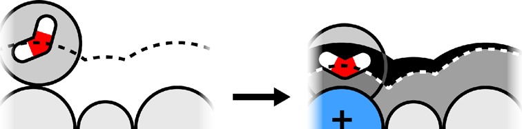
Here, we describe field-SEA, a considerable improvement over SEA, which gives accurate free energies of transfer of ions and charged solutes, at no additional computational cost and with no degradation of the predictions for nonpolar and uncharged polar solutes. In overview, we studied full MD simulations of ionic and neutral solutes in TIP3P water, described below, and found that the results could be captured by using a solvation free-energy field surface (in field-SEA), instead of using precomputed waters (as in SEA). The free-energy field is fast to compute. Moreover, we found that a weakly charged solute atom that is adjacent to a strongly charged solute atom retains some of the restrictions of its solvating water molecules that its neighboring charge has; see Figure 1. Field-SEA captures this effect using an adaptive boundary method.
Figure 1.
A solvent–water molecule around a solute molecule. On the left, each solute atom (weakly charged) has a predefined radius, irrespective of its neighboring solute atoms, leading to the locus of water centers shown by the black dashed curve. On the right, one solute atom is strongly charged, leading to two consequences: its own solvating water molecule is pulled in tightly, and neighboring solute atoms have tighter water interactions too. We refer to the latter effect as an adaptive boundary. The energetic consequences can be large. Such effects may not be captured in simplified solvation models that treat atoms as having fixed radii, independent of neighboring atoms.
2. Theory and Methods
Below, we describe the field-SEA approach to computing solvation free energies. The original SEA model is described elsewhere,37,38 and our related explicit-solvent and linearized Poisson–Boltzmann equation modeling39 (LPBE) are described in the Supporting Information (SI).
2.1. Precalculations of Charged Spheres in Explicit Water
In both the original SEA37 and the new field-SEA described here, the calculation of solvation free energies is divided into two steps. First, in a precomputation step, various model spheres are solvated in an explicit-solvent model, such as TIP3P. This provides a database of component free energies that are used in the second step. In the second step, at the run time, any given solute molecule of interest is assembled from an appropriate concatenation of these spheres. The solute’s solvation free energy is computed by summing the component sphere free energies. On the one hand, this approach provides the speed advantages of simple additivity-based models as we only need to perform the first step once for a given solvent model. On the other hand, this procedure is more accurate than additivity-based approaches because (1) SEA sums are regional, not local, and (2) the database encodes the microscopic response observed in explicit-solvent simulations. The original SEA captures the water solvation shell as discrete waters. The new field-SEA instead captures the solvation free energy using a continuous solvation field.
To do this, the charging free energies for a series of Lennard-Jones (LJ) spheres solvated in TIP3P water were calculated with thermodynamics integration (TI) in the set of precomputations (see Explicit Solvent Free Energy Calculations in the SI). We construct a free-energy contour (see SI Figure S1) as a combination of the electric field at the first solvation shell boundary (E = Q/rw2, where E is the signed magnitude of the electric field, Q is the sphere’s charge, and rw is the distance from the sphere center to the first peak of the water oxygen’s radial distribution function, RDF, around the given sphere), the curvature C = 1/rw at this boundary, and the charging free energy of the spheres. Within each charge step (ΔQ), all of the data of free energy, electric field, and curvature were fitted to a formula, which can be taken as an expansion of the Born model
| 1 |
Equation 1 will be used to calculate the free energy associated with any surface spot on an arbitrary solute–solvent boundary (Esub). This free energy could also be calculated from interpolation between data points on the free-energy contour.
In addition to a charging free-energy contour, we also need a contour for estimating the explicit-solvent-accessible surface of a given solute molecule. To generate this, we calculated the RDF of water oxygen around each charged sphere and picked the first peak in the RDF, denoted as the boundary-sphere distance rw. All of the rw values from these spheres and their charge and LJ parameters (σLJ and εLJ) were used to build an rw contour.
2.2. Construction of Solute Dot Surfaces
To generate a solvent-accessible surface for a given solute, an rw for each atom is first calculated from interpolation with its partial charge, σLJ, and εLJ on the rw contour. A Lee–Richards surface40 is then constructed from the nonoverlapping sections of these rw spheres centered on their associated atom sites. We call this surface the fixed rw boundary.
The fixed rw boundary is dependent upon only the individual parameters of the surface atoms. For solute molecules with multiple partial charge sites (especially molecular ions, where strong electric fields are involved), a more physical representation of the explicit-solvent-accessible surface would be one that responds to the whole solute’s electric field. In other words, the surface–atom distance, rw, is determined not only by the surface atom’s partial charge, but also by neighboring atoms’ charges. Taking into account such collective electrostatic effects, we adjust the fixed rw boundary in an adaptive manner, described by the following three-step procedure:
(1)We cull all surface segments within 1.4 Å of any solute atom. As we are starting with a Lee–Richards solvent-accessible surface, the minimum rw possible in the surface construction is half of a water molecule diameter (corresponding to a solute atom with a 0 Å radius). This partial-culling process simply removes potential numerical instabilities from surface sites overlapping solute atom centers while providing some adjustable starting surface sites that penetrate within the fixed rw boundary.
(2) We adjust rw adaptively. We calculate the electric field at a given dot a about atom A
| 2 |
where N is the number of solute atoms, ria represents a vector from atom i to surface dot a, and ria is its length; signa = 1 when rAa·∑i=1N (qi/ria)ria ≥ 0, and signa = −1 when rAa·∑i=1N (qi/ria)ria < 0, and rAa is the vector from atom A to dot a. From the electric field, we calculate the corresponding charge by
| 3 |
where rAa is the length of vector rAa. We interpolate with this new charge and atom A’s LJ parameters to get a new rw, rw,new. In addition, we assume that rw cannot expand (if rw,new > rw,original, we let rw,new = rw,original). This nonexpansion assumption is supported by solute–solvent boundary plots of model diatomic solutes (see SI Figure S2). Finally, the rw,new’s of all atom’s potential surface dots are averaged to yield an rw for this atom, used in the later culling process.
(3) We cull the buried dots adaptively. Because each dot–atom distance (e.g., daA) is adjusted independently in the above procedure, the shell of potential surface dots about an atom will no longer be spherical. Thus, culling buried dots is no longer a simple process of eliminating dots within a neighboring atom’s rw, and an adaptive culling process is needed. To adaptively cull “buried” surface dots, when we check whether a given dot a is buried by a neighboring atom B, we first determine a corresponding charge at dot a from the electric field at this dot. This is used along with atom B’s LJ parameters to get a new rw, rw,Badp, following the above rw adjustment procedure. We compare the dot–atom distance, daB, with rw,Badp, to determine if the dot is buried in atom B. If daB is less than rw,Badp, it is removed from the set of potential surface dots.
We call the new dot surface resulting from the above culling procedure the adaptive boundary. Our term field-SEA refers both to the field and to the adaptive boundary. The adaptive nature of the boundary only pertains to multiatom solutes; the adaptive and fixed rw boundaries are identical for single-atom solutes, like monatomic ions. While our adaptation procedure could, in principle, be applied iteratively, we found no further improvement after a single calculation.
2.3. Calculation of Solvation Free Energies by Summing Surface Components
The charging free energy can be calculated for any given field-SEA surface via
| 4 |
where Ndot is the total number of surface-exposed dots, mI is the total number of dots (exposed + occluded) for corresponding atom I (each surface dot, j, of atom I, only corresponds to 1/mI of this atom sphere’s total surface area or total solvation free energy), and Esub,j is the subenergy associated with exposed surface dot j, calculated from the free-energy contour. Here, Esub,j is calculated from eq 1 using the signed magnitude of the electric field, Ej, and the curvature at dot j, 1/rIj. Ej is defined as negative when Ej·rIj < 0, where Ej is the electric field (vector) at dot j, rIj is the vector from atom I to its surface dot j, and rIj is this vector’s length. Now, we take the total solvation free energy to be the sum of polar and nonpolar components37
| 5 |
Assuming the polar component of the free energy of transfer (ΔGpol) can be uniquely described by both the surface electric field and geometry of the solute, this molecular ΔGpol can be accurately calculated from the simple summation of the surface dots’ energies process described above. We consider the ΔGsolv of monatomic ions as an initial test. For molecular solutes, to account for the role of solute conformation in the solvation free energy, we average ΔGsolv results from calculations on 50 conformations (though 10 conformations are usually enough; see the SI). These solute conformations were generated from 5 ns TIP3P water MD simulations with a 100 ps snapshot interval.38
3. Results and Discussion
3.1. Solvation of Monatomic Ions
We developed field-SEA because of the errors that we observed in simpler methods in solvating ions; see Figure 2. The explicit-solvent curve shows the hydration asymmetry discussed by others,22,41,42 where positively charged solutes are less favored than negatively charged solutes of similar size. LPBE results do not directly capture this hydration asymmetry without altering the solute–solvent boundary43,44 (note the symmetry of the curve). The original SEA does capture the asymmetry but not with high accuracy.
Figure 2.
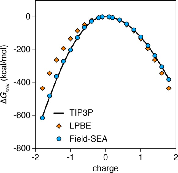
ΔGsolv as the function of a model LJ sphere (σ = 0.22 nm, ε = 0.06538 kJ/mol) charge for TIP3P, LPBE, and field-SEA. For comparison at infinite-dilution conditions, an Ewald correction is applied to the TIP3P and field-SEA results.
Here, we tested field-SEA on the solvation free energies of monatomic ions using ion parameters developed by Aqvist45 or Joung and Cheatham46 (Table S2, SI). These ions have different sizes and charges; therefore, they have different charge densities. Table 1 and Figure S3 (SI) show the results of field-SEA calculations, compared with LPBE and TIP3P. LPBE results using the LJ surface do not capture quantitatively the ΔGsolv of ions with high charge densities. In contrast, field-SEA reproduces the TIP3P ΔGsolv values regardless of the specific LJ parameters and charges. These results indicate that field-SEA is accurately reproducing explicit-solvent free energies of solvation of monatomic ions, provided that their charge and LJ parameters are near or encompassed within the range of the rw and free-energy contours.
Table 1. Errors, MSE/RMSE (kcal/mol), in ΔGsolv versus TIP3P Results for Different Solute Sets from LPBE and Field-SEA Using a Fixed-Sphere Boundary versus an Adaptive Boundary.
| solute seta | LPBE | field-SEA (fixed rw) | field-SEA |
|---|---|---|---|
| ±1 atomic ions (13) | –0.8/18.9 | –0.5/2.9 | –0.5/2.9 |
| Aqvist Mg2+, Ca2+ | >200 | 2.3/3.9 | 2.3/3.9 |
| diatomic solutes (22) | 15.5/33.7 | 10.9/26.1 | –0.2/6.9 |
| neutral solutes (504) | –1.35/1.64 | 0.38/1.23 | 0.01/0.82 |
| molecular ions (35) | 0.5/8.3 | 10.9/11.7 | 1.6/4.8 |
| dipeptides (22) | –0.3/4.6 | 4.2/5.0 | 1.1/2.6 |
Numbers in parentheses are the number of solutes.
3.2. Adaptive Boundary Importance in Molecular Solvation
A common approximation in simplified solvation models is to suppose that atoms have fixed “atom types”, where any particular solute atom has a given value of charge and radius, independent of its atomic neighbors. However, our TIP3P explicit-solvent simulations described below show that this approximation is a source of error. How the solvation surface is constructed can introduce errors into the free energies of a solvation model.47−50 Our explicit-solvent simulations show that the solvation shell is not just a simple union of the spherical surfaces of all of the atoms making up the solute molecule. Imagine a diatomic solute with partially charged atom A covalently connected to partially charged atom B. Our TIP3P simulations show that when atom A attracts water molecules, it also shrinks the solvation shell of waters around atom B. In this way, the solvation surface around the diatomic molecule A–B can be more complex than the simple union of independent spherical solvation shells around atoms A and B. To address such situations, we developed an adaptive method that gives a more explicit-like solvation boundary.
To test our adaptive boundary method, we made up 22 fictitious diatomic solutes (see SI Table S4), computed their solvation free energies, and compared to their solvation in TIP3P. We constructed these solutes by taking pairs of ordinary simulation atom types, placing them at fixed covalent bond distance apart, and giving each atom a charge and radius that we could vary systematically over the series. Because of the fictitious charges that we give them, these are not molecules observed in nature. However, they are physically plausible molecules that provide us with a systematic series for learning about how explicit-solvent models handle solvated charges.
Figure 3 shows the computed free energies of these diatomic solutes from field-SEA when using the fixed rw and adaptive boundaries in comparison to explicit-solvent TIP3P simulations. LPBE and original SEA results are shown in the SI instead of here for the sake of simplicity. In summary, we find that when the TIP3P ΔGsolv is weak, for example, when the charge density of solute atoms is low, the fixed rw boundary works fairly well. When the ΔGsolv grows to −100 kcal/mol and larger (more negative), it becomes increasingly important to use an adaptive boundary. These strongly solvated model molecules often have large, unbalanced partial charges on the solute atoms, and these situations lead to exaggerated distortions of the explicit solvation shell.
Figure 3.

Field-SEA ΔGsolv for model diatomic solutes (triangles: Fixed rw; circles: adaptive boundary) compared to TIP3P simulations. The line indicates the idealization of zero error.
Figure 4 shows how a neighboring solute atom can affect the solvation shell about another atom. The fixed rw and adaptive boundaries are identical in Figure 3A as both carbon atoms are weakly charged and there is only minor collective electrostatic perturbation on the boundary. However, when the solutes are more highly charged and large charging energies are involved, as in Figure 3B, the weakly charged carbon atom’s solvation shell will be distorted by its neighboring highly charged oxygen atom. In this case, water molecules penetrate more deeply into the carbon’s solvent-accessible surface to better solvate the oxygen charge (the right part of the white curve in the dark blue region). Also, water molecules pack more tightly around the carbon atom and reduce its apparent rw (the left part of the white curve in the blue and light blue regions). Both of these effects are captured well by adaptive field-SEA boundaries, leading to field-SEA charging energies that are in excellent agreement with explicit simulation results.
Figure 4.
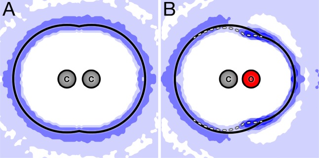
Maps of the water–oxygen density around (A) weakly charged and (B) strongly charged diatomic solutes. The blue contours indicate water density greater than the bulk value, with the darker blue regions indicating the enhanced water probability density. The black line shows the nonadaptive fixed rw boundary. For the weakly charged diatomic, the adaptive and nonadaptive boundaries coincide. The white line shows the adaptive boundary. For the charged diatomic, the adaptive and nonadaptive boundaries differ.
3.3. Solvation of Neutral Molecules
In order to establish that the accuracy of field-SEA is not degraded relative to SEA on nonionic solutes, we applied field-SEA with both fixed rw and adaptive boundaries to a standard set of 504 neutral small molecules.38,51,52 This set contains an alchemically diverse range of functional groups, for which solvation free energies are available from experiments and TIP3P simulations.
Figure 5 shows 504 neutral solutes’ solvation free energy from TIP3P simulation, from the LPBE (white diamonds) and field-SEA (white circles) (see SI Figure S4 for nonadaptive fixed rw field-SEA results). Field-SEA shows a RMSE (root-mean-square error) of ∼1kT with a negligible MSE (mean-signed error), comparable to the original SEA38 and considerably better than the LPBE, which bears a systematically negative error. This accuracy is very dependent upon the use of the adaptive boundary. While the fixed rw boundary field-SEA results are comparable to the LPBE (Table 1), it overestimates the free energy when weakly charged C atoms are neighbored by highly charged O or N atoms, as in the cases of alcohols, amines, ethers, and esters (SI Table S5). These errors arise because the fixed rw boundary cannot capture water molecule penetration into the C atom’s solvent-accessible surface (see Figure 4B), situations the adaptive boundary handles directly. Therefore, while these are simply neutral solutes, collective solute interactions still play a clear role in their overall hydration.
Figure 5.
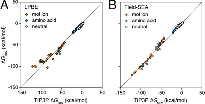
MD simulations of ΔGsolv for 504 neutral solutes (white), 35 molecular ions (orange), and 22 capped amino acid dipeptides (cyan) in TIP3P water, compared to (A) LPBE and (B) field-SEA.
Figure S5 (SI) compares the total solvation free energy from field-SEA with experimental results. The MSE/RMSE of field-SEA to experimental solvation free energy (0.67/1.45 kcal/mol, Table S6 (SI)) is comparable to that of the much more computationally expensive TIP3P water model (0.66/1.22 kcal/mol).52 These results indicate that field-SEA can accurately compute solvation free energies over the full range from charge-dense ions to neutral polar and nonpolar molecular solutes.
3.4. Solvation of Polyatomic Ions
Here, we test field-SEA on an expanded set of molecular ions and biomolecules (e.g., acetate, butylammonium, etc.; see SI Table S7 for the complete list and results).53−56 These are ions that are larger and more complex than the simple atomic and diatomic ions described above and should better test the need for adaptive boundary considerations.
Figure 5 compares solvation energies from LPBE (orange diamond) and field-SEA (orange circle; see SI Figure S6 for field-SEA results with a fixed rw boundary) with TIP3P results for 35 molecular ions. The errors for both LPBE and field-SEA with a fixed rw boundary are around 10 kcal/mol (Table 1). While this might be regarded as acceptable in light of the nearly 100 kcal/mol span of free energies covered in the TIP3P simulations, using an adaptive boundary with field-SEA has half of this RMSE. Field-SEA also performs well in multivalent molecular ion solvation (SI Figure S7) and is as accurate as explicit-solvent calculations compared to experimental values for ionic solute solvation (Table S6 and Figure S8, SI).
3.5. Solvation of Dipeptides
We also tested our methods on 22 capped amino acids (N-acetyl-X-methylamide, X = Glu, Arg, Leu, etc.; SI Table S8), which are widely used biological models in both theoretical studies57 and experiments.58 These are useful precursor structures for the foundation of hydrophobicity scales, used in estimating the solvation of larger biomolecular structures.58−61 Here, we investigate the solvation free energies of a full series of capped amino acids with field-SEA. As the size of solute increases, computing the total solvation free energy usually becomes increasingly intractable in explicit water. Implicit models become more useful for large systems. As Table 1 and Figure 5 show, LPBE (cyan diamond) and field-SEA (cyan circle) both yield solvation free energies that agree well with TIP3P calculations. Again, the adaptive boundary helps field-SEA considerably, cutting the RMSE to half of that seen from the LPBE or fixed rw cases. These results indicate that the accuracy of field-SEA does not degrade as the solute size further increases.
3.6. Sensitivity of Boundary Detail in Molecular Solvation
The solvation boundaries in field-SEA are made from a set of surface dots. The more dots, the slower the calculation. In the calculations above, we used 80 dots/atom, the same as was used in previous SEA studies.37,38 What is the minimum number of grid dots that we need to properly represent the first-shell boundary? To investigate this, we performed an analysis of accuracy versus relative computational time as a function of the granularity of the boundary. This analysis indicates that the RMSE for field-SEA results on the 504 neutral molecule set is essentially uncompromised even down to a granularity of 5 dots/atom, without increasing the RMSE above 1 kcal/mol (Figure S9 and S10 (SI), the granularity does not affect the accuracy for charged solutes either). At 5 dots/atom, field-SEA is roughly 5-fold faster than dipolar SEA at 80 dots/atom, the minimum surface granularity recommended for this method.38 These results indicate that while field-SEA is sensitive to the physicality of the solvation boundary, it is less sensitive to the granularity of its depiction.
4. Conclusions
We have described field-SEA, a method for computing solvation free energies of solutes in water. It improves upon an earlier method called SEA (semi-explicit assembly). SEA captured the physics of solvation by presimulating toy spheres in explicit water, collecting a database of structural and energetic properties of those waters and then assembling at run time the solvation physics as sums over appropriate toy spheres to properly represent a given solute. In field-SEA, this procedure differs in using a solvation free-energy field, rather than explicit waters. Furthermore, field-SEA uses an adaptive boundary, allowing solvating waters to approach a solute atom to different degrees depending on neighboring atoms. Relative to SEA, field-SEA captures the solvation free energies of ions and charged solutes accurately, is faster to compute, and has no degradation of performance on nonpolar and polar solutes. Both SEA and field-SEA offer advantages over implicit-solvent modeling in that they entail no adjustable solute atom radii parameters. SEA and field-SEA are built upon a corresponding force field and explicit-solvation model. Here, we use the TIP3P explicit water model.
One of the key observations that arises from our MD simulations of charged solutes in TIP3P water, which is captured by field-SEA, is that atoms that are adjacent to charged atoms in solutes acquire partial characteristics of those charged atoms. For example, a weakly charged atom’s solvation shell is shrunk by its neighboring big charges. An implication of this for implicit-solvent modeling is that atomic radii should not be treated as fixed for solvation in water; an atom’s radius in implicit-solvent modeling can depend on the nature of its neighboring atom.
Acknowledgments
We dedicate this paper to Bill Swope, who has been such a great pioneer, mentor, and gentleman to us and so many others. The authors gratefully acknowledge financial support provided by NIH Grant GM63592. We also appreciate valuable discussions with Robert C. Rizzo and Gabriel Rocklin about molecular ion solvation free-energy calculations.
Supporting Information Available
Details of explicit-solvent simulations and LPBE solvation calculations with references and calculated solvation energies (LPBE, fixed rw field-SEA, etc.) for solutes investigated in this study. This material is available free of charge via the Internet at http://pubs.acs.org.
The authors declare no competing financial interest.
Funding Statement
National Institutes of Health, United States
Supplementary Material
References
- Roux B.; Simonson T. Implicit Solvent Models. Biophys. Chem. 1999, 78, 1–20. [DOI] [PubMed] [Google Scholar]
- Feig M.; Brooks C. L. Recent Advances in the Development and Application of Implicit Solvent Models in Biomolecule Simulations. Curr. Opin. Struct. Biol. 2004, 14, 217–224. [DOI] [PubMed] [Google Scholar]
- Cramer C. J.; Truhlar D. G. Implicit Solvation Models: Equilibria, Structure, Spectra, and Dynamics. Chem. Rev. 1999, 99, 2161–2200. [DOI] [PubMed] [Google Scholar]
- Villa A.; Mark A. E. Calculation of the Free Energy of Solvation for Neutral Analogs of Amino Acid Side Chains. J. Comput. Chem. 2002, 23, 548–553. [DOI] [PubMed] [Google Scholar]
- Shirts M. R.; Pitera J. W.; Swope W. C.; Pande V. S. Extremely Precise Free Energy Calculations of Amino Acid Side Chain Analogs: Comparison of Common Molecular Mechanics Force Fields for Proteins. J. Chem. Phys. 2003, 119, 5740–5761. [Google Scholar]
- Mobley D. L.; Dumont E.; Chodera J. D.; Dill K. A. Comparison of Charge Models for Fixed-Charge Force Fields: Small-Molecule Hydration Free Energies in Explicit Solvent. J. Phys. Chem. B 2007, 111, 2242–2254. [DOI] [PubMed] [Google Scholar]
- Still W. C.; Tempczyk A.; Hawley R. C.; Hendrickson T. Semianalytical Treatment of Solvation for Molecular Mechanics and Dynamics. J. Am. Chem. Soc. 1990, 112, 6127–6129. [Google Scholar]
- Cramer C. J.; Truhlar D. G. An SCF Solvation Model for the Hydrophobic Effect and Absolute Free-Energies of Aqueous Solvation. Science 1992, 256, 213–217. [DOI] [PubMed] [Google Scholar]
- Luo R.; David L.; Gilson M. K. Accelerated Poisson–Boltzmann Calculations for Static and Dynamic Systems. J. Comput. Chem. 2002, 23, 1244–1253. [DOI] [PubMed] [Google Scholar]
- Guthrie J. P. A Blind Challenge for Computational Solvation Free Energies: Introduction and Overview. J. Phys. Chem. B 2009, 113, 4501–4507. [DOI] [PubMed] [Google Scholar]
- Rizzo R. C.; Aynechi T.; Case D. A.; Kuntz I. D. Estimation of Absolute Free Energies of Hydration Using Continuum Methods: Accuracy of Partial, Charge Models and Optimization Of Nonpolar Contributions. J. Chem. Theory Comput. 2006, 2, 128–139. [DOI] [PubMed] [Google Scholar]
- Honig B.; Nicholls A. Classical Electrostatics in Biology and Chemistry. Science 1995, 268, 1144–1149. [DOI] [PubMed] [Google Scholar]
- Kehoe C. W.; Fennell C. J.; Dill K. A. Testing the Semi-Explicit Assembly Solvation Model in the SAMPL3 Community Blind Test. J. Comput.-Aided Mol. Des. 2012, 26, 563–568. [DOI] [PubMed] [Google Scholar]
- Jorgensen W. L.; Chandrasekhar J.; Madura J. D.; Impey R. W.; Klein M. L. Comparison of Simple Potential Functions for Simulating Liquid Water. J. Chem. Phys. 1983, 79, 926–935. [Google Scholar]
- Ren P. Y.; Ponder J. W. Polarizable Atomic Multipole Water Model for Molecular Mechanics Simulation. J. Phys. Chem. B 2003, 107, 5933–5947. [Google Scholar]
- Onufriev A.; Bashford D.; Case D. A. Modification of the Generalized Born Model Suitable for Macromolecules. J. Phys. Chem. B 2000, 104, 3712–3720. [Google Scholar]
- Eisenberg D.; Mclachlan A. D. Solvation Energy in Protein Folding and Binding. Nature 1986, 319, 199–203. [DOI] [PubMed] [Google Scholar]
- Ooi T.; Oobatake M.; Nemethy G.; Scheraga H. A. Accessible Surface-Areas As a Measure of the Thermodynamic Parameters of Hydration of Peptides. Proc. Natl. Acad. Sci. U.S.A. 1987, 84, 3086–3090. [DOI] [PMC free article] [PubMed] [Google Scholar]
- Lazaridis T.; Karplus M. Effective Energy Function for Proteins in Solution. Proteins 1999, 35, 133–152. [DOI] [PubMed] [Google Scholar]
- Wang J. M.; Wang W.; Huo S. H.; Lee M.; Kollman P. A. Solvation Model Based on Weighted Solvent Accessible Surface Area. J. Phys. Chem. B 2001, 105, 5055–5067. [Google Scholar]
- Boyer R. D.; Bryan R. L. Fast Estimation of Solvation Free Energies for Diverse Chemical Species. J. Phys. Chem. B 2012, 116, 3772–3779. [DOI] [PubMed] [Google Scholar]
- Mobley D. L.; Barber A. E.; Fennell C. J.; Dill K. A. Charge Asymmetries in Hydration of Polar Solutes. J. Phys. Chem. B 2008, 112, 2405–2414. [DOI] [PMC free article] [PubMed] [Google Scholar]
- Chorny I.; Dill K. A.; Jacobson M. P. Surfaces Affect Ion Pairing. J. Phys. Chem. B 2005, 109, 24056–24060. [DOI] [PubMed] [Google Scholar]
- Fennell C. J.; Dill K. A. Physical Modeling of Aqueous Solvation. J. Stat. Phys. 2011, 145, 209–226. [DOI] [PMC free article] [PubMed] [Google Scholar]
- Florian J.; Warshel A. Calculations of Hydration Entropies of Hydrophobic, Polar, and Ionic Solutes in the Framework of the Langevin dipoles Solvation Model. J. Phys. Chem. B 1999, 103, 10282–10288. [Google Scholar]
- Marrink S. J.; de Vries A. H.; Mark A. E. Coarse Grained Model for Semiquantitative Lipid Simulations. J. Phys. Chem. B 2004, 108, 750–760. [Google Scholar]
- King G.; Warshel A. A Surface Constrained All-Atom Solvent Model for Effective Simulations of Polar Solutions. J. Chem. Phys. 1989, 91, 3647–3661. [Google Scholar]
- Beglov D.; Roux B. Finite Representation of an Infinite Bulk System — Solvent Boundary Potential for Computer-Simulations. J. Chem. Phys. 1994, 100, 9050–9063. [Google Scholar]
- Im W.; Berneche S.; Roux B. Generalized Solvent Boundary Potential for Computer Simulations. J. Chem. Phys. 2001, 114, 2924–2937. [Google Scholar]
- Lee M. S.; Salsbury F. R.; Olson M. A. An Efficient Hybrid Explicit/Implicit Solvent Method for Biomolecular Simulations. J. Comput. Chem. 2004, 25, 1967–1978. [DOI] [PubMed] [Google Scholar]
- Hummer G. Hydrophobic Force Field as a Molecular Alternative to Surface-Area Models. J. Am. Chem. Soc. 1999, 121, 6299–6305. [Google Scholar]
- Okur A.; Wickstrom L.; Layten M.; Geney R.; Song K.; Hornak V.; Simmerling C. Improved Efficiency of Replica Exchange Simulations through Use of a Hybrid Explicit/Implicit Solvation Model. J. Chem. Theory Comput. 2006, 2, 420–433. [DOI] [PubMed] [Google Scholar]
- Geney R.; Layten M.; Gomperts R.; Hornak V.; Simmerling C. Investigation of Salt Bridge Stability in a Generalized Born Solvent Model. J. Chem. Theory Comput. 2006, 2, 115–127. [DOI] [PubMed] [Google Scholar]
- Hummer G.; Garde S.; Garcia A. E.; Pohorille A.; Pratt L. R. An Information Theory Model of Hydrophobic Interactions. Proc. Natl. Acad. Sci. U.S.A. 1996, 93, 8951–8955. [DOI] [PMC free article] [PubMed] [Google Scholar]
- Du Q. H.; Beglov D.; Roux B. Solvation Free Energy of Polar and Nonpolar Molecules in Water: An Extended Interaction Site Integral equation Theory in Three Dimensions. J. Phys. Chem. B 2000, 104, 796–805. [Google Scholar]
- Wagoner J. A.; Baker N. A. Assessing Implicit Models for Nonpolar Mean Solvation Forces: The Importance of Dispersion and Volume Terms. Proc. Natl. Acad. Sci. U.S.A. 2006, 103, 8331–8336. [DOI] [PMC free article] [PubMed] [Google Scholar]
- Fennell C. J.; Kehoe C.; Dill K. A. Oil/Water Transfer Is Partly Driven by Molecular Shape, Not Just Size. J. Am. Chem. Soc. 2010, 132, 234–240. [DOI] [PMC free article] [PubMed] [Google Scholar]
- Fennell C. J.; Kehoe C. W.; Dill K. A. Modeling Aqueous Solvation with Semi-Explicit Assembly. Proc. Natl. Acad. Sci. U.S.A. 2011, 108, 3234–3239. [DOI] [PMC free article] [PubMed] [Google Scholar]
- Baker N. A.; Sept D.; Joseph S.; Holst M. J.; McCammon J. A. Electrostatics of Nanosystems: Application to Microtubules and the Ribosome. Proc. Natl. Acad. Sci. U.S.A. 2001, 98, 10037–10041. [DOI] [PMC free article] [PubMed] [Google Scholar]
- Lee B.; Richards F. M. Interpretation of Protein Structures — Estimation of Static Accessibility. J. Mol. Biol. 1971, 55, 379. [DOI] [PubMed] [Google Scholar]
- Latimer W. M.; Pitzer K. S.; Slansky C. M. The Free Energy of Hydration of Gaseous Ions, and the Absolute Potential of the Normal Calomel Electrode. J. Chem. Phys. 1939, 7, 108–111. [Google Scholar]
- Rajamani S.; Ghosh T.; Garde S. Size Dependent Ion Hydration, Its Asymmetry, and Convergence to Macroscopic Behavior. J. Chem. Phys. 2004, 120, 4457–4466. [DOI] [PubMed] [Google Scholar]
- Purisima E. O.; Sulea T. Restoring Charge Asymmetry in Continuum Electrostatics Calculations of Hydration Free Energies. J. Phys. Chem. B 2009, 113, 8206–8209. [DOI] [PubMed] [Google Scholar]
- Mukhopadhyay A.; Fenley A. T.; Tolokh I. S.; Onufriev A. V. Charge Hydration Asymmetry: The Basic Principle and How to Use It to Test and Improve Water Models. J. Phys. Chem. B 2012, 116, 9776–9783. [DOI] [PMC free article] [PubMed] [Google Scholar]
- Aqvist J. Ion Water Interaction Potentials Derived from Free-Energy Perturbation Simulations. J. Phys. Chem. 1990, 94, 8021–8024. [Google Scholar]
- Joung I. S.; Cheatham T. E. Determination of Alkali and Halide Monovalent Ion Parameters for use in Explicitly Solvated Biomolecular Simulations. J. Phys. Chem. B 2008, 112, 9020–9041. [DOI] [PMC free article] [PubMed] [Google Scholar]
- Hou G. H.; Zhu X. A.; Cui Q. A. An Implicit Solvent Model for SCC-DFTB with Charge-Dependent Radii. J. Chem. Theory Comput. 2010, 6, 2303–2314. [DOI] [PMC free article] [PubMed] [Google Scholar]
- Onufriev A.; Case D. A.; Bashford D. Effective Born Radii in the Generalized Born Approximation: The Importance of Being Perfect. J. Comput. Chem. 2002, 23, 1297–1304. [DOI] [PubMed] [Google Scholar]
- Thomas D. G.; Chun J.; Chen Z.; Wei G. W.; Baker N. A. Parameterization of a Geometric Flow Implicit Solvation Model. J. Comput. Chem. 2013, 34, 687–695. [DOI] [PMC free article] [PubMed] [Google Scholar]
- Dzubiella J.; Swanson J. M. J.; McCammon J. A. Coupling Nonpolar and Polar Solvation Free Energies in Implicit Solvent Models. J. Chem. Phys. 2006, 124, 084905. [DOI] [PubMed] [Google Scholar]
- Mobley D. L.; Dill K. A.; Chodera J. D. Treating Entropy and Conformational Changes in Implicit Solvent Simulations of Small Molecules. J. Phys. Chem. B 2008, 112, 938–946. [DOI] [PMC free article] [PubMed] [Google Scholar]
- Mobley D. L.; Bayly C. I.; Cooper M. D.; Shirts M. R.; Dill K. A. Small Molecule Hydration Free Energies in Explicit Solvent: An Extensive Test of Fixed-Charge Atomistic Simulations. J. Chem. Theory Comput. 2009, 5, 350–358. [DOI] [PMC free article] [PubMed] [Google Scholar]
- Lew S.; Caputo G. A.; London E. The Effect of Interactions Involving Ionizable Residues Flanking Membrane-Inserted Hydrophobic Helices upon Helix–Helix Interaction. Biochemistry 2003, 42, 10833–10842. [DOI] [PubMed] [Google Scholar]
- Tombola F.; Pathak M. M.; Isacoff E. Y. How Does Voltage Open an Ion Channel?. Annu. Rev. Cell Dev. Biol. 2006, 22, 23–52. [DOI] [PubMed] [Google Scholar]
- Nakase I.; Takeuchi T.; Tanaka G.; Futaki S. Methodological and Cellular Aspects That Govern the Internalization Mechanisms of Arginine-Rich Cell-Penetrating Peptides. Adv. Drug Delivery Rev. 2008, 60, 598–607. [DOI] [PubMed] [Google Scholar]
- Li L. B.; Vorobyov I.; Allen T. W. Potential of Mean Force and pKa Profile Calculation for a Lipid Membrane-Exposed Arginine Side Chain. J. Phys. Chem. B 2008, 112, 9574–9587. [DOI] [PubMed] [Google Scholar]
- Wimley W. C.; Creamer T. P.; White S. H. Solvation Energies of Amino Acid Side Chains and Backbone in a Family of Host–Guest Pentapeptides. Biochemistry 1996, 35, 5109–5124. [DOI] [PubMed] [Google Scholar]
- Wimley W. C.; White S. H. Experimentally Determined Hydrophobicity Scale for Proteins at Membrane Interfaces. Nat. Struct. Biol. 1996, 3, 842–848. [DOI] [PubMed] [Google Scholar]
- Nozaki Y.; Tanford C. Solubility of Amino Acids and 2 Glycine Peptides in Aqueous Ethanol and Dioxane Solutions — Establishment of a Hydrophobicity Scale. J. Biol. Chem. 1971, 246, 2211. [PubMed] [Google Scholar]
- Wolfenden R.; Andersson L.; Cullis P. M.; Southgate C. C. B. Affinities of Amino-Acid Side-Chains for Solvent Water. Biochemistry 1981, 20, 849–855. [DOI] [PubMed] [Google Scholar]
- Sitkoff D.; Sharp K. A.; Honig B. Accurate Calculation of Hydration Free-Energies Using Macroscopic Solvent Models. J. Phys. Chem. 1994, 98, 1978–1988. [Google Scholar]
Associated Data
This section collects any data citations, data availability statements, or supplementary materials included in this article.