

Abstract
We introduce a framework for population analysis of white matter tracts based on diffusion-weighted images of the brain. The framework enables extraction of fibers from high angular resolution diffusion images (HARDI); clustering of the fibers based partly on prior knowledge from an atlas; representation of the fiber bundles compactly using a path following points of highest density (maximum density path; MDP); and registration of these paths together using geodesic curve matching to find local correspondences across a population. We demonstrate our method on 4-Tesla HARDI scans from 565 young adults to compute localized statistics across 50 white matter tracts based on fractional anisotropy (FA). Experimental results show increased sensitivity in the determination of genetic influences on principal fiber tracts compared to the tract-based spatial statistics (TBSS) method. Our results show that the MDP representation reveals important parts of the white matter structure and considerably reduces the dimensionality over comparable fiber matching approaches.
Keywords: HARDI, tractography, MRI, brain, clustering, atlas, Dijkstra, shortest path, geodesic distance, Hough, connectivity, maximum density path, curve registration, longest path
Introduction
Diffusion weighted imaging (DWI) measures the directional diffusion of water through the brain in vivo. By following the dominant directions of diffusion across the brain, whole-brain tractography algorithms can reconstruct the brain’s major white matter pathways, extracting a vast number of fibers that are amenable to statistical analysis. We can then study these white matter regions in individuals and populations to better understand disease effects (Takahashi et al., 2002; Jahanshad et al., 2012b; Daianu et al., 2013), changes in brain microstructure and connectivity with age (Abe et al., 2002; Dennis et al., 2012), hemispheric differences (Jahanshad et al., 2010), sex differences (Peled et al., 1998), and genetic influences (Kochunov et al., 2010; Jahanshad et al., 2013b).
High angular resolution diffusion imaging (HARDI) enables a more accurate representation of fiber directions compared to the more standard single-tensor model (Basser and Pierpaoli, 1996). The single-tensor model does not account for fiber crossing or mixing, but the orientation distribution function (ODF) (Tuch, 2004) can be derived from HARDI images to discriminate multiple fibers with different orientations passing through a voxel (Leow et al., 2009; Zhan et al., 2010).
The large number of fibers generated by the tractography algorithms first need to be clustered according to known anatomical pathways before comparing them across subjects. A wealth of clustering methods have been applied to tractography results including fuzzy clustering (Shimony et al., 2002), normalized cuts (Brun et al., 2004), k-means (O’Donnell and Westin, 2005), spectral clustering (O’Donnell et al., 2006), Dirichlet distributions (Maddah et al., 2008), hierarchical clustering (Visser et al., 2011), a Gaussian process framework (Wassermann et al., 2010b), and median filtering (Prasad et al., 2011a). Some of these methods readily benefit from prior anatomical information provided by an atlas of likely locations of the tracts in the brain (Yendiki et al., 2011), suggesting when to split or combine clusters to conform to known anatomy. In one approach (Jin et al., 2011a,b, 2013), several labeled atlases are deformed onto a fiber set extracted from a new subject, and a fiber matching and voting process is used to help decide the anatomical bundles to which the fibers belong.
Following clustering, several methods can be used for fiber bundle matching. Colby et al. (2011) use a parametric curve-based method to resample fibers in a bundle based on shared seed points and then compute correspondences from the resampling to create a representative path for an individual or group. A similar re-sampling approach is used in a method (Yeatman et al., 2012) that filters fiber bundles to match a probabilistic atlas. Corouge et al. (2006) analyze fiber bundles by resampling and then aligning them across subjects using Procrustes analysis (Goodall, 1991) to generate a mean shape. Roberts et al. (2005) apply a density measure derived from tractography results. Their measure (fiber density index; FDi) quantifies the average number of detected fiber paths passing through voxels in a ROI. Wassermann et al. (2010a) use Gaussian processes to create voxel-wise probability maps of white matter structure. The fiber locations in high density regions of the image space are used by O’Donnell et al. (2009) as a template to align other fibers and compute correspondences. Yushkevich et al. (2008) analyze white matter tracts using deformable geometric medial models that allow for integration of nearby tensor-based features to reduce the dimensionality and improve registration. Patel et al. (2010) use a fast-marching algorithm to encapsulate white matter tracts in voxel based boundaries, which are then matched using variational techniques.
In contrast to the parameterized methods mentioned above, white matter analysis can also be performed using a voxel-based approach. A popular method known as tract based spatial statistics (TBSS) (Smith et al., 2006), uses a skeletonized representation of white matter and uses nonlinear registration for matching the skeletons. Although it is a very popular approach, TBSS does not explicitly represent tracts that would be recognized by anatomists, and therefore is not guaranteed to produce a consistent labeling of tracts from one brain to another (Schwarz et al., 2013). Although voxel-based methods can also be used to analyze DWI, they are often sensitive to the image registration (Tustison et al., 2012). Most existing white matter analysis techniques focus on nonlinear registration of fractional anisotropy (FA) images as in TBSS (Smith et al., 2006) and voxel-based morphometry (VBM), which can be applied to DWI-derived maps such as FA (Jones et al., 2005). Other approaches that focus on diffusion tensor correspondences are usually based on a global image registration (Wang et al., 2011b; Yeo et al., 2009), but a high-dimensional registration of tensor fields may also be used, as can tensor-based statistics (Chiang et al., 2008; Lepore et al., 2008; Lee et al., 2009). Given the richness of information provided by tractography, it seems advantageous to directly study the fiber tract bundles rather than simply analyzing voxel-based representation.
Approach
Our work adopts a parameterized approach by refining the representation of white matter structure into compact and localized paths, represented as 3D curves. These paths represent the most influential regions in tractography and are used as compact dimensional representations of the fiber bundle. Our method uses an additional local registration of specific white matter regions to fix biases (Tustison et al., 2012) in voxel-based analysis and many of the problems of registration algorithms (Klein et al., 2009) that work on the entire image. Additionally, our approach may offer increased statistical power as it finds shape homologies across different white matter tracts.
Termed the maximum density path (MDP) approach, it incorporates information from tractography-derived fibers by selecting a subset of fiber bundles from a white matter atlas in the same space. We generate a density image from the fiber bundles and use it to create a graph with voxel locations as nodes and fiber density measures as edges. We implement a widely used graph search algorithm to find the MDP between two pre-specified regions of interest (ROI) in the atlas. The MDPs represent fiber bundles that characterize a tract using points of highest density. These compact descriptions of a tract’s scale, location, and high-level geometric information are computed for all subjects in a population. We find correspondences across the paths by bringing them into the same space using geodesic curve registration. Finally, the average MDP for a given population is computed using a nonlinear iterative method. As an example, we use our method to determine genetic influences on white matter tracts based on a large cohort of over 565 twin subjects scanned using HARDI at 4-Tesla. We compare the results to those obtained by the more standard TBSS method.
MDPs have been used as one tool for pilot studies of sex differences and a variety of diseases (Prasad et al., 2011b; Nir et al., 2012). In the current study we explicate the technical details of the method, validate its repeatability, compare it to the widely used TBSS, and use MDPs to study heritability along with genetic associations. The main contributions of this work are as follows:
Fiber tract bundles are represented by compact reduced dimensional representations known as maximum density paths (MDPs).
MDPs are represented by vector valued functions and are analyzed in an intrinsic and invariant manner.
Shape matching between MDPs is achieved using geodesic curve registration that not only yields smooth deformations between MDPs, but also provides shape distances between them.
Group analysis of MDPs is conveniently performed using an intrinsic statistical framework that enables the computation of shape averages and their first order variations.
Fiber bundle analysis via MDPs is used to identify highly heritable regions in the white matter tissues in twin subjects and is also used to show genetic associations.
Materials and Methods
This section describes important steps starting with the extraction of fibers using HARDI tractography, clustering of fibers using a white matter ROI atlas, representation and matching of fiber bundles using MDPs, and finally, statistical analysis of MDPs in a population. The schematic pipeline outlining the extraction and representation of MDPs is shown in Figure 1, whereas the workflow for statistical group analysis is shown in Figure 2.
Figure 1.

Schematic of the pipeline for extraction, clustering, and representation of maximum density paths (MDPs) for a single subject. The first panel shows the fibers from our HARDI global tractrography method. The co-registered region of interest (ROI) atlas is used to select a fiber bundle representing a particular white matter tract. The resulting fiber bundle is then converted to a volumetric density image, which is transformed into a graph. Selected seed points in the image form the nodes of the graph, that are used to compute maximum density paths. The maximum density path compactly summarizes a given white matter structure and enables specific matching of these regions across subjects using curve registration.
Figure 2.

Schematic of the pipeline for performing statistical analysis of populations of MDPs. The first panel represents MDPs for a population of subjects for a given white matter tract. A nonlinear iterative method that uses geodesic curve registrations is used to compute an average MDP representing the mean shape of the population. A correspondence is established for all subject MDPs via the average MDP. Fractional anisotropy (FA) from each subject is resampled for the corresponding points and compared across the population.
HARDI Tractography using the Hough Transform
We use a global tractography algorithm (Aganj et al., 2011) to extract fibers from HARDI images.
The algorithm uses extensive information provided by HARDI at each voxel, parametrized by the orientation distribution function (ODF).
Our tractography method selects fibers in the diffusion image space by generating scores for all possible curves at a seed point. These curves are parameterized using 2nd order polynomials. An additional parameter controls the maximum expected curve length and is set to a value representing the largest dimension of the volume. In practice, the number of curves evaluated at each seed point is around one million based on resolution and computational resources.
First, seed points are generated using a prior probability based on FA from the single-tensor model of diffusion (Basser and Pierpaoli, 1996), defined as
| (1) |
where λ1, λ2, and λ3 are the eigenvalues of the diffusion tensor. These seed points are used to generate curves that receive a score estimating the probability of their existence, computed from the voxels the curve passes through.
The ODFs at each voxel from our HARDI images were computed using a normalized and dimensionless estimator derived from Q-ball imaging (QBI) (Aganj et al., 2010). This method uses the Jacobian factor r2 for the constant solid angle (CSA) ODF as
| (2) |
In this equation, is the diffusion signal, S0 is the baseline image, FRT is the Funk-Radon transform, and is the Laplace-Beltrami operator. This estimate outperforms the original definition (Tuch, 2004) with superior resolution for detecting multiple fiber orientations (Aganj et al., 2010; Fritzsche et al., 2010; Descoteaux and Bore, 2012; Ghosh et al., 2013).
The Hough transform tractography chooses fibers from all possible curves generated in the image at a certain space and parameter resolution. These curves are parametrized by their arc length, s, ranging in value from L− to L+ and approximated using simple polynomials. The scores for each possible curve, s, derive from the ODF and FA values
| (3) |
where is the value from the ODF at the 3D location and direction specified by the unit tangent vector . The method scores as many fibers as possible arising from a seed point and uses the voting process provided by the Hough transform to select the best fitting curve. These filtered curves comprise the final set of fibers produced by the method for a single subject, which we refer to as F.
The method is probabilistic in its selection of a fiber at a certain seed point but does not generate volumetric data giving a distribution of fibers in the white matter. It chooses seed points (voxel locations) randomly throughout the white matter tissue with a probability proportional to their fractional anisotropy. Once a seed point is chosen, the algorithm scores all possible fibers that pass through this point. The number of fibers is restricted by the parameterization and range of the variables involved, but is close to one million candidate fibers. For each fiber this score represents the probability of that fiber existing and is constructed by integrating the orientation distribution function over the span of the fiber combined with the probability of the corresponding seed point. The method then uses the Hough transform to select the fiber with the highest probability or highest score as the final fiber for that seed point.
The tractography algorithm was run on each subject image and generated around 10,000 fibers (Fig. 1 shows a representative example with our data), which represents a good balance between computational efficiency and sampling enough of the image space (Prasad et al., 2013c). We subsequently clustered these fibers using a white matter atlas.
Fiber Clustering with White Matter ROI Atlas
Fibers extracted using the Hough transform-based tractography method are clustered using a ROI atlas to incorporate prior anatomical information. We use the Johns Hopkins University (JHU) atlas (Wakana et al., 2004), which delineates 50 white matter regions of interest (ROI). This ROI atlas is first registered to our subject space using an affine transform provided by FMRIB’s Linear Image Registration Tool (FLIRT) (Jenkinson and Smith, 2001). This is then followed by a nonlinear transform from the Automatic Registration Toolbox (ART) (Klein et al., 2009; Ardekani et al., 2005) to refine the registration further.
We then cluster the fiber bundles by measuring the intersection of fibers with the ROI atlas as follows. A fiber intersection score is computed by counting the number of ROI voxels that intersect with the fiber tract. This score is used to select fibers that belong to an ROI and thus a white matter tract. Spuriously intersecting fibers are eliminated by applying an experimentally determined threshold that is dependent on the number and the type of fibers obtained from the tractography algorithm. Formally, if F is the set of fibers for a subject and r is a specific white matter ROI label in the atlas, then the subset of selected fibers in a bundle is given by,
| (4) |
where t is the intersection threshold and A is an indicator function defined to be
| (5) |
Bundle Representation using the Maximum Density Path
The fiber bundle B representing a white matter tract is reduced to a compact representation also referred to as the maximum density path as follows. We first compute a density volume of our fiber bundle to characterize our search space, and denote it as
| (6) |
where represents a 3D voxel location and Q is the indicator function
| (7) |
This value specifies the number of fibers that intersect each voxel. We then construct a graph that represents the voxel-wise fiber density in our fiber bundle. The above voxels are used as nodes in a graph, G = {N, E} (a set of nodes and undirected edges connecting them) with those of positive value connected to their 26 neighbors by undirected edges. In our formulation, the weight of an edge between nodes i and j is calculated as the sum of the voxel densities it connected as
| (8) |
with as the density for the voxel location corresponding to node k. These edge weights are then modified by subtracting each from the maximum initial edge cost, em, such that edges in high density regions have weights close to zero. These edge weights are designed to allow the shortest path algorithm to go through edges in high density regions. We use Dijkstra’s algorithm (Dijkstra, 1959) to compute the path through this graph following the nodes with highest density. Dijkstra’s algorithm is a graph search method that finds the shortest path from a source node to every other node. However, the number of nodes in the graph may be large and when the algorithm is used for a single destination node, it may be stopped once that path is found. To find the shortest path to represent a white matter region, we require the graph to have start and end nodes to constrain the path to a specific region of the graph. These nodes are specified by an expert in the ROI atlas. The ROI points for the start and end locations may not always correspond to the positive density values derived from our bundle. Thus, we find the closest voxels in the density volume as the corresponding start and end nodes in subsequent computation with Euclidean distance used as the metric.
In our implementation, we used Dijkstra’s algorithm (Dijkstra, 1959) to only find the shortest path between the start and the end nodes selected in the graph. If Dijkstra’s algorithm is unable to find the path between the start and end nodes our method automatically identifies this situation and takes steps to remedy the graph and find the shortest path. The algorithm will be incapable of finding a connection between the two nodes if the structure of the graph is such that there are no edges from the subgraph containing the start node with the subgraph containing the end node. This can be caused by scanner artifacts or suboptimal solutions due to the fiber tractrography algorithm. In this situation, we add extra edges and nodes to the graph so all voxels within our ROI are fully connected with their neighbors. The edges are weighted by the largest edge cost in the current graph. This allows gaps between the start and end nodes to be filled in and use as few edges as possible in regions with unknown data. The nodes in the path correspond to a set of voxel locations in our image space. We smooth the path so it is better conditioned for subsequent processing. We convolve the 3D coordinates of our path with a Gaussian kernel to achieve this, though fitting these points to a spline would also have sufficed. A summary of these steps is presented in Algorithm 1. We represent the maximum density path by the coordinate function of the parameterized curve, and denote it to be β such that . Figure 3 shows an example of a maximum density path computed for a fiber bundle. Additionally, we show the density and the FA images that correspond to the fibers. For comparison, we also show a representative mean fiber by applying Procrustes analysis to align the fibers in the bundle to their mean. We then compute a new mean (shown in blue) of the fibers after alignment. This example shows that even if the bundle includes a few spurious fibers, it can drastically change the appearance of the mean fiber derived from Procrustes analysis, while the MDP remains stable. Figure 5 shows an example of MDPs for a population of subjects overlaid on each other. Some of these paths are short because the corresponding regions of interest in the white matter atlas are small. This means the seed points specified in the atlas are not very far apart and even if the fibers are much larger they are summarized by the structure within the white matter region and points with the highest density. An alternative could be to use a probabilistic white matter atlas and threshold the regions so they encompass a larger fraction of the fiber lengths in the white matter region.
Figure 3.

This figure shows the advantage of using the maximum density path method to represent fiber bundles. The first panel shows the tractography fibers that intersect a white matter tract. The selected fibers all intersect the region of interest to the same degree, but the selection process includes spurious fibers. In the context of fractional anisotropy, we can see that the spurious fibers may be part of another adjacent tract. Our method represents the fiber bundle as a density image and searches for a representative path based on seed points from a registered atlas. The final slide shows the resulting maximum density path compared to a path found by taking the mean of the fibers and using Procrustes analysis to align and recompute a representative mean. If only the fiber shape is used, the resulting representative path from Procrustes analysis may not effectively traverse the region of interest due to spuriously included fibers. By leveraging the distribution of fibers the MDPs seek to build a representation of the white matter that is reflective of the underlying feature geometry of the most important regions and help matching across subjects for subsequent population analysis.
Figure 5.

We show here the maximum density paths (MDPs) computed for 238 subjects in 67 regions from the white matter atlas before they are matched together using curve registration. This sample was used for our heritability analysis. The color represents the direction or orientation of the middle segment connecting two points at the middle of each MDP. If the orientation is anterior to posterior it is colored green, if it is from left to right it is red, and if it is superior to inferior it is colored blue. In each of the 67 areas, we register the 238 MDPs to a mean MDP to find correspondences using geodesic curve registration. We then sample FA along corresponding points in each subject for our subsequent statistical and genetic analysis. A few of these paths are relatively short because the corresponding region of interest in the white matter atlas was small and thus the MDP will cover a shorter range even though the tractography fibers it represents may be much larger.
| Algorithm 1 Maximum Density Path Method |
|---|
| 1: Generate fibers from tractography |
| 2: for r = 1 to M (number of atlas regions) do |
| 3: for f = 1 to N (number of fibers) do |
| 4: Find intersection of fiber f and region r |
| 5: If intersection measure ∫f
A(s, r)ds > t add to bundle B |
| 6: end for |
| 7: Convert fiber bundle, B, to density image |
| 8: Generate graph G{N,E} with density image voxels as nodes and edge weights as em – (Id(i) + Id(j)) |
| 9: Find the closest (in Euclidean distance) start, a, and end, b, nodes from region r in the atlas |
| 10: Use Dijkstra’s algorithm to find the shortest path, p, between nodes a and b |
| 11: Convolve p with a Gaussian kernel to generate the maximum density path (MDP), β |
| 12: end for |
Shape Analysis of Maximum Density Paths
This section outlines the method for shape representation and analysis for maximum density paths. The maximum density paths denoting tracts are modeled as continuous open curves in but they can also be considered as points in an infinite-dimensional space of curves. This space is induced by a suitable Riemannian metric defined on its tangent space. Shape matching between MDPs is enabled by measuring shortest length paths, also known as geodesics connecting two shapes in the shape space. The geodesic not only measures the length of the path and quantifies the geometric distance between two shapes, but also represents an optimal geometric deformation that highlights the anatomical differences between the shapes. Additionally geodesics are an important ingredient for constructing intrinsic population averages for shapes - an essential step in statistical analysis of shapes.
Representation of MDPs
We represent the shape of the coordinate function of the MDP using a vector-valued function (Joshi et al., 2007a,b; Srivastava et al., 2011) as
| (9) |
Here, s ∈ [0, 1], and is the standard Euclidean product in . Our goal is to achieve an elastic shape matching between MDPs. We would also prefer that the shape matching is invariant with respect to the orientation and scale of the MDPs. Owing to the derivative, the function q is invariant to the translation of the MDP coordinate curve. To impose scale-invariance, we normalize the q functions by its magnitude. Thus we denote as the space of all unit-length curves. On account of scale invariance, the space becomes an infinite-dimensional unit-sphere of functions, and represents all open elastic curves invariant to translation and uniform scaling. The elasticity of the representation is due to the presence of the square-root in the denominator, that allows the q function to have arbitrary speeds. To define a metric on the space , we first define its tangent space which is the set of all tangent vectors orthogonal to q. Formally, the tangent space of is given by , ∀s ∈ [0,1] such that , where n = 3. Here each wi represents a tangent vector in the tangent space of . Now, the metric on the tangent space is defined as follows. Given a curve , and the first order perturbations of q given by , respectively, the inner product between the tangent vectors u, v to at q is defined as,
| (10) |
Now given two shapes q1 and q2, the translation and scale-invariant shape distance between them is simply found by measuring the length of the geodesic, or the great circle connecting them on the sphere. Thus given a tangent vector in the direction of q2 given by f = q2 – ⟨q1, q2⟩q1, the geodesic (Joshi et al., 2007a) on between the two points along f, for an infinitesimal time t is given by
| (11) |
Then the geodesic distance between the two shapes q1 and q2 is given by
| (12) |
The geodesic distance (Joshi et al., 2007a) given in Eqn. 12 is only invariant to translation and scale. To make it invariant to rotations, we consider the shortest distance
| (13) |
Eqn. 13 can be minimized either using gradient descent over the tangent space of SO(3) or by using singular value decomposition (Rohlf and Slice, 1990). In this paper, we find the rotation invariant distance as
| (14) |
where , A and B are left and right unitary matrices, and D is a matrix given by . Finally, since we are representing MDPs by parameterized curves, we would like the shape matching to be invariant to reparameterizations. Following Joshi et al. (2007a), we denote the reparameterization of a MDP curve using a group action by a diffeomorphism γ, given by . Then the optimal reparameterization is approximated by the minimizer
| (15) |
where . In this paper, we use dynamic programming to obtain the solution to Eq. 15. The fully elastic, pose, scale, and reparameterization invariant distance between MDPs is given by
| (16) |
The optimal geodesic path can also be denoted by a one-parameter flow Ψ and the tangent vector , such that
| (17) |
The optimal tangent vector can then be written from Eqn. 17 as
| (18) |
Statistical analysis of MDPs across a Population
To evaluate group-level effects of sex, age, disease or even genetic influences on the MDP representations of white matter tracts, we need a suitable mechanism for performing statistical analysis. As MDPs are represented by parameterized functions defined on a shape space, one natural approach is to use the inherent non-linearity of the shape space, and define appropriate statistical measures under the Riemannian metric in Eqn. 10. This approach is also called an intrinsic statistical analysis and leads to the definition of the Karcher mean (also known as the Fréchet mean) (Le, 1995; Srivastava et al., 2005; Joshi et al., 2013) in the shape space of all MDPs. Given a collection of MDP shapes {qi}, i = 1, …, N, the Karcher mean is defined as
| (19) |
The computation of the Karcher mean involves computing geodesics at each step iteratively and proceeds as follows. For the first iteration, an extrinsic mean (Euclidean average) is computed and projected on the shape space. This is assumed to be the current estimate of the Karcher mean. For the subsequent iterations, geodesics are computed between all the individual shapes in the population to the current estimate. The tangent vectors are then computed as a result of minimizing Eqn. 16 and averaged together. A geodesic flow is then constructed using Eqn. 17 to yield a new estimate of the mean shape. This procedure is repeated until the geodesic variance given by the sum of the squared geodesic distances to the mean shape is minimized, and the mean converges. The Karcher mean completely relies on the geometry of the shape space and is useful in computing intrinsic statistical estimates such as covariances of MDPs. Additionally, the geodesics produce correspondences, making it easier to compare white matter measures projected on the MDPs across a population. This is also useful for studying differences in disease, sex, aging, or even heritability in a population.
Results
Experiments
We show experimental results on a dataset of N = 565 young adults, including healthy twins and their siblings. The participants were scanned with a 4-Tesla Bruker Medspec MRI scanner, collecting 3D 105-gradient high angular resolution diffusion images (HARDI) and standard structural T1-weighted magnetic resolution images (MRI). The images consisted of 55 slices, 2-mm thick, with a 1.79 × 1.79 mm2 in-plane resolution. For each person, we collected 94 diffusion-weighted images (b = 1159 s/mm2) using a uniform distribution of gradient directions on the hemisphere. We also collected 11 b0 (non-diffusion encoding) images and corrected all images for eddy current distortions and motion with FSL (www.fmrib.ox.ax.uk/fsl). Our cohort consisted of 367 women and 198 men, ranging from 20 to 29 years of age. Study participants gave informed consent; institutional ethics committees at the Queensland Institute of Medical Research, the university of Queensland, the Wesley Hospital, and at UCLA approved the study.
For each T1-weighted image, we manually removed non-brain tissue and registered it to the Colin27 (Holmes et al., 1998) high resolution brain template using a 9-parameter transformation. These skull-stripped and registered T1-weighted images each have a corresponding average b0 diffusion weighted image (DWI), combining all the eleven images. These average images were masked using BET (Smith, 2002) and this space was used to generate FA maps. Additionally, we used the FA images to compute a geometrically-centered study-specific mean template (mean deformation template; MDT). We registered the JHU ROI atlas to the MDT for the MDP analysis. Our ROI atlas contained 50 different white matter regions, which were seeded to extract 67 different MDPs. Our results based on all 565 subjects are shown in Figure 6.
Figure 6.

Average maximum density paths (MDPs) for 67 fiber bundles in 565 twin images. The color represents the direction or orientation of the middle segment connecting two points at the middle of each MDP. If the orientation is anterior to posterior it is colored green, if it is from left to right it is red, and if it is superior to inferior it is colored blue. The paths are derived from tractography fibers, clustered into white matter tracts, and then represented as paths that follow points in these white matter bundles of maximum density of fibers. The 67 different paths come from regions in our white matter atlas that have been annotated with seed points, which become the endpoints of the paths. The mean MDPs provide a template for curve registration to find correspondences between the individual subjects and allow us to compactly represent population statistics across the entire white matter.
Repeatability of MDPs
We examined the reliability of the MDP construction procedure by analyzing subjects with repeat scans. Twenty-three subjects in the total population used in our analysis had repeat scans, which were used to test the stability of MDP construction across the two acquisitions. We used the MDP algorithm to find corresponding points along each MDP and used paired-sample t-tests to study if the FA values in these white matter tract representations were significantly different. Figure 4 shows the collection of MDPs with 46 curves in each white matter region from the ROI atlas. Each of the 23 pairs is colored randomly with the two MDPs in a single pair having matching coloring. We corrected for multiple comparisons using the false discover rate (FDR) (Benjamini and Hochberg, 1995) at the 0.05 level and none of the values were significantly different between scans. This provides an indication of the stability of MDP representation and may help support a more meaningful interpretation of the subsequent statistical analyses.
Figure 4.
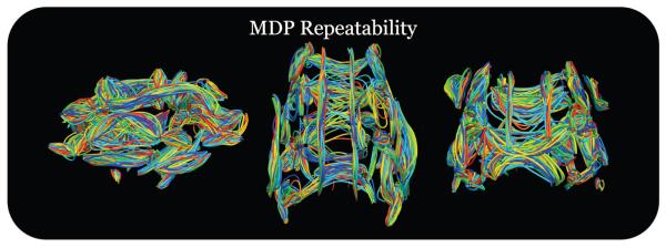
To study the variability of the maximum density paths (MDPs), we used 23 subjects with repeat scans. We used the MDP algorithm to represent 67 white matter regions from an ROI atlas and find correspondences between the two acquisitions for a single subject. We used paired-sample t-tests to compare the fractional anisotropy (FA) values across corresponding points. We found that there were no significant differences in the MDPs when correcting for multiple comparisons using the false discovery rate (FDR) at the 0.05 level. This helps provide support that the statistical analysis tools using MDPs will be able to investigate patterns of white matter structure and may be less affected by noisy or highly variable representation inherent to the algorithm.
Genetic effects on white matter morphology using MDPs
The twin cohort in the data is made up of monozyogotic (MZ) and dizygotic (DZ) pairs, allowing us to estimate the relative contributions of additive genetic factors (A), shared environment (C), and unshared or unique environment (E) to the measures derived from the scans - in our case, FA along the MDPs. This standard “A/C/E” model describes the FA at each point on the MDP as a combination of latent variables, FA = aA + cC + eE. In this formulation the total variance is var(FA) = a2 + c2 + e2 with var(A) = a2, var(C) = c2, and var(E) = e2. We are able to estimate the unobserved factor loadings as there is a difference in the theoretical covariance of FA for a MZ twin pair, a2 + c2, and for a DZ twin pair, (1/2)a2 + c2, which we solved using a maximum likelihood fitting (Neale and Cardon, 1992) that estimated the parameters of the model. These methods are detailed in (Chiang et al., 2009).
Several studies (Chiang et al., 2011; Patel et al., 2010; Thompson et al., 2001; Jahanshad et al., 2013a) have shown evidence for heritability of the white matter structure in the brain. Here, we use heritability as a metric to understand how well MDPs were able to model and capture the underlying morphology of the white matter structure in our data. If the representation is able to effectively pick up heritability effects then our hypothesis is that the MDP matching across subjects reflects the underlying anatomical homology, and that the MDP model is better able to describe white matter brain structure.
We fitted the “A/C/E” model to the FA values on the skeleton that fell within the ROI atlas. In our experiments we compared the full “A/C/E” model to the simpler formulation with two variables using minus two times the log-likelihood ratio, which approximately follows a χ2 distribution, meaning that P > 0.05 indicates a good fit. We found that the shared environment term (C component) did not have a significant fit for either method, so we used a simplified “A/E” model instead. This model selection procedure and selecting the “A/E” model instead of the more complicated “A/C/E” is widely used (Geschwind et al., 2002) and common with real data (Baaré et al., 2001). In the “A/E” model, a2 represents the proportion of the variance due to additive genetic factors and the other parameter in the model, e2, represents the proportion of variance that is due to environmental factors including measurement error. Thus we model the components of FA variance as simply var(FA) = a2 + e2 and since we are interested in the relative proportion of variance captured by each component we can normalize this equation by var(FA) to interpret their relationship as or . The goal here is to use the model that best fits the data to understand the genetic and environmental contributions to the variance. Maximizing heritable estimates in this case may imply minimizing measurement error and therefore may represent a stronger metric for measuring white matter microstructure. In addition, these highly heritable regions present good candidates for genetic associations and could be useful for cutting down on the dimensionality of the image for these types of analyses.
We also compared our method of analyzing white matter bundles using MDPs and analyzing the white matter skeletons from TBSS (Figure 7) in our subjects. We used the genetic contribution due to FA using both methods to compare heritability. We found that the density and FA images smoothed with an isotropic Gaussian filter with full-width at half maximum (FWHM) = 3 mm produced higher a2 values (Chiang et al., 2012). We restricted the analysis to 238 (48 monozygotic and 71 dizygotic) of the 565 twins because of issues with the nonlinear registration from TBSS in the omitted subjects.
Figure 7.

Our twin data contained monozygotic (MZ) twins that share 100% of their genetic material and dizygotic twins (DZ) that share 50% of their genetic material. This structure in our data allows us to use structural equation models, particularly the A/E model, to estimate the amount of variance in a phenotype (in our case the white matter structure) that is due to genetic effects (heritability), or to unique environment factors and measurement error. In this figure we show the genetic contribution to white matter structure using our maximum density (MDP) path representation method compared with the white matter skeleton from tract-based spatial statistics (TBSS). A high value (red) means a large fraction of the variance in white matter structure is determined by genetic effects while a low value (blue) means the variance in structure was accounted for more by the environment. Since this is the proportion of variance accounted for by heritability, an analogous figure of the environmental contributions would involve simply reversing the color bar. Previous studies have shown high heritability of white matter tissue and we used the fraction of genetic determination as the metric to evaluate how well our MDP representation summarized the white matter structure in our data. The MDP method may have a better ability to pick up on the heritability because of the curve registration that is computed for each white matter region individually, which improves coherence of homologous points across subjects. We used a subset of 238 subjects for this analysis (48 MZ pairs, 71 DZ pairs). The top panel shows the MDPs from 67 white matter regions with slices of the atlas overlaid. The TBSS results show orthogonal slices of the TBSS skeleton overlaid on the white matter atlas.
We computed genetic associations with mixed-model regression (Jahanshad et al., 2012a; Aulchenko et al., 2007) along the MDPs using the genes NTRK1, CLU, and COMT. We found NTRK1 passed a local false discovery rate (FDR) threshold (for a single MDP) in 20 regions across our white matter atlas represented as MDPs. In addition, we found CLU passed local FDR at the anterior limb of internal capsule right, posterior limb of internal capsule right, and anterior corona radiata left, and COMT passed at the sagittal stratum right (including inferior longitidinal fasciculus and inferior fronto-occipital fasciculus). When we used a global FDR, by combining the 67 MDPs into one large MDP, NTRK1 was the only SNP that survived in 600 of the total 1897 points in the global MDP. The results from NTRK1 and CLU agree with earlier studies of this dataset using voxel-based maps (Braskie et al., 2012, 2011).
Discussion and Conclusion
We have presented a method for extracting, representing, and analyzing the geometry of white matter bundles using maximum density paths. Our method enables population analysis of diffusion-weighted images without relying exclusively on global registration of the images into the same space. Image registration is performed only once to transform the ROI white matter atlas to the subject space for the purpose of initializing the seed points for clustering fibers from tractography. Density image volumes are computed from the fiber bundles, and MDPs are constructed using Dijkstra’s algorithm by imposing a graph structure on the images. The shapes of MDPs are then brought into correspondence through geodesic curve registration, allowing us to focus specifically on the white matter region we are interested in without involving the rest of the image. Further, our method introduces a way to perform localized statistical analysis of white matter tracts. The MDPs, use the start and end points from major white matter pathways, and provide a compact representation so that correspondences can be easily computed. The correspondences can be directly visualized on the MDPs to reveal which part of a white matter tract depends on an external parameter. These tools provide the foundation for any study of white matter tracts or any type of population analysis using diffusion weighted images. The complete procedure is available as a end-to-end computational pipeline for white matter tract-based analysis of diffusion images.
In the examples presented here, we used a global Hough transform method for tractography, but the MDP representation is general enough to be used with any type of tractography method. Our method relies on density images from tractography, which could be computed using streamlines (Basser et al., 2000), a deflection based algorithm (Lazar et al., 2003), or any of the recent deterministic and probabilistic methods (Zhan et al., 2013). In our case, we chose a tractography method that could benefit from the information rich HARDI data, but depending on the resources and data available, researchers may prefer to use fibers from diffusion tensor imaging or diffusion spectrum imaging (Wedeen et al., 2005) based algorithms. The graph-based representation for the fiber density volume led to conveniently incorporating the density information in the structure, and further led to an efficient solution provided by Dijkstra’s algorithm. However we could have formulated the problem using snakes (Kass et al., 1988) or splines (Park and Lee, 2007) as well. Alternatively, other density representations such as those using surfaces (Zijdenbos et al., 1994) or using the volumetric segmentations (Kubicki et al., 2005) directly would have introduced a host of issues with registration and subsequent analysis of correspondences. We chose to use an ROI atlas to select fibers for analysis and representation with the MDP though alternative approaches may work without relying on the registration of the atlas into the image space. Future work could incorporate automatic clustering of tractography fibers using approaches such as a hierarchical Dirichlet processes mixture model (Wang et al., 2011a), a voxel based approach (Guevara et al., 2011), a spectral approach (Guevara et al., 2011), or even shape clustering (Joshi and Srivastava, 2003; Joshi et al., 2004). Hierarchical approaches may enable a user to specify the resolution of MDPs in the brain tissue. As an alternative to FA, any other type of statistics on the density paths could be used instead. We could compute mean diffusivity (Le Bihan et al., 2001), generalized FA (Barmpoutis et al., 2009), or the tensor distribution function and interpolate them along each MDP. Our white matter analysis framework could even be scored by their capacity (Prasad et al., 2013b) and used as measures of connectivity to complement (Prasad et al., 2013a) and optimize our representation of brain connectivity networks (Prasad et al., 2014).
Preliminary studies have used MDPs to study sex differences (Prasad et al., 2011b), Alzheimer’s disease (Nir et al., 2012, 2014), 22q11.2 deletion syndrome (Villalon-Reina et al., 2012), and depression (Sacchet et al., 2014). Our results in the current study showed promise in our new representation and agreed with voxelwise analyses of the entire white matter tissue in diffusion images (Chiang et al., 2011; Patel et al., 2010; Thompson et al., 2001; Jahanshad et al., 2013a) that showed a pattern of highly heritable regions. In this work, we evaluated MDPs by their ability to detect the effects of heritability in a cohort of monozyogitic and dizygotic twins. Heritability analysis of FA in 50 regions of interest delineated in an ROI atlas, suggested promise of the method for detecting other factors that affect tracts, such as disease and risk genes. When comparing the genetic contributions (Figure 7) to brain structure detected by our MDP method versus the TBSS method, we showed that MDPs can represent and display the structure using only one-tenth of the points in a TBSS skeleton. This reduction of the structural image data, which contains millions of voxels, may prove useful for genome-wise association studies (Stein et al., 2010; Cichon et al., 2009), as an alternative to voxel-based morphometry, or instead of group comparisons of statistics from segmentations. These data reduction steps may reduce the computational expense of a genome-wide search, and may also increase statistical power. In summary, we find that using tractography and creating MDPs gives a similar skeletonized, yet more neuroanatomically accurate estimate of white matter microstructure than does TBSS as we found through improved heritability measures in the same sample.
Fiber bundles represented by compact reduced dimensional paths.
Paths are vector functions and are analyzed in an intrinsic, invariant manner.
Shape matching between paths is achieved using geodesic curve registration.
Group analysis of paths enables shape averages and their first order variations.
Paths identify highly heritable parts of white matter tissue in a set of twins.
Acknowledgments
This study was supported by NIH R01 grants MH097268, NS080655, AG040060, and EB008432. Additional support was provided by the National Health and Medical Research Council (NHMRC 486682, 1009064), Australia. Genotyping was supported by NHMRC (389875).
Footnotes
Author Disclosure Statement: The authors have no competing financial interests.
Publisher's Disclaimer: This is a PDF file of an unedited manuscript that has been accepted for publication. As a service to our customers we are providing this early version of the manuscript. The manuscript will undergo copyediting, typesetting, and review of the resulting proof before it is published in its final citable form. Please note that during the production process errors may be discovered which could affect the content, and all legal disclaimers that apply to the journal pertain.
References
- Abe O, Aoki S, Hayashi N, Yamada H, Kunimatsu A, Mori H, Yoshikawa T, Okubo T, Ohtomo K. Normal aging in the central nervous system: Quantitative MR diffusion-tensor analysis. Neurobiology of Aging. 2002;23(3):433–441. doi: 10.1016/s0197-4580(01)00318-9. [DOI] [PubMed] [Google Scholar]
- Aganj I, Lenglet C, Jahanshad N, Yacoub E, Harel N, Thompson PM, Sapiro G. A Hough transform global probabilistic approach to multiple-subject diffusion MRI tractography. Medical Image Analysis. 2011;15(4):414–425. doi: 10.1016/j.media.2011.01.003. [DOI] [PMC free article] [PubMed] [Google Scholar]
- Aganj I, Lenglet C, Sapiro G, Yacoub E, Ugurbil K, Harel N. Reconstruction of the orientation distribution function in single-and multiple-shell Q-ball imaging within constant solid angle. Magnetic Resonance in Medicine. 2010;64(2):554–566. doi: 10.1002/mrm.22365. [DOI] [PMC free article] [PubMed] [Google Scholar]
- Ardekani B, Guckemus S, Bachman A, Hoptman M, Wojtaszek M, Nierenberg J, et al. Quantitative comparison of algorithms for inter-subject registration of 3D volumetric brain MRI scans. Journal of Neuroscience Methods. 2005;142(1):67–76. doi: 10.1016/j.jneumeth.2004.07.014. [DOI] [PubMed] [Google Scholar]
- Aulchenko Y, De Koning D, Haley C. Genomewide rapid association using mixed model and regression: A fast and simple method for genomewide pedigree-based quantitative trait loci association analysis. Genetics. 2007;177(1):577–585. doi: 10.1534/genetics.107.075614. [DOI] [PMC free article] [PubMed] [Google Scholar]
- Baaré W, Pol H, Boomsma D, Posthuma D, de Geus E, Schnack H, van Haren N, van Oel C, Kahn R. Quantitative genetic modeling of variation in human brain morphology. Cerebral Cortex. 2001;11(9):816–824. doi: 10.1093/cercor/11.9.816. [DOI] [PubMed] [Google Scholar]
- Barmpoutis A, Hwang M, Howland D, Forder J, Vemuri B. Regularized positive-definite fourth order tensor field estimation from DW-MRI. NeuroImage. 2009;45(1):S153–S162. doi: 10.1016/j.neuroimage.2008.10.056. [DOI] [PMC free article] [PubMed] [Google Scholar]
- Basser P, Pajevic S, Pierpaoli C, Duda J, Aldroubi A. In vivo fiber tractography using DT-MRI data. Magnetic Resonance in Medicine. 2000;44(4):625–632. doi: 10.1002/1522-2594(200010)44:4<625::aid-mrm17>3.0.co;2-o. [DOI] [PubMed] [Google Scholar]
- Basser P, Pierpaoli C. Microstructural and physiological features of tissues elucidated by quantitative-diffusion-tensor MRI. Journal of Magnetic Resonance-Series B. 1996;111(3):209–219. doi: 10.1006/jmrb.1996.0086. [DOI] [PubMed] [Google Scholar]
- Benjamini Y, Hochberg Y. Controlling the false discovery rate: a practical and powerful approach to multiple testing. Journal of the Royal Statistical Society. Series B (Methodological) 1995;57(1):289–300. [Google Scholar]
- Braskie M, Jahanshad N, Stein J, Barysheva M, Johnson K, McMahon K, de Zubicaray G, Martin N, Wright M, Ring-man J, et al. Relationship of a variant in the NTRK1 gene to white matter microstructure in young adults. The Journal of Neuroscience. 2012;32(17):5964–5972. doi: 10.1523/JNEUROSCI.5561-11.2012. [DOI] [PMC free article] [PubMed] [Google Scholar]
- Braskie M, Jahanshad N, Stein J, Barysheva M, McMahon K, de Zubicaray G, Martin N, Wright M, Ringman J, Toga A, et al. Common alzheimer’s disease risk variant within the clu gene affects white matter microstructure in young adults. The Journal of Neuroscience. 2011;31(18):6764–6770. doi: 10.1523/JNEUROSCI.5794-10.2011. [DOI] [PMC free article] [PubMed] [Google Scholar]
- Brun A, Knutsson H, Park H, Shenton M, Westin C. Clustering fiber traces using normalized cuts. Medical Image Computing and Computer-Assisted Intervention–MICCAI2004. 2004;7:368–375. doi: 10.1007/b100265. [DOI] [PMC free article] [PubMed] [Google Scholar]
- Chiang M, Barysheva M, McMahon K, de Zubicaray G, Johnson K, Montgomery G, Martin N, Toga A, Wright M, Shapshak P, et al. Gene network effects on brain microstructure and intellectual performance identified in 472 twins. The Journal of Neuroscience. 2012;32(25):8732–8745. doi: 10.1523/JNEUROSCI.5993-11.2012. [DOI] [PMC free article] [PubMed] [Google Scholar]
- Chiang M, Barysheva M, Shattuck D, Lee A, Madsen S, Avedissian C, Klunder A, Toga A, McMahon K, De Zubicaray G, et al. Genetics of brain fiber architecture and intellectual performance. Journal of Neuroscience. 2009;29(7):2212–2224. doi: 10.1523/JNEUROSCI.4184-08.2009. [DOI] [PMC free article] [PubMed] [Google Scholar]
- Chiang M, Leow A, Dutton R, Barysheva M, Rose S, McMahon K, de Zubicaray G, Toga A, Thompson P. Fluid Registration of Diffusion Tensor Images Using Information Theory. IEEE Transactions on Medical Imaging. 2008;27(4):442–456. doi: 10.1109/TMI.2007.907326. [DOI] [PMC free article] [PubMed] [Google Scholar]
- Chiang M, McMahon K, de Zubicaray G, Martin N, Hickie I, Toga A, Wright M, Thompson P. Genetics of white matter development: a DTI study of 705 twins and their siblings aged 12 to 29. NeuroImage. 2011;54(3):2308–2317. doi: 10.1016/j.neuroimage.2010.10.015. [DOI] [PMC free article] [PubMed] [Google Scholar]
- Cichon S, Craddock N, Daly M, Faraone S, Gejman P, Kelsoe J, Lehner T, Levinson D, Moran A, Sklar P, et al. Genomewide association studies: history, rationale, and prospects for psychiatric disorders. The American Journal of Psychiatry. 2009;166(5):540–556. doi: 10.1176/appi.ajp.2008.08091354. [DOI] [PMC free article] [PubMed] [Google Scholar]
- Colby J, Soderberg L, Lebel C, Dinov I, Thompson P, Sowell E. Along-tract statistics allow for enhanced tractography analysis. NeuroImage. 2011;59(4):3227–3242. doi: 10.1016/j.neuroimage.2011.11.004. [DOI] [PMC free article] [PubMed] [Google Scholar]
- Corouge I, Fletcher P, Joshi S, Gouttard S, Gerig G. Fiber tract-oriented statistics for quantitative diffusion tensor MRI analysis. Medical Image Analysis. 2006;10(5):786–798. doi: 10.1016/j.media.2006.07.003. [DOI] [PubMed] [Google Scholar]
- Daianu M, Jahanshad N, Nir T, Toga A, Jack C, Weiner M, Thompson P. Breakdown of brain connectivity between normal aging and Alzheimer’s disease: A structural k-core network analysis. Brain Connectivity. 2013;3(4) doi: 10.1089/brain.2012.0137. [DOI] [PMC free article] [PubMed] [Google Scholar]
- Dennis E, Jahanshad N, McMahon K, de Zubicaray G, Martin N, Hickie I, Toga A, Wright M, Thompson P. Development of brain structural connectivity between ages 12 and 30: A 4-Tesla diffusion imaging study in 439 adolescents and adults. NeuroImage. 2012 doi: 10.1016/j.neuroimage.2012.09.004. [DOI] [PMC free article] [PubMed] [Google Scholar]
- Descoteaux M, Bore A. Testing classical single-shell HARDI techniques. Biomedical Imaging: From Nano to Macro, 2012 IEEE International Symposium on (HARDI Reconstruction Workshop). IEEE.2012. p. 5. [Google Scholar]
- Dijkstra E. A note on two problems in connexion with graphs. Numerische Mathematik. 1959;1(1):269–271. [Google Scholar]
- Fritzsche KH, Laun FB, Meinzer H-P, Stieltjes B. Opportunities and pitfalls in the quantification of fiber integrity: What can we gain from Q-ball imaging? NeuroImage. 2010;51(1):242–251. doi: 10.1016/j.neuroimage.2010.02.007. [DOI] [PubMed] [Google Scholar]
- Geschwind D, Miller B, DeCarli C, Carmelli D. Heritability of lobar brain volumes in twins supports genetic models of cerebral laterality and handedness. Proceedings of the National Academy of Sciences. 2002;99(5):3176–3181. doi: 10.1073/pnas.052494999. [DOI] [PMC free article] [PubMed] [Google Scholar]
- Ghosh A, Tsigaridas E, Mourrain B, Deriche R. A polynomial approach for extracting the extrema of a spherical function and its application in diffusion MRI. Medical Image Analysis. 2013 doi: 10.1016/j.media.2013.03.004. [DOI] [PubMed] [Google Scholar]
- Goodall C. Procrustes methods in the statistical analysis of shape. Journal of the Royal Statistical Society: Series B (Methodological) 1991;53(2):285–339. [Google Scholar]
- Guevara P, Poupon C, Rivière D, Cointepas Y, Descoteaux M, Thirion B, Mangin J. Robust clustering of massive tractography datasets. NeuroImage. 2011;54(3):1975–1993. doi: 10.1016/j.neuroimage.2010.10.028. [DOI] [PubMed] [Google Scholar]
- Holmes C, Hoge R, Collins L, Woods R, Toga A, Evans A. Enhancement of MR images using registration for signal averaging. Journal of Computer Assisted Tomography. 1998;22(2):324–333. doi: 10.1097/00004728-199803000-00032. [DOI] [PubMed] [Google Scholar]
- Jahanshad N, Kochunov P, Sprooten E, Mandl R, Nichols T, Almassy L, Blangero J, Brouwer R, Curran J, de Zubicaray G, et al. Multi-site genetic analysis of diffusion images and voxelwise heritability analysis: A pilot project of the ENIGMA– DTI working group. NeuroImage. 2013a doi: 10.1016/j.neuroimage.2013.04.061. [DOI] [PMC free article] [PubMed] [Google Scholar]
- Jahanshad N, Kohannim O, Hibar D, Stein J, McMahon K, de Zubicaray G, Medland S, Montgomery G, Whitfield J, Martin N, et al. Brain structure in healthy adults is related to serum transferrin and the H63D polymorphism in the HFE gene. Proceedings of the National Academy of Sciences. 2012a;109(14):E851–E859. doi: 10.1073/pnas.1105543109. [DOI] [PMC free article] [PubMed] [Google Scholar]
- Jahanshad N, Lee A, Barysheva M, McMahon K, de Zubicaray G, Martin N, Wright M, Toga A, Thompson P. Genetic influences on brain asymmetry: A DTI study of 374 twins and siblings. NeuroImage. 2010;52(2):455–469. doi: 10.1016/j.neuroimage.2010.04.236. [DOI] [PMC free article] [PubMed] [Google Scholar]
- Jahanshad N, Rajagopalan P, Hua X, Hibar D, Nir T, Toga A, Jack C, Saykin A, Green R, Weiner M, et al. Genome-wide scan of healthy human connectome discovers SPON1 gene variant influencing dementia severity. Proceedings of the National Academy of Sciences. 2013b;110(12):4768–4773. doi: 10.1073/pnas.1216206110. [DOI] [PMC free article] [PubMed] [Google Scholar]
- Jahanshad N, Valcour V, Nir T, Kohannim O, Busovaca E, Nicolas K, Thompson P. Disrupted brain networks in the aging HIV+ population. Brain Connectivity. 2012b;2(6):335–344. doi: 10.1089/brain.2012.0105-Rev. [DOI] [PMC free article] [PubMed] [Google Scholar]
- Jenkinson M, Smith S. A global optimisation method for robust a ne registration of brain images. Medical Image Analysis. 2001;5(2):143–156. doi: 10.1016/s1361-8415(01)00036-6. [DOI] [PubMed] [Google Scholar]
- Jin Y, Shi Y, Jahanshad N, Aganj I, Sapiro G, Toga A, Thompson P. 3D elastic registration improves HARDI-derived fiber alignment and automated tract clustering. Biomedical Imaging: From Nano to Macro, 2011 IEEE International Symposium on. IEEE.2011a. pp. 822–826. [Google Scholar]
- Jin Y, Shi Y, Joshi SH, Jahanshad N, Zhan L, De Zubicaray GI, McMahon KL, Martin NG, Wright MJ, Toga AW, et al. Multimodal Brain Image Analysis. Springer; 2011b. Heritability of white matter fiber tract shapes: a hardi study of 198 twins; pp. 35–43. [DOI] [PMC free article] [PubMed] [Google Scholar]
- Jin Y, Shi Y, Zhan L, de Zubicaray G, McMahon K, Martin N, Wright M, Thompson P. Automatic HARDI white matter labeling by fusion of multiple tract atlases and its application to genetics. Biomedical Imaging: From Nano to Macro, 2013 IEEE International Symposium on. IEEE; 2013. pp. 512–515. [DOI] [PMC free article] [PubMed] [Google Scholar]
- Jones D, Symms M, Cercignani M, Howard R, et al. The effect of filter size on VBM analyses of DT-MRI data. NeuroImage. 2005;26(2):546–554. doi: 10.1016/j.neuroimage.2005.02.013. [DOI] [PubMed] [Google Scholar]
- Joshi S, Klassen E, Srivastava A, Jermyn I. A novel representation for Riemannian analysis of elastic curves in Rn. 2007 IEEE Conference on Computer Vision and Pattern Recognition; 2007a. pp. 1–7. [DOI] [PMC free article] [PubMed] [Google Scholar]
- Joshi S, Klassen E, Srivastava A, Jermyn I. Removing shape-preserving transformations in square-root elastic (SRE) framework for shape analysis of curves. Energy Minimization Methods in Computer Vision and Pattern Recognition; 2007b. pp. 387–398. [DOI] [PMC free article] [PubMed] [Google Scholar]
- Joshi S, Srivastava A. A geometric approach to shape clustering and learning. Statistical Signal Processing, 2003 IEEE Workshop on. IEEE.2003. pp. 302–305. [Google Scholar]
- Joshi S, Srivastava A, Mio W, Liu X. Computer Vision-ECCV 2004. Springer; 2004. Hierarchical organization of shapes for e cient retrieval; pp. 570–581. [Google Scholar]
- Joshi SH, Narr KL, Philips OR, Nuechterlein KH, Asarnow RF, Toga AW, Woods RP. Statistical shape analysis of the corpus callosum in schizophrenia. NeuroImage. 2013;64(1):547–559. doi: 10.1016/j.neuroimage.2012.09.024. [DOI] [PMC free article] [PubMed] [Google Scholar]
- Kass M, Witkin A, Terzopoulos D. Snakes: Active contour models. International Journal of Computer Vision. 1988;1(4):321–331. [Google Scholar]
- Klein A, Andersson J, Ardekani B, Ashburner J, Avants B, Chiang M, Christensen G, Collins D, Gee J, Hellier P, et al. Evaluation of 14 nonlinear deformation algorithms applied to human brain MRI registration. NeuroImage. 2009;46(3):786. doi: 10.1016/j.neuroimage.2008.12.037. [DOI] [PMC free article] [PubMed] [Google Scholar]
- Kochunov P, Glahn D, Lancaster J, Winkler A, Smith S, Thompson P, Almasy L, Duggirala R, Fox P, Blangero J. Genetics of microstructure of cerebral white matter using diffusion tensor imaging. NeuroImage. 2010;53(3):1109–1116. doi: 10.1016/j.neuroimage.2010.01.078. [DOI] [PMC free article] [PubMed] [Google Scholar]
- Kubicki M, Park H, Westin C, Nestor P, Mulkern R, Maier S, Niznikiewicz M, Connor E, Levitt J, Frumin M, et al. DTI and MTR abnormalities in schizophrenia: Analysis of white matter integrity. NeuroImage. 2005;26(4):1109–1118. doi: 10.1016/j.neuroimage.2005.03.026. [DOI] [PMC free article] [PubMed] [Google Scholar]
- Lazar M, Weinstein D, Tsuruda J, Hasan K, Arfanakis K, Meyerand M, Badie B, Rowley H, Haughton V, Field A, et al. White matter tractography using diffusion tensor deflection. Human Brain Mapping. 2003;18(4):306–321. doi: 10.1002/hbm.10102. [DOI] [PMC free article] [PubMed] [Google Scholar]
- Le H. Mean size-and-shapes and mean shapes: A geometric point of view. Advances in applied probability. 1995;27(1):44–55. [Google Scholar]
- Le Bihan D, Mangin J, Poupon C, Clark C, Pappata S, Molko N, Chabriat H. Diffusion tensor imaging: concepts and applications. Journal of Magnetic Resonance Imaging. 2001;13(4):534–546. doi: 10.1002/jmri.1076. [DOI] [PubMed] [Google Scholar]
- Lee A, Lepore N, Brun C, Barysheva M, Chou Y, Chiang M, Madsen S, McMahon K, de Zubicaray G, Wright M, Toga A, Thompson P. The multivariate A/C/E model and the genetics of fiber architecture. Biomedical Imaging: From Nano to Macro, 2009 IEEE International Symposium on. IEEE; 2009. pp. 125–128. [DOI] [PMC free article] [PubMed] [Google Scholar]
- Leow A, Zhu S, Zhan L, McMahon K, de Zubicaray G, Meredith M, Wright M, Toga A, Thompson P. The tensor distribution function. Magnetic Resonance in Medicine. 2009;61(1):205–214. doi: 10.1002/mrm.21852. [DOI] [PMC free article] [PubMed] [Google Scholar]
- Lepore N, Brun C, Chou Y, Chiang M, Dutton R, Hayashi K, Lu A, Lopez O, Aizenstein H, Toga A, Becker J, Thompson P. Generalized tensor-based morphometry of HIV/AIDS using multivariate statistics on deformation tensors. IEEE Transactions on Medical Imaging. 2008;27(1):129–141. doi: 10.1109/TMI.2007.906091. [DOI] [PMC free article] [PubMed] [Google Scholar]
- Maddah M, Zollei L, Grimson W, Wells W. Modeling of anatomical information in clustering of white matter fiber trajectories using dirichlet distribution. 2008 IEEE Conference on Computer Vision and Pattern Recognition Workshops; IEEE; 2008. pp. 1–7. [DOI] [PMC free article] [PubMed] [Google Scholar]
- Neale M, Cardon L. Methodology for genetic studies of twins and families. Springer; 1992. [Google Scholar]
- Nir T, Prasad G, Joshi S, Villalon J, Jahanshad N, Toga A, Jack C, Weiner M, Thompson P. Predicting future brain atrophy from DTI-based maximum density path analysis in mild cognitive impairment and Alzheimer’s disease. Medical Image Computing and Computer-Assisted Intervention Workshop on Novel Imaging Biomarkers for Alzheimer’s Disease and Related Disorders. 2012:178–189. [Google Scholar]
- Nir T, Villalon-Reina J, Prasad G, Jahanshad N, Joshi S, Toga A, Bernstein M, Jack CR, Jr., Weiner M, Thompson P. DTI-based maximum density path analysis and classification of Alzheimer’s disease. Neurobiology of Aging. 2014 doi: 10.1016/j.neurobiolaging.2014.05.037. [DOI] [PMC free article] [PubMed] [Google Scholar]
- O’Donnell L, Kubicki M, Shenton M, Dreusicke M, Grimson W, Westin C. A method for clustering white matter fiber tracts. American Journal of Neuroradiology. 2006;27(5):1032–1036. [PMC free article] [PubMed] [Google Scholar]
- O’Donnell L, Westin C. White matter tract clustering and correspondence in populations. Medical Image Computing and Computer-Assisted Intervention–MICCAI 2005. 2005;8:140–147. [PubMed] [Google Scholar]
- O’Donnell L, Westin C, Golby A. Tract-based morphometry for white matter group analysis. NeuroImage. 2009;45(3):832–844. doi: 10.1016/j.neuroimage.2008.12.023. [DOI] [PMC free article] [PubMed] [Google Scholar]
- Park H, Lee J. B-spline curve fitting based on adaptive curve refinement using dominant points. Computer-Aided Design. 2007;39(6):439–451. [Google Scholar]
- Patel V, Chiang M, Thompson P, McMahon K, de Zubicaray G, Martin N, Wright M, Toga A. Scalar connectivity measures from fast-marching tractography reveal heritability of white matter architecture. Biomedical Imaging: From Nano to Macro, 2010 IEEE International Symposium on. IEEE.2010. pp. 1109–1112. [Google Scholar]
- Peled S, Gudbjartsson H, Westin C, Kikinis R, Jolesz F. Magnetic resonance imaging shows orientation and asymmetry of white matter fiber tracts. Brain Research. 1998;780(1):27–33. doi: 10.1016/s0006-8993(97)00635-5. [DOI] [PubMed] [Google Scholar]
- Prasad G, Burkart J, Joshi S, Thompson P. A dynamical clustering model of brain connectivity inspired by the n-body problem. Medical Image Computing and Computer-Assisted Intervention Workshop on Multimodal Brain Image Analysis. 2013a:129–137. doi: 10.1007/978-3-319-02126-3_13. [DOI] [PMC free article] [PubMed] [Google Scholar]
- Prasad G, Jahanshad N, Aganj I, Lenglet C, Sapiro G, Toga A, Thompson P. Atlas-based fiber clustering for multi-subject analysis of high angular resolution diffusion imaging tractography. Biomedical Imaging: From Nano to Macro, 2011 IEEE International Symposium on. IEEE; 2011a. pp. 276–280. [DOI] [PMC free article] [PubMed] [Google Scholar]
- Prasad G, Joshi S, Jahanshad N, Villalon J, Aganj I, Lenglet C, Sapiro G, McMahon K, de Zubicaray G, Martin N, Wright M, Toga A, Thompson P. White matter tract analysis in 454 adults using maximum density paths. Medical Image Computing and Computer-Assisted Intervention Workshop on Computational Diffusion MRI. 2011b:1–12. [Google Scholar]
- Prasad G, Joshi S, Nir T, Toga A, Thompson P. Flow-based network measures of brain connectivity in Alzheimer’S disease. Biomedical Imaging (ISBI), 2013 IEEE 10th International Symposium on. IEEE; 2013b. pp. 258–261. [DOI] [PMC free article] [PubMed] [Google Scholar]
- Prasad G, Joshi S, Thompson P. Optimizing brain connectivity networks for disease classification using EPIC. Biomedical Imaging (ISBI), 2014 IEEE 11th International Symposium on. IEEE; 2014. pp. 1–4. [DOI] [PMC free article] [PubMed] [Google Scholar]
- Prasad G, Nir T, Toga A, Thompson P. Tractography density and network measures in Alzheimer’s disease. Biomedical Imaging (ISBI), 2013 IEEE 10th International Symposium on. IEEE; 2013c. pp. 692–695. [DOI] [PMC free article] [PubMed] [Google Scholar]
- Roberts T, Liu F, Kassner A, Mori S, Guha A. Fiber density index correlates with reduced fractional anisotropy in white matter of patients with glioblastoma. American Journal of Neuroradiology. 2005;26(9):2183–2186. [PMC free article] [PubMed] [Google Scholar]
- Rohlf F, Slice D. Extensions of the procrustes method for the optimal superimposition of landmarks. Systematic Biology. 1990;39(1):40–59. [Google Scholar]
- Sacchet M, Prasad G, Foland-Ross L, Joshi S, Hamilton J, Thompson P, Gotlib I. Characterizing white matter connectivity in major depressive disorder: automated fiber quantification and maximum density paths. Biomedical Imaging: From Nano to Macro, 2014 IEEE International Symposium on. IEEE; 2014. pp. 1–4. [DOI] [PMC free article] [PubMed] [Google Scholar]
- Schwarz C, Reid R, Gunter J, Senjem M, Przybelski S, Zuk S, Whitwell J, Vemuri P, Josephs K, Kantarci1 K, Thompson P, Weiner M, Petersen R, Jr., C. J, Initiative, A. D. N. Improved DTI registration allows voxel-based analysis that outperforms tract-based spatial statistics. NeuroImage. 2013 doi: 10.1016/j.neuroimage.2014.03.026. [DOI] [PMC free article] [PubMed] [Google Scholar]
- Shimony J, Snyder A, Lori N, Conturo T. Automated fuzzy clustering of neuronal pathways in diffusion tensor tracking. Proc. Intl. Soc. Mag. Reson. Med. 2002;Vol. 10:1–1. [Google Scholar]
- Smith S. Fast robust automated brain extraction. Human Brain Mapping. 2002;17(3):143–155. doi: 10.1002/hbm.10062. [DOI] [PMC free article] [PubMed] [Google Scholar]
- Smith S, Jenkinson M, Johansen-Berg H, Rueckert D, Nichols T, Mackay C, Watkins K, Ciccarelli O, Cader M, Matthews P, et al. Tract-based spatial statistics: Voxelwise analysis of multi-subject diffusion data. NeuroImage. 2006;31(4):1487–1505. doi: 10.1016/j.neuroimage.2006.02.024. [DOI] [PubMed] [Google Scholar]
- Srivastava A, Joshi S, Mio W, Liu X. Statistical shape analysis: Clustering, learning, and testing. IEEE Transactions on Pattern Analysis and Machine Intelligence. 2005;27(4):590–602. doi: 10.1109/TPAMI.2005.86. [DOI] [PubMed] [Google Scholar]
- Srivastava A, Klassen E, Joshi SH, Jermyn I. Shape analysis of elastic curves in euclidean spaces. IEEE Transactions on Pattern Analysis and Machine Intelligence. 2011;33(7):1451–1428. doi: 10.1109/TPAMI.2010.184. [DOI] [PubMed] [Google Scholar]
- Stein J, Hua X, Lee S, Ho A, Leow A, Toga A, Saykin A, Shen L, Foroud T, Pankratz N, et al. Voxelwise genome-wide association study (vGWAS) NeuroImage. 2010;53(3):1160–1174. doi: 10.1016/j.neuroimage.2010.02.032. [DOI] [PMC free article] [PubMed] [Google Scholar]
- Takahashi S, Yonezawa H, Takahashi J, Kudo M, Inoue T, Tohgi H. Selective reduction of diffusion anisotropy in white matter of Alzheimer’s disease brains measured by 3.0 Tesla magnetic resonance imaging. Neuroscience Letters. 2002;332(1):45–48. doi: 10.1016/s0304-3940(02)00914-x. [DOI] [PubMed] [Google Scholar]
- Thompson P, Cannon T, Narr K, Van Erp T, Poutanen V, Huttunen M, Lönnqvist J, Standertskjöld-Nordenstam C, Kaprio J, Khaledy M, et al. Genetic influences on brain structure. Nature Neuroscience. 2001;4(12):1253–1258. doi: 10.1038/nn758. [DOI] [PubMed] [Google Scholar]
- Tuch D. Q-ball imaging. Magnetic Resonance in Medicine. 2004;52(6):1358–1372. doi: 10.1002/mrm.20279. [DOI] [PubMed] [Google Scholar]
- Tustison N, Avants B, Cook P, Kim J, Whyte J, Gee J, Stone J. Logical circularity in voxel-based analysis: Normalization strategy may induce statistical bias. Human Brain Mapping. 2012:1–15. doi: 10.1002/hbm.22211. [DOI] [PMC free article] [PubMed] [Google Scholar]
- Villalon-Reina J, Prasad G, Joshi S, Jalbrzikowski M, Toga A, Bearden C, Tompson P. Statistical analysis of maximum density path deformation fields in white matter tracts. Medical Image Computing and Computer-Assisted Intervention Workshop on Novel Imaging Biomarkers for Alzheimer’s Disease and Related Disorders.2012. pp. 198–209. [Google Scholar]
- Visser E, Nijhuis E, Buitelaar J, Zwiers M. Partition-based mass clustering of tractography streamlines. NeuroImage. 2011;54(1):303–312. doi: 10.1016/j.neuroimage.2010.07.038. [DOI] [PubMed] [Google Scholar]
- Wakana S, Jiang H, Nagae-Poetscher L, van Zijl P, Mori S. Fiber tract–based atlas of human white matter anatomy. Radiology. 2004;230(1):77–87. doi: 10.1148/radiol.2301021640. [DOI] [PubMed] [Google Scholar]
- Wang X, Grimson W, Westin C. Tractography segmentation using a hierarchical Dirichlet processes mixture model. NeuroImage. 2011a;54(1):290–302. doi: 10.1016/j.neuroimage.2010.07.050. [DOI] [PMC free article] [PubMed] [Google Scholar]
- Wang Y, Gupta A, Liu Z, Zhang H, Escolar M, Gilmore J, Gouttard S, Fillard P, Maltbie E, Gerig G, et al. DTI registration in atlas based fiber analysis of infantile Krabbe disease. NeuroImage. 2011b;55(4):1577–1586. doi: 10.1016/j.neuroimage.2011.01.038. [DOI] [PMC free article] [PubMed] [Google Scholar]
- Wassermann D, Bloy L, Kanterakis E, Verma R, Deriche R. Unsupervised white matter fiber clustering and tract probability map generation: Applications of a Gaussian process framework for white matter fibers. NeuroImage. 2010a;51(1):228–241. doi: 10.1016/j.neuroimage.2010.01.004. [DOI] [PMC free article] [PubMed] [Google Scholar]
- Wassermann D, Kanterakis E, Gur R, Deriche R, Verma R. Diffusion-based population statistics using tract probability maps. Medical Image Computing and Computer-Assisted Intervention–MICCAI2010. 2010b;13:631–639. doi: 10.1007/978-3-642-15705-9_77. [DOI] [PubMed] [Google Scholar]
- Wedeen V, Hagmann P, Tseng W, Reese T, Weissko R. Mapping complex tissue architecture with diffusion spectrum magnetic resonance imaging. Magnetic Resonance in Medicine. 2005;54(6):1377–1386. doi: 10.1002/mrm.20642. [DOI] [PubMed] [Google Scholar]
- Yeatman J, Dougherty R, Myall N, Wandell B, Feldman H. Tract profiles of white matter properties: automating fiber-tract quantification. PloS One. 2012;7(11):1–15. doi: 10.1371/journal.pone.0049790. [DOI] [PMC free article] [PubMed] [Google Scholar]
- Yendiki A, Panneck P, Srinivasan P, Stevens A, Zöllei L, Augustinack J, Wang R, Salat D, Ehrlich S, Behrens T, et al. Automated probabilistic reconstruction of white-matter pathways in health and disease using an atlas of the underlying anatomy. Frontiers in Neuroinformatics. 2011:5. doi: 10.3389/fninf.2011.00023. [DOI] [PMC free article] [PubMed] [Google Scholar]
- Yeo B, Vercauteren T, Fillard P, Peyrat J, Pennec X, Golland P, Ayache N, Clatz O. DT-REFinD: Diffusion tensor registration with exact finite-strain differential. Medical Imaging, IEEE Transactions on. 2009;28(12):1914–1928. doi: 10.1109/TMI.2009.2025654. [DOI] [PMC free article] [PubMed] [Google Scholar]
- Yushkevich P, Zhang H, Simon T, Gee J. Structure-specific statistical mapping of white matter tracts. NeuroImage. 2008;41(2):448–461. doi: 10.1016/j.neuroimage.2008.01.013. [DOI] [PMC free article] [PubMed] [Google Scholar]
- Zhan L, Jahanshad N, Jin Y, Toga A, McMahon K, Martin N, Wright M, de Zubicaray G, Thompson P. Brain network e ciency and topology depend on the fiber tracking method: 11 tractography algorithms compared in 536 subjects. IEEE International Symposium on Biomedical Imaging, ISBI 2013. IEEE.2013. pp. 1134–1137. [Google Scholar]
- Zhan L, Leow A, Jahanshad N, Chiang M, Barysheva M, Lee A, Toga A, McMahon K, de Zubicaray G, Wright M, et al. How does angular resolution affect diffusion imaging measures? NeuroImage. 2010;49(2):1357–1371. doi: 10.1016/j.neuroimage.2009.09.057. [DOI] [PMC free article] [PubMed] [Google Scholar]
- Zijdenbos A, Dawant B, Margolin R, Palmer A. Morpho-metric analysis of white matter lesions in MR images: method and validation. Medical Imaging, IEEE Transactions on. 1994;13(4):716–724. doi: 10.1109/42.363096. [DOI] [PubMed] [Google Scholar]