Keywords in the mental lexicon

Abstract

Network science draws from a number of fields to examine complex systems using nodes to represent individuals and connections to represent relationships between individuals to form a network. This approach has been used in several areas of Psychology to illustrate the influence that the structure of a network has on processing in that system. In the present study the concept of keyplayers in a network (Borgatti, 2006) was examined in the domain of Psycholinguistics. Keyplayers are nodes in a network that, when removed, result in the network fracturing into several smaller components. A set of such nodes was found in a network of phonological word-forms as was another set of foil words, comparable to the “keywords” on a number of lexical and network characteristics. In three conventional psycholinguistic tasks keywords were responded to more quickly and accurately than the foils. A similar trend was observed in an analysis of the keywords and foils (and another set of foils) in the English Lexicon Project. These results open avenues for further exploration of keywords in various areas of language processing, and demonstrate the utility of the network science approach to psycholinguistics and psychology more generally.

Network science draws from mathematics, sociology, social psychology, computer science, physics and a number of other fields to examine complex systems using nodes (or vertices) to represent individual entities, and connections (or edges) to represent relationships between entities, to form a web-like structure, or network, of the entire system (for introductions to network science see Boccaletti et al., 2006, and Brandes, Robins, McCranie & Wasserman, 2013). This approach has a long history of use in analyses of social groups (i.e., Social Network Analysis; see Watts, 2004), but has been used more recently to examine complex systems in a variety of other domains including the economy, biology, and technology (Barabási, 2009). More relevant to the psychological sciences, this approach has increased our understanding of connectivity in the brain (Sporns, 2010), the diagnosis of psychological disorders (Cramer et al. 2010), and the cognitive processes and representations involved in semantic memory (Steyvers & Tenenbaum, 2005) and human collective behavior (Mason, Jones, Goldstone, 2008).

Although network analogies have been used in the psychological sciences in the past—artificial neural networks (Rosenblatt, 1958), networks of semantic memory (Quillian, 1967), and network-like models of language (e.g., linguistic nections: Lamb, 1970; Node Structure Theory: MacKay, 1992)—network science differs from these previous network approaches in that network science is equal parts theory and equal parts methodology: “…networks offer both a theoretical framework for understanding the world and a methodology for using this framework to collect data, test hypotheses, and draw conclusions” (Neal, 2013; pg. 5). Regarding methodology, network science offers a wide array of statistical and computational tools to analyze individual agents in a complex system (often referred to as the micro-level), characteristics of the over-all structure of a system (often referred to as the macro-level), as well as various levels in between (often referred to as the meso-level). Network science also offers a theoretical framework for interpreting observations made at and between each level within a system. More important, this theoretical framework allows one to extend predictions to systems with similar network characteristics, but occurring in different domains. To illustrate this point and foreshadow the present work, one can take a finding from a network of a social system, and test an analogous prediction in a network of a cognitive system.

In the cognitive domain, Vitevitch (2008) applied the tools of network science to the mental lexicon by creating a network with approximately 20,000 English words as nodes, and connections between words that were phonologically similar (using the one-phoneme metric used in Luce & Pisoni, 1998). Figure 1 shows a small portion of this network (see Steyvers & Tenenbaum (2005) for a lexical network based on semantic rather than phonological relationships among words).

Figure 1.

A sample of words from the phonological network analyzed in Vitevitch (2008). The word “speech” and its phonological neighbors (i.e., words that differ by the addition, deletion or substitution of a phoneme) are shown. The phonological neighbors of those neighbors (i.e., the 2-hop neighborhood of “speech”) are also shown.

Network analysis of the English phonological network revealed several noteworthy characteristics about the structure of the mental lexicon. Specifically, Vitevitch (2008) found that the phonological network had: (1) a large highly interconnected component, as well as many islands (words that were related to each other—such as faction, fiction, and fission—but not to other words in the large component) and many hermits, or words with no neighbors (known as isolates in the network science literature); the largest component exhibited (2) small-world characteristics (that is, relative to a random graph the lexical network had a “short” average path length and a high clustering coefficient; Watts & Strogatz, 1998), (3) assortative mixing by degree (a word with many neighbors tends to have neighbors that also have many neighbors; Newman, 2002), and (4) a degree distribution that deviated from a power-law.

Arbesman, Strogatz and Vitevitch (2010) found the same constellation of structural features in phonological networks of Spanish, Mandarin, Hawaiian, and Basque, and elaborated on the significance of these characteristics. For example, the giant component of the phonological networks contained, in some cases, less than 50% of the nodes; networks observed in other domains often have giant components that contain 80–90% of the nodes. Arbesman et al. (2010) also noted that assortative mixing by degree is found in networks in other domains. However, typical values for assortativity in social networks range from .1–.3, whereas the phonological networks examined by Arbesman et al. were as high as .7. Finally, most of the languages examined by Arbesman et al. exhibited degree distributions fit by truncated power-laws (but the degree distribution for Mandarin was better fit by an exponential function). Networks with degree distributions that follow a power-law are called scale-free networks, and have attracted attention because of certain structural and dynamic properties (Albert & Barabási, 2002). See work by Amaral, Scala, Barthélémy and Stanley (2000) for the implications on the dynamic properties of networks with degree distributions that deviate from a power-law in certain ways.

One of the fundamental assumptions of network science is that the structure of a network influences the dynamics of that system (Watts & Strogatz, 1998). A certain process might operate very efficiently in a network with a certain structure. However, in a network with the same number of nodes and same number of connections—but with those nodes connected in a slightly different way—the same process might now be woefully inefficient. If word-forms in the mental lexicon are indeed stored like a network in memory, then we should be able to observe an influence of certain network characteristics on language-related processes. Indeed, there is an accumulating amount of psycholinguistic evidence for network measures—degree, clustering coefficient, closeness centrality, and assortative mixing by degree—influencing language-related processes.

Degree refers to the number of connections incident to a given node. In the context of a phonological network like that of Vitevitch (2008), degree corresponds to the number of word-forms that sound similar to a given word. Many psycholinguistic studies have shown that degree—better known in the psycholinguistic literature as phonological neighborhood density—influences spoken word recognition (Luce & Pisoni, 1998), spoken word production (Vitevitch, 2002), word-learning (Charles-Luce & Luce, 1990; Storkel, 2004), and phonological short-term memory (Roodenrys et al., 2002). Our discussion of the micro-level measure known as degree is not meant to suggest that the network view of the lexicon has “discovered” something that is already well-known (i.e., effects of phonological neighborhood density on processing). Rather, we discuss degree/neighborhood density because it is important to show that a new theoretical framework can account not only for new findings that previous approaches cannot, but to show that the new theoretical framework can account for well-known findings that were accounted for by previous approaches as well (see Vitevitch, Ercal & Adagarla (2011) for evidence from a computer simulation that the network approach accounts for the influence of degree/neighborhood density in spoken word recognition).

Clustering coefficient is another micro-level metric that measures the extent to which the neighbors of a given node are also neighbors of each other. (As shown in Vitevitch, Chan & Roodenrys (2012) degree and clustering coefficient are not correlated in the phonological network of English.) When clustering coefficient is low, few of the neighbors of a target node are neighbors of each other. When clustering coefficient is high, many neighbors of a target word are also neighbors with each other. The results of several studies—using a variety of conventional psycholinguistic and memory tasks, as well as computer simulations—demonstrated that clustering coefficient influences language-related processes like spoken word recognition (Chan & Vitevitch, 2009), word production (Chan & Vitevitch, 2010), retrieval from long-term memory, and the use of representations in long-term memory to reconstruct representations (a process known as redintegration) in short-term memory (Vitevitch et al., 2012).

Importantly, Chan and Vitevitch (2009) demonstrated in a computer simulation of the TRACE (McClelland & Elman, 1986) and Shortlist (Norris, 1994) models of spoken word recognition (as implemented in jTRACE; Strauss, Harris & Magnuson, 2007) that the processes and representations described in widely accepted models of spoken word recognition were not able to account for the influence of clustering coefficient on spoken word recognition. However, the computer simulation reported in Vitevitch et al. (2011) was able to do so by implementing a very simple diffusion mechanism on a network representation of the lexicon. Furthermore, the network simulation of the mental lexicon simulated in Vitevitch et al. (2011) also found independent influences of degree/neighborhood density and clustering coefficient, further indicating that these are separate measures.

Closeness centrality is one type of centrality measure (others being degree centrality, betweenness centrality, and eigenvector centrality) that attempts to capture in some way which nodes are “important” in the network (and can, therefore, be classified as another measure of the micro-level of a system). Closeness centrality assesses how far away other nodes in the network are from a given node.ⁱ A node with high closeness centrality is very close to many other nodes in the network, requiring that, on average, only a few links be traversed to reach another node. A node with low closeness centrality is, on average, far away from other nodes in the network, requiring the traversal of many links to reach another node.

Using a game called word-morph, in which participants were given a word, and asked to form a disparate word by changing one letter at a time, Iyengar et al. (2012) demonstrated the importance of words with high closeness centrality in a network of the orthographic lexicon. For example, asked to “morph” the word bay into the word egg participants might have changed bay into bad-bid-aid-add-ado-ago-ego and finally into egg. Once participants in this task identified certain “landmark” words in the lexicon—words that had high closeness centrality, like the word aid in the example above—the task of navigating from one word to another became trivial, enabling the participants to solve subsequent word-morph puzzles very quickly. The time it took to find a solution dropped from 10–18 minutes in the first 10 games, to about 2 minutes after playing 15 games, to about 30 seconds after playing 28 games, because participants would “morph” the start-word (e.g., bay) into one of the landmark words that were high in closeness centrality (e.g., aid), then morph the landmark-word into the desired end-word (e.g., egg). Although this task is a contrived word-game rather than a task that assesses on-line lexical processing, the results of Iyengar et al. (2012) nevertheless support the idea that (orthographic) word-forms may indeed be organized like a network in the mental lexicon, and that the tools of network science can be used to provide insights about cognitive processes and representations.

Turning to macro-level measures of a network, Vitevitch, Chan & Goldstein (2014) found evidence in computer simulations, and in naturally occurring and laboratory-induced speech perception errors for an influence of assortative mixing by degree on language-related processes. Mixing describes a preference for how nodes in a network connect to each other. This preference can be based on a variety of characteristics. For example in a social network, mixing may occur based on age, gender, race, etc. In addition to gender or age, nodes in a network may exhibit a preference for mixing based on degree, or the number of edges incident on a vertex.

Assortative mixing (a.k.a. homophily) means that “like goes with like.” Again using the example of a social network, people of similar age tend to connect to each other. Disassortative mixing means that dissimilar entities will tend to be connected. For example, in a network of a heterosexual dating website, males and females would be connected, but not males and males, nor females and females. It is also possible that no mixing preferences are observed in a network. Putting all of these terms together, assortative mixing by degree refers to the tendency of a highly connected node to be connected to other highly connected nodes, and nodes with few connections to be connected to nodes that also have few connections (Newman, 2002).

Using computer simulations, analysis of a slips-of-the-ear corpus, and three psycholinguistic experiments that captured certain aspects of lexical retrieval failures, Vitevitch et al. (2014) found that the neighborhood density (i.e., number of words that sound similar to a word) of the erroneously retrieved word and the target word were positively correlated. This macro-level measure, used in the network science literature to assess mixing by degree, indicated that the phonological lexicon also exhibits assortative mixing by degree. What is important about the findings of Vitevitch et al. is that this pattern was observed in behavioral data, indicating that the underlying structure of the lexicon influences how listeners recover from instances of failed lexical retrieval. (See also additional analyses by Vitevitch, Goldstein and Johnson, submitted.)

With increasing evidence for the phonological lexicon exhibiting a network-like structure, and for the structure of that lexical network influencing various language-related processes, we considered how another macro-level measure of network structure that has been of practical value in the social domain—key players in the network (Borgatti, 2006)—might influence processing in the cognitive domain of spoken word recognition.

Borgatti (2006) describes two aspects of the key player problem: (1) the positive key player problem and (2) the negative key player problem. In the positive key player problem, one wishes to identify a set of nodes in a network that are connected to other nodes in the network in such a way that they facilitate the spread of information, best practices, fads/fashions, etc. through the entire network. This idea is conceptually similar to the work done by Burt (2004) on “brokers” of information and ideas who act as a bridge between two different groups of people, thereby allowing innovation to spread across the network. What makes key players different from brokers, is what Borgatti (2006) refers to as the ensemble issue: selecting a set of k nodes that, as an ensemble, optimally solves the positive key player problem, is different from selecting the k nodes that individually are optimal.

To further elaborate on the ensemble issue, consider the example of selecting gymnasts for two meets. At the first meet, the coach is allowed to bring as many athletes to the competition as he or she wishes. In this case, the coach brings the best athlete on the vault, the best athlete on the rings, the best athlete on the balance beam, the best athlete on the high bar, etc., resulting in a different “best” athlete being selected for each event, and a very large team of “all-stars” attending the meet.

At the second meet, however, the rules of the competition limit the size of the team to a small number of athletes, say 3. In this case, the team that goes to the event might look very different from the team that went to the first meet—and not just in the number of athletes that attend. For the second meet, none of the “best” athletes that competed in the first meet are on the team for the second meet, because at the second meet each athlete must compete in more than one event. The best athlete on the vault, who competed in the first meet, may be horrible at the rings. However, the second best athlete on the vault may be much better on the rings, giving that athlete a higher probability of being selected for the team going to the second meet than the “star” athlete on the vault. It is this idea of the “whole being greater than the sum of its parts” that distinguishes the positive key player problem (Borgatti, 2006) from the conceptually similar idea of brokers (Burt, 2004). The key player problem is analogous to the gymnastics coach selecting a small team of good all-around competitors, whereas the work on brokers is analogous to the gymnastics coach selecting a team of “all-stars.”

We turn now to the other aspect of the key player problem described by Borgatti (2006), the negative key player problem—which is the focus of the present investigation—and distinguish this concept from similar concepts in network science. In the negative key player problem, one wishes to identify a set of nodes in a network such that their removed from the network results in maximal fracturing of the network into several smaller components, causing disruption in the spread of activation or information, or perhaps, in the case of a network of a business, the collapse of the whole organization.

In the social domain, the negative key player problem can be illustrated with examples from public health and law enforcement. In the area of public health, consider the case of a disease that is transmitted from person to person, and the not unreasonable constraint that one cannot immunize the entire population. In this context the negative key player problem refers to the subset of individuals in the population who should be “removed” from the population—either via quarantine or immunization—to hinder the spread of the disease. In a law enforcement context, consider a network of terrorists who are communicating to coordinate an attack. Only a small number of individuals can be arrested or otherwise “neutralized.” Which subset of individuals will result in maximum confusion and disarray when removed from the terrorist organization?

To graphically illustrate the concept of keyplayers, consider the network shown in Figure 2 (which is adapted from Borgatti, 2006). Node 1 appears to be very “important” because it connects to many other nodes in the network. Removing node 1 (and its connections) from the network, however, does not “fracture” the network (or in network science terminology, partition the network). Information (or disease, etc.) can still get from node 2 to nodes 8–12; granted the pathway from node 2 to nodes 8–12 is longer now, but a path still exists between those nodes. Now consider what happens if node 8 (and its connections) is removed from the network. We are now left with two smaller components (one comprised of nodes 1–7, and the other comprised of nodes 9–12) that cannot communicate with each other because there is no path that connects them, resulting in a much more significant disruption to the system than what occurs when node 1 is removed.

Figure 2.

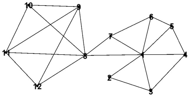
Although node 1 is connected to the most nodes in the network (nodes 2–8) it is not a “key player” in the network, because its removal does not disconnect the network. However, removal of node 8 (a “key player”) results in the network fracturing into two smaller components that are disconnected from each other. Adapted from Borgatti (2006).

The removal of nodes from a network in the negative key player problem sounds similar to the concept of a cut-edge or a cut-vertex in network analysis. In a cut-edge, a connection is removed in a network to partition the network. In a cut-vertex, a node (and the connections to and from it) is removed from the network. What again separates the negative key player problem from the similar concepts of cut-edges and cut-vertices is the ensemble issue described by Borgatti (2006). The set of nodes whose removal causes maximal partitioning of the network may differ from a list of nodes that simply lead to one part of the network being disconnected from another part of the network. Imagine if the connections to node 2 were removed from Figure 2. The removal of these connections would result in node 2 being isolated from nodes 1, and nodes 3–12. Preventing node 2 from communicating with the rest of the network could disrupt processing in the system. But such a “cut” is not likely to be as disruptive as the removal of nodes like node 8 from the system, whose removal prevents nodes 1–7 in the network from communicating with nodes 9–12 in the network. See Borgatti (2006) for a more extensive discussion of how key players differ from related concepts in network science.

Turning now to the cognitive domain, we wondered if an analogous set of words existed in the mental lexicon. That is, is there a set of “keywords” that play an important role in holding the lexical network together? If such words do indeed exist in the lexicon, how might they influence lexical processing? The existence of such words in the lexicon could provide new insight into various developmental or acquired language disorders. In individuals with acquired language disorders, including various types of aphasia, treatments that focus on the re-acquisition or rehabilitation of such keywords could facilitate language recovery. In individuals learning a (first or second) language, introducing keywords early in the process could accelerate (or otherwise facilitate) the acquisition of new words.

The psychological construct of “keywords” in the mental lexicon has wide-ranging and important implications with much practical value. However, before we can address the interesting extensions of this concept, we must first determine if such keywords even exist in the mental lexicon. To that end we used the algorithm developed by Borgatti (2006) to identify a small subset of nodes in the phonological network examined in Vitevitch (2008) that would lead to fracturing of the network (or, barring that, increasing the average distance between nodes) if they were removed.

Although there are certain psycholinguistic tasks that make it difficult to retrieve certain words, leading to the temporary “removal” of a word from the lexicon—such as the tip-of-the-tongue elicitation task (Brown & McNeill, 1966), or the verbal transformation task (Shoaf & Pitt, 2002)—we were uncertain of the consequences that even the temporary removal of keywords might have on lexical processing more generally, or in the long-term. Therefore, we opted for a method that would allow us to examine the influence of keywords on processing with a minimal potential for harm. To that end, we selected another set of words that were similar to the keywords in a variety of relevant lexical characteristics (e.g., word length, frequency of occurrence, number of phonological neighbors), but were not identified as being in crucial positions of the lexical network (i.e., they were not keywords). We then compared how participants responded to both sets of words in conventional psycholinguistic tasks. We reasoned that if keywords indeed played an important role in holding together the lexical network, then they should be responded to differently in terms of processing speed and/or accuracy than words that did not occupy such important positions in the lexical network. In what follows we report the results of three standard psycholinguistic tasks—perceptual identification, auditory naming, and auditory lexical decision—that used keywords and comparable non-keywords as stimuli.

Experiment 1a and 1b: Perceptual Identification Task

The present experiment used a conventional task in psycholinguistics, the perceptual identification task, to compare how keywords and words that resembled the keywords in numerous ways, but were not located in a crucial position in the lexical network (henceforth referred to as “foils”), were recognized. In the perceptual identification task, participants were asked to identify a stimulus word that was presented in a background of white noise. We then compared the accuracy of the responses to the keywords and the accuracy of the responses to the foils. This task was performed by a sample of undergraduate students (Experiment 1a) and replicated in a second sample from that population (Experiment 1b).

Methods

Participants

Twenty-five undergraduates enrolled in lower level psychology courses at the University of Kansas participated for partial course credit. All participants reported normal hearing and spoke English as their first language. A second sample of twenty-five participants was selected from the same population to replicate the result observed in the first sample.

Materials

A total of 50 words were used in the perceptual identification experiment: 25 keywords and 25 foils. A male native speaker of American English (the first author) produced all of the stimuli by speaking at a normal speaking rate and loudness in an IAC sound attenuated booth into a high-quality microphone, and recorded digitally at a sampling rate of 44.1 kHz with a Marantz PMD671 Portable Solid State Recorder. The pronunciation of each word was verified for correctness. Each stimulus word was edited using SoundEdit 16 (Macromedia, Inc.) into an individual sound file. The amplitude of the individual sound files was increased to their maximum without distorting the sound or changing the pitch of the words by using the Normalization function in SoundEdit 16. The same program was used to degrade the stimuli by adding white noise equal in duration to the sound file. The white noise was 15 dB less in amplitude than the mean amplitude of the sound files. Thus, the resulting stimuli were presented at a +15 dB signal to noise ratio (S/N).

The 25 key words were selected using the fragmentation measure described in Borgatti (2006; and also described in Appendix A) and implemented in the Keyplayer 1.44 software (Borgatti, 2008). Ideally, items in the set selected by the algorithm result in the connected network fracturing into several smaller components when they are removed. If it is not possible to create separate components, then items are selected whose removal increases the average distance among nodes in the network.

To assess how well the selected set fractures the network, a measure known as fragmentation is used. Fragmentation, F, is defined as the ratio between the number of pairs of nodes that are not connected once the set of key players have been removed, and the total number of pairs in the original fully connected network (i.e., prior to the removal of the set of key players). The minimum fragmentation value of 0 indicates the network consists of a single component (i.e., it has not fractured, but average distances have increased), and the maximum fragmentation value of 1 indicates the network has been completely fractured, solely consisting of isolates, or nodes with no connections (i.e., every node is unreachable). The set of 25 keywords (listed in Appendix B) that were selected from the 6,508 words in the giant component of the network examined by Vitevitch (2008) had a fragmentation score of .125, breaking it into 29 components (including 6 isolates, 22 components ranging in size from 2–63 nodes, and one large component that contained 6,060 of the 6,508 words from the initial giant component).

Borgatti (2006) notes that high fragmentation values will typically occur when the graph is not very cohesive. The giant component of the phonological network is very cohesive (as indicated by the relatively high average values of clustering coefficient, the average shortest path length, transitivity, ratio of edges to vertices in the giant component, and the amount of assortative mixing by degree reported in Arbesman et al., 2010). Given the high cohesiveness of the phonological network, the relatively low fragmentation value obtain in the present analysis is not surprising.

For further comparison, Borgatti (2006) found in the giant component of 63 suspected terrorists (the entire network contained 74 suspected terrorists; Krebs, 2002) a fragmentation score of .59, with the giant component fracturing into 7 smaller components when three key players were removed. In a network of advice-seeking in a consulting company (Cross, Parker & Borgatti, 2002), Borgatti (2006) found that the component with the strongest ties (containing 32 individuals) had a fragmentation score of .817 when two nodes were removed, and broke into four components (including one isolate). In the same network, he observed a fragmentation score of .843 when three nodes were removed from the network, breaking it into six components (including three isolates).

Although the fragmentation scores of the two networks examined by Borgatti (2006) were much higher than the fragmentation score observed in the present network, the networks examined by Borgatti (2006) were much smaller than the network used in the present study. Furthermore, the sets obtained by Borgatti (2006) contained significantly fewer key players than the set obtained in the present study. We selected 25 keywords in the present study because our previous experience suggested that 25 items was the smallest number of words per condition that we could use in a psycholinguistic experiment, and because attempts to obtain a set containing more than 25 key players from our network resulted in significant increases in computer processing time to obtain the set of keywords, but less optimal fragmentation scores than those obtained from the set containing 25 key players. Given the lower fragmentation scores for a larger set of keywords, we decided to use the smaller set of 25 words with the higher fragmentation score.

It is important to note that the fragmentation score describes the extent to which the set of key players fragments the network. It is not an average of the individual items in the set. In other words, individual items in the set do not have individual fragmentation scores. Furthermore, because the fragmentation score describes the extent to which the set of key players fragments the network it cannot be calculated for items that are not key players (i.e., for items that are not removed from the network). In other words, a fragmentation score for the set of foil words does not exist; such a value is undefined.

The keywords and foils were comparable on a number of other measures, including word length (measured in number of phonemes, and in number of syllables), frequency of occurrence, subjective familiarity, phonological neighborhood density (known as degree in a network of phonological word-forms), neighborhood frequency, phonotactic probability, and spoken duration. We also matched the keywords and foils on a number of network measures as well. The value of each measure for each word is listed in Appendix B, along with the words in each condition. Because of the strict matching of keywords and foils, paired t-tests were used to compare the lexical characteristics of words in the two groups.

Word length

Word length was measured in number of phonemes per word and in number of syllables per word. The keywords had a mean of 4.36 (SD = .76) phonemes per word and the foils had a mean of 4.52 (SD = .71) phonemes per word; the difference in number of phoneme per words was not statistically significant (t (24) = .89, p = .38). The two sets of words were also comparable when word length was measured in number of syllables per word. The keywords had a mean of 1.72 (SD = .54) syllables per word and the foils had a mean of 1.68 (SD = .48) syllables per word; the difference in number of syllables per words was not statistically significant (t (24) = .33, p = .75).

Subjective familiarity

Subjective familiarity was measured on a seven-point scale (Nusbaum, et al., 1984). The rating scale ranged from 1, You have never seen the word before to 4, You recognize the word, but don’t know the meaning, to 7, You recognize the word and are confident that you know the meaning of the word. Keywords had a mean familiarity value of 5.84 (SD = 1.65) and foils had a mean familiarity value of 5.63 (SD = .015, t (24) = .51, p = .61). Given that a rating of 6 in the Nusbaum et al. norms (1984) indicated that You think you know the meaning of the word, but are not certain that the meaning you know is correct, the mean familiarity value for the words in the two groups indicates that participants were likely to recognize most of the items as real word even though they might not know the meaning of a particular word.

Word frequency

Word frequency refers to how often a word in the language is used. When data, such as word-frequency counts, exhibit a skewed distribution, a standard statistical practice is to transform the data to better approximate a normal distribution (Tabachnick & Fidell, 2012); hence our use of log-base 10 of the raw frequency values in the present analyses. Average log word frequency (log-base 10 of the raw values from Kučera & Francis, 1967) was .82 (SD = .85) for the keywords, and .67 (SD = .76) for the foils (t (24) = .69, p = .49).

We also computed word frequency using the word frequency norms of Brysbaert and New (2009). Note that one word, inurn, was not found in the Brysbaert and New norms, so we substituted the frequency value (.02) of the related word inurnment. To make these values comparable to the Kučera & Francis norms we took the counts per million from the Brysbaert and New norms (SUBTL_WF) added 1 to those values and then took the log₁₀ of those values. The mean word frequency was .81 (SD =.83) for the keywords, and .64 (SD = .69) for the foils (t (24) = .79, p = .43). As these analyses show, regardless of the norms used to assess word frequency, the foils and keywords are relatively well matched with regards to frequency of occurrence.

Neighborhood density

Neighborhood density was defined as the number of words that were similar to a target word. Similarity was assessed with a simple and commonly employed metric (Greenberg & Jenkins, 1967; Landauer & Streeter, 1973; Luce & Pisoni, 1998; see also Otake & Cutler, 2013). A word was considered a neighbor of a target word if a single phoneme could be substituted, deleted, or added into any position of the target word to form that word. For example, the word cat has phonological neighbor words like _at, scat, mat, cut, cap. Note that cat has other neighbors, but only a few were listed for illustration. The mean neighborhood density of the keywords was 6.88 neighbors (SD = 4.43) and the mean neighborhood density of the foils was 6.56 neighbors (SD = 6.31; (t (24) = .31, p = .76).

Neighborhood frequency

Neighborhood frequency is the mean word frequency of the neighbors of the target word. Keywords had a mean log neighborhood frequency value of 1.28 (SD = .54), and foils had a mean log neighborhood frequency value of 1.18 (SD = .77, t (24) = .68, p = .50).

Phonotactic probability

The phonotactic probability was measured by how often a certain segment occurs in a certain position in a word (positional segment frequency) and by the segment-to-segment co-occurrence probability (biphone frequency; Vitevitch & Luce, 1998; 2005). The mean positional segment frequency (summed across positions) for keywords was .226 (SD = .098) and for foils was .236 (SD = .091, t (24) = .52, p = .61). The mean biphone frequency (summed across positions) for keywords was .022 (SD = .01) and .021 (SD = .02, t (24) = .58, p = .56). These values were obtained from the web-based calculator described in Vitevitch and Luce (2004).

Duration

The duration of the stimulus sound files was equivalent between the two groups of words. The mean overall duration of the keywords was 625.08 ms (SD = 87.47) and 624.32 ms (SD = 75.55) for the foils (t (24) = .03, p = .98).

Clustering Coefficient

Clustering coefficient, C, is a micro-level network metric that measures the extent to which the neighbors of a given node are also neighbors of each other. C was computed for each word (i.e., the local clustering coefficient for an undirected graph) as in previous studies (e.g., Chan & Vitevitch, 2009; Chan & Vitevitch, 2010; Vitevitch, Chan & Roodenrys, 2012) using equation (1):

$$C_i=\frac{2\left|\{e_{jk}\}\right|}{k_i(k_i-1)}$$ (Eq. 1)

e_jk refers to the presence of a connection (or edge) between two neighbors (j and k) of node i, |…| is used to indicate cardinality, or the number of elements in the set (not absolute value), and k_i refers to the degree (i.e., neighborhood density) of node i. By convention, a node with degree of 0 or 1 (which results in division by 0—an undefined value) is assigned a clustering coefficient value of 0. Note that degree > 1 for all of the words used in the present studies. Thus, the (local) clustering coefficient is the proportion of connections that exist among the neighbors of a given node divided by the number of connections that could exist among the neighbors of a given node. The mean value of C for the keywords was .23 (SD = .11) and the mean value of C for the foils was .21 (SD = .24; (t (24) = .49, p = .62).

Closeness Centrality

Given the influence of closeness centrality that Iyengar et al. (2012) found in the word-morph game we also controlled the closeness centrality of the foils and keywords. Closeness assesses how far away other nodes in the network are from a given node. See footnote 1 for a more precise definition of closeness centrality. A node with high closeness centrality is very close to many other nodes in the network, requiring that, on average, only a few links be traversed to reach another node. A node with low closeness centrality is, on average, far away from other nodes in the network, requiring the traversal of many links to reach another node. The mean value of closeness centrality for the keywords was .17 (SD = .02) and the mean value of closeness centrality for the foils was .16 (SD = .03; (t (24) = .72, p = .48), indicating that the keywords and the foils were, on average, about the same distance from all other nodes in the network. We report the inverse of the closeness centrality measures computed by Gephi (Bastian, Heymann & Jacomy, 2009), which is the more common way of reporting closeness centrality measures (and corresponds to the formula we provided in Footnote 1).

Community structure

The foils and keywords used in the present study came from the giant component of the phonological network examined in Vitevitch (2008). Recently, Siew (2013) examined the community structure of words in the giant component of that network. Community structure refers to the presence of densely connected groups within a larger network; items within a community tend to be more similar to (and more connected to) items in the same community than to items in other communities. In the present case, we examined which communities in the giant component the keywords and foils resided in. We found that 80% of the foil words resided in the same community as a keyword. The large amount of overlap in the communities that the foils and keywords reside in further indicates how similar the foils and keywords are to each other.

Procedure

Participants were tested individually. Each participant was seated in front of an iMac computer running PsyScope 1.2.2 (Cohen et al., 1993), which controlled the presentation of stimuli and the collection of responses.

In each trial, the word “READY” appeared on the computer screen for 500 ms. Participants then heard one of the randomly selected stimulus words imbedded in white noise through a set of Beyerdynamic DT 100 headphones at a comfortable listening level. Each stimulus was presented only once. The participants were instructed to use the computer keyboard to enter their response (or their best guess) for each word they heard over the headphones. They were instructed to type “?” if they were absolutely unable to identify the word. The participants could use as much time as they needed to respond. Participants were able to see their responses on the computer screen when they were typing and could make corrections to their responses before they hit the RETURN key, which initiated the next trial. The experiment lasted about 15 minutes. Prior to the experiment, each participant received five practice trials to become familiar with the task. These practice trials were not included in the data analyses.

Results and Discussion

Given the way in which the foils and keywords were matched on a number of relevant variables, and the categorical rather than continuous nature of “keyword-ness” (i.e., a word either is or is not a keyword) the minimally sufficient analysis is, of course, a factorial ANOVA. However, the field of psycholinguistics still holds many beliefs (some of them erroneous, as described in Raaijmakers, Schrijnemakers & Gremmen, 1999) about the influence that variability in the stimuli (or “items”) have on observed effects. To address those beliefs we used multi-level modeling (Baayen, 2010), a technique that simultaneously assesses the influence of both “participant” and “item” variability, to analyze the present data. Specifically, a 2-level model was created for each analysis with participant as the level 2 unit and observations as the level 1 unit.

Accuracy rates (treated as a binomial variable) were the dependent variable of interest in a logistic linear mixed effects model using the statistical software R (R Development Core Team, 2013) with the package “lme4” (Bates, Maechler, & Bolker, 2012) with subject and item as crossed random effect factors, and a random slope and a random intercept. Condition (foil/keyword) was dummy coded (0/1). Thus, a positive coefficient estimate indicates responses to keywords were more likely to be correct compared to responses to foils.

A response was scored as correct if the phonological transcription of the response matched the phonological transcription of the stimulus. Misspelled words and typographical errors in the responses were scored as correct responses in certain conditions: (1) adjacent letters in the word were transposed, (2) the omission of a letter in a word was scored as a correct response only if the response did not form another English word, or (3) the addition of a single letter in the word was scored as a correct response if the letter was within one key of the target letter on the keyboard. Responses that did not meet the above criteria were scored as incorrect.

The results show a statistically significant difference in the accuracy rate of the keywords and foils, such that keywords were responded to more accurately (mean = 54.72%; SD = 1.99) than were the foils (mean = 48.0%; SD = 2.63). We replicated the experiment with another sample of twenty-five participants drawn from the same population, and observed in this second sample a statistically significant difference in the accuracy rate of the keywords and foils. In the second sample of participants keywords were also responded to more accurately (mean = 53.28%; SD = 2.69) than were the foils (mean = 47.36%; SD = 2.54).

The results from two samples of participants in Experiment 1 showed that the set of keywords were identified in noise more accurately than a set of foil words comparable to the keywords on several lexical characteristics known to affect lexical processing (e.g., word length, frequency of occurrence, neighborhood density, phonotactic probability, etc.) and several network science measures that have recently been shown to influence lexical processing (e.g., clustering coefficient and closeness centrality). This result is striking because widely accepted models of spoken word recognition (Gaskell & Marslen-Wilson, 1997; Luce & Pisoni, 1998; Marslen-Wilson, 1987; McClelland & Elman, 1986; Norris, 1994), which account for the influence of many of these lexical characteristics, would predict no difference in how these two sets of words are responded to.

Recall that keywords occupy unique positions in the lexical network, such that they keep a network from fracturing into smaller components and help to minimize the shortest average distance among nodes in the network. Despite being very similar to another set of words (i.e., the foils) drawn from the lexicon, the keywords were identified more accurately than the other set of comparable words. The present result demonstrates the importance of understanding how the structural organization of phonological word-forms in the lexicon can influence language processing.

The present result also illustrates how a network concept from one domain can be used to explore another, seemingly disparate domain. Just as key players in a social network occupy important positions in the system that allow them to influence how information (or diseases) spread across a population of people, keywords in the lexical network occupy unique positions in the mental lexicon. The position of such words in the lexical network affords them privileged access during spoken word recognition. To further examine the privileged access of keywords compared to words that are—on the surface—quite comparable, we used two more conventional psycholinguistic tasks to assess how processing times might be affected by network location. These tasks, the auditory naming task and the auditory lexical decision task, again allowed us to investigate the concept of keywords in the mental lexicon without the potential risks that might accompany other tasks—such as the tip-of-the-tongue elicitation task or the verbal transformation illusion—that temporarily “remove” a word from the lexicon.

Experiment 2: Auditory Naming Task

In the auditory naming task, participants hear a spoken stimulus and must repeat it as quickly and accurately as possible. In this case we compared how quickly and accurately participants responded to keywords and foils.

Methods

Participants

Twenty-five undergraduates enrolled in lower level psychology courses at the University of Kansas participated for partial course credit. All participants reported normal hearing and spoke English as their first language.

Materials

The same stimuli used in Experiments 1a and 1b were used in the present study, with the exception that the words were now presented without noise.

Procedure

The same equipment used in Experiments 1a and 1b was used in the present study. In the present experiment a headphone-mounted microphone (Beyerdynamic DT-109 headphones) was interfaced to the PsyScope button box to act as a response switch.

Participants saw the word READY flash on the screen to signal the start of a trial. A randomly selected stimulus was then played through the headphones. As soon as the participant spoke their response, the next trial began. Reaction time was measured from stimuli onset to the onset of the participant’s vocal response. Participant responses were also recorded and later analyzed for accuracy.

Results and Discussion

Multi-level modeling (Baayen, 2010) was again used with the same software and approach as that used in Experiment 1. Response time was the dependent variable of interest with subject and item as crossed random effect factors, and a random slope and a random intercept. Condition (foil/keyword) was dummy coded (0/1). Thus, a negative coefficient estimate indicates keywords had faster reaction times than foils. Only correct responses within 2 standard deviations of the mean response time were used in the analyses (resulting in 5.9% of the responses being excluded). The analysis showed that keywords (M = 977ms, SD = 88) were responded to significantly more quickly than foils (M = 995ms, SD = 88), indicting that keywords also have an advantage in processing speed over the foils in addition to the accuracy advantage observed in Experiment 1.

Experiment 3: Auditory Lexical Decision Task

Experiments 1 and 2 provided evidence to support the hypothesis that keywords do exist in the mental lexicon, and that they influence the speed and accuracy with which spoken words are recognized. We performed another experiment to bolster this empirical foundation. The purpose of the present experiment was to further examine keywords in the mental lexicon by employing another task that emphasizes the activation of lexical representations in memory—the auditory lexical decision task. Although the degraded stimuli in the auditory perceptual identification task (Experiment 1) is somewhat akin to the input we normally get in the real world (i.e., a signal produced by an interlocutor amidst a background of environmental sounds), it is important to further demonstrate that the effects observed in the auditory naming task (Experiment 2) generalize to stimuli that are not degraded in any way. The use of stimuli that are not degraded would also minimize the possibility that participants responded to the stimuli using some sort of sophisticated guessing strategy, which might occur in tasks using degraded stimuli (Hasher & Zacks, 1984).

The auditory lexical decision task has proven quite useful in examining the influence of many variables—including phonological neighborhood density, phonotactic probability, and neighborhood frequency—on spoken word processing (e.g., Luce & Pisoni, 1998; Vitevitch & Luce, 1999). In this task, participants are presented with either a word or a nonword (without any white noise) over a set of headphones. Participants are asked to decide as quickly and as accurately as possible whether the given stimulus is a real word in English or a nonsense word. In addition to using stimuli that are not degraded, the lexical decision task, like the auditory naming task used in Experiment 2, allows reaction time data to be assessed. Reaction times provide us with a means for investigating the time course of spoken word recognition. Based on the results of Experiment 2, we predicted that keywords would be responded to more quickly than the foils.

Method

Participants

Twenty-three undergraduates enrolled in lower level psychology courses at the University of Kansas participated for partial course credit. All participants reported normal hearing and English as their first language. All participants were also right-hand dominant.

Materials

The real words used in the present experiment were the 25 keywords and 25 foils that were used in the previous experiments. A total of 50 nonword stimuli were selected from Vitevitch and Luce (1999). All nonword stimuli were bisyllabic and are listed in Appendix C.

Procedure

The same equipment that was used in the previous experiments was used in the present experiment. In each trial, the word “READY” appeared on the computer screen for 500 ms. Participants then heard one of the randomly selected words or nonwords through a set of headphones at a comfortable listening level. Each stimulus was presented only once. The participants were instructed to respond as quickly and as accurately as possible whether the item they heard was a real English word or a nonword. If the item was a word, they were to press the button labeled ‘WORD’ with their right (dominant) hand. If the item was not a word, they were to press the button labeled ‘NONWORD’ with their left hand. Reaction times were measured from the onset of the stimulus to the onset of the button press response. After the participant pressed a response button, the next trial began. The experiment lasted about 20 minutes. Prior to the experimental trials, each participant received ten practice trials to become familiar with the task. These practice trials were not included in the data analyses.

Results and Discussion

Multi-level modeling (Baayen, 2010) was again used with the same software and approach as that used in Experiment 1. Response time was the dependent variable of interest with subject and item as crossed random effect factors, and a random slope and a random intercept. Condition (foil/keyword) was dummy coded (0/1). Again, a negative coefficient estimate indicates faster reaction times for keywords compared to foils. Only correct responses within 2 standard deviations of the mean response time were used in the analyses (resulting in 2.6% of the responses being excluded). The analysis showed that keywords (M = 896ms, SD = 77) were responded to significantly more quickly than foils (M = 928ms, SD = 94), further indicting that keywords also have an advantage in processing speed over the foils in addition to the accuracy advantage observed in Experiment 1. The results of this experiment also demonstrate that keywords do exist in the lexicon, and influence processes associated with spoken word recognition.

MegaStudy Analysis: Data from the English Lexicon Project

To further examine processing differences between the keywords and foils we analyzed the visual naming and visual lexical decision data from the English Lexicon Project (ELP; Balota et al. 2007). The ELP is a large database of descriptive data (e.g., word frequency, number of orthographic and phonological neighbors, etc.) for over 40,000 words. The database also contains behavioral data from 1,260 participants across 6 different universities who responded to those words in a visual naming task and a visual lexical decision task. Balota et al. (2007; page 457) suggested that, “…these data will be important for researchers interested in targeting particular variables. In some cases, experiments might be replaced by accessing the database.” Rather than conduct yet another experiment to demonstrate that keywords in the lexicon influence processing, we analyzed the behavioral data in the ELP for our keywords and foils.

We recognize that the nonwords that appeared in our auditory lexical decision task differed from those used in the ELP, which could lead to differences in how the real words are responded to (see Vitevitch (2003) and Vitevitch & Donoso (2011) for ways in which the nonwords that are used in an auditory lexical decision task can influence processing of the real word targets, and Andrews (1997) for a review of such effects in visual lexical decision tasks). Despite that difference we think it is still valuable to examine independently collected data for possible influences of keywords on processing.

Another difference between the ELP and the present studies is that the stimuli in the ELP were presented visually rather than auditorily as in the present experiments. Given the results of Yates (2013), we believe there is good reason to explore how phonological characteristics might influence the visual domain. Yates (2013) found that words that differed in the phonological clustering coefficient (as measured in the network analyzed in Vitevitch, 2008) were responded to in the same way as observed in Chan and Vitevitch (2009)—words with low clustering coefficient were responded to more quickly than words with high clustering coefficient—even though Yates presented the stimuli visually to participants in a lexical decision task instead of auditorily as in Chan and Vitevitch (2009).

The final difference that we wish to highlight is in the statistical analyses we used to examine the ELP data and the statistical analyses we used in the experiments in the present study. To examine the ELP data we used a between groups items analysis, an analysis that is minimally sufficient and the only analysis that can be performed on the available data. This difference in the type of analyses used is relevant because it is well-known that between groups analyses have less statistical power than some other types of analyses.

Keeping in mind these differences between the experiments in the present study and the ELP data, we examined the visual naming data in the ELP and found that keywords (M = 649ms, SD = 65) tended to be responded to more quickly than foils (M = 667ms, SD = 73; t (43) = .86, p = .39). (Note that the following words from the present study were not in the ELP database: auricle, feudal, inurn, leva, and ling.) Furthermore keywords (M = 95%, SD = 10) tended to be responded to more accurately than foils (M = 91%, SD = 13; t (43) = 1.18, p = .24). The differences in naming time and naming accuracy are, of course, not statistically significant by conventional standards, but it is noteworthy that the difference in naming time was in the same direction (and comparable in magnitude) as the difference observed in the auditory naming task reported in the present study.

For the visual lexical decision data in the ELP we found that keywords (M = 682ms, SD = 98) tended to be responded to more quickly than foils (M = 712ms, SD = 135; t (42) = .83, p = .41), and that keywords (M = 87%, SD = 20) tended to be responded to more accurately than foils (M = 78%, SD = 25; t (42) = 1.26, p = .21). As with the ELP visual naming data, the difference in the ELP visual lexical decision data does not reach statistical significance by current conventions. However, it is striking that for the same set of words the differences in response time in both the visual naming and lexical decision data from the ELP were in the same direction and comparable in magnitude to the results observed in the present experiments.

To further examine the influence of keywords on lexical processing we followed another suggestion of Balota et al. (2007; page 457), “…one can resample different sets of items with particular characteristics from the database.” It is, of course, not possible to find other words that form the optimal set of 25 key players in the lexicon, so in the present case we sampled another set of foil words that were again comparable to the keywords on a variety of lexical and network characteristics (the words and characteristics are listed in Appendix D).

In the visual naming data in the ELP we found that keywords (M = 649ms, SD = 65) tended to be responded to more quickly than the second set of foils (M = 683ms, SD = 86; t (42) = 1.48, p = .15). Furthermore, keywords (M = 95%, SD = 9) tended to be responded to more accurately than the second set of foils (M = 94%, SD = 13; t (42) = .48, p = .63). For the visual lexical decision data in the ELP we found that keywords (M = 682ms, SD = 98) tended to be responded to more quickly than the second set of foils (M = 690ms, SD = 79; t (42) = .32, p = .75), and that keywords (M = 87%, SD = 20) tended to be responded to more accurately than the second set of foils (M = 81%, SD = 24; t (42) = .85, p = .40). Despite the failure of the ELP analyses of an additional set of foils to reach statistical significance by current conventions, we were again struck by the fact that the differences in both the visual naming and lexical decision data from the ELP were in the same direction and comparable in magnitude to the results observed in the present experiments.

One possible interpretation of the ELP results is that network science measures may reflect more central aspects of lexical processing for both orthography and phonology. Alternatively, as Yates (2013) suggests, such results may indicate that phonology influences visual word recognition. We prefer a more cautious interpretation of the ELP data; the trends observed in the present analyses simply provide additional and converging evidence that keywords in the mental lexicon influence lexical processing.

General Discussion

In three conventional psycholinguistic tasks and four additional analyses of data from the English Lexicon Project (ELP) we found a processing advantage for keywords relative to foils. Recall that keywords occupy a unique position in the lexical network, holding together several smaller components in the network, and minimizing the overall distance between nodes in the network. We selected as foils words that did not occupy such positions in the lexical network, but were comparable to the keywords on a number of relevant lexical characteristics, including frequency of occurrence, neighborhood density (i.e., degree), word length, phonotactic probability, and several relevant network science characteristics. Given the comparability of the keywords and foils on these lexical characteristics, widely accepted models of spoken word recognition (Gaskell & Marslen-Wilson, 1997; Luce & Pisoni, 1998; Marslen-Wilson, 1987; McClelland & Elman, 1986; Norris, 1994), which account for the influence of these variables on processing, do not predict any difference in how quickly or accurately the keywords and foils should be responded to. However, statistically significant differences were observed, with keywords being responded to more quickly and accurately than the foils in several conventional psycholinguistic tasks.

The present finding adds to an increasing amount of evidence that suggests that the structure of the lexical network—as described in Vitevitch (2008) and Arbesman et al. (2010)— influences the speed and accuracy of various aspects of lexical processing (e.g., Chan & Vitevitch, 2009, 2010; Iyengar et al, 2012; Vitevitch et al., 2011; Vitevitch, Chan & Goldstein, 2013). It has been recognized for some time that the structure of the lexicon influences lexical processing. Consider this statement by Luce and Pisoni (1998; page 1): “…similarity relations among the sound patterns of spoken words represent one of the earliest stages at which the structural organization of the lexicon comes into play.” What has been missing until recently, however, is the right set of tools to measure the structure of the lexicon. Previous findings by Chan and Vitevitch (2009; 2010), Vitevitch (2008) and others, as well as the present findings illustrate how the methods and theoretical framework of network science can be used to measure other aspects of lexical structure—not just at the micro-level, but at the meso- and macro-level—and examine how that structure influences processing. The present findings also demonstrate how findings from one domain, such as key players in a social network, can help us to explore another, seemingly unrelated, domain, such as key words in a lexical network.

So, why are keywords responded to more quickly and accurately than comparable foils? We propose that indirect forces, such as the activation of nearby words—in addition to the direct activation of the keywords and foils themselves—strengthens the representations of keywords and foils. Even though the keywords and foils may not be directly activated, the activation of nearby neighbors will spread to and partially activate the keywords and foils, further strengthening those indirectly (or implicitly) activated items (Nelson, McKinney, Gee & Janczura, 1998). The location of the keywords at critical junctures in the network results in the lexical equivalent of an entrepreneurial “middle-man” receiving more of this indirect activation than the foils. The accumulation of this indirect activation over time may lower the activation threshold, or raise the resting activation level of keywords more than foils, enabling them to be retrieved more quickly and accurately than foils.

Widely accepted models of spoken word recognition all agree that several similar sounding competitors are partially activated during spoken word recognition, with the target word ultimately winning that competition and being recognized. These models, however, explicitly say little if anything about the long-term and cumulative effects of the repeated, partial activation of those losing competitors on the subsequent recognition of those spoken words. Work from other areas of Psychology, however, suggests that partial and indirect influences on subsequent processes are not implausible.

Consider first simulations described by Grossberg (1987) that examined how two uncommitted nodes in an adaptive resonance network (a different type of network than that examined in the present manuscript) compete to represent a novel input. Both nodes adjust their connection weights to represent the novel input, but ultimately one node better represents the input than the other and becomes committed to represent that information. The “losing” node, however, in attempting to represent the novel input has configured its weights in such a way that it, rather than some other uncommitted node, can better represent the next new input if that new input is similar to the input from the previously lost competition. In other words, the partial activation of a node during previous, but unsuccessful, attempts to acquire new information can influence subsequent attempts to acquire new information. Grossberg’s (1987) work in adaptive resonance theory (ART) is one demonstration of how partial activation of a “competitor” can affect subsequent processing.

Another way in which partial activation of competitors can affect subsequent processing is observed in the phenomenon known as phonological false memories (Sommers & Lewis, (1999); see Roediger & McDermott (1995) for semantic false memories). In phonological false memories, words such as at, scat, mat, cut, and cap are presented to participants for study. In subsequent recall or recognition tasks, participants are likely to indicate that the word cat appeared in the study list, when in fact it did not (Sommers & Lewis, 1999; Vitevitch et al., 2012). Such findings further suggest that the partial and indirect activation of cat during the presentation of the words in the study list can influence subsequent recall and recognition processes.

Evidence that indirect and partial activation of lexical representations influences spoken word recognition also comes from Geer and Luce (2012). They found evidence in an auditory shadowing task and a lexical decision task that suggests that partially activated, indirect neighbors (i.e., words 2 connections away from the target in a lexical network) inhibit direct neighbors of a target word (i.e., words 1 connection away from the target), thereby reducing the amount of inhibition that the target word receives from those direct neighbors. Referring to Figure 1, if speech is the target word, the word spud would inhibit the word speed, the word beach would inhibit peach, etc., thereby reducing the amount of inhibition that speech receives from speed, peach, etc. Said another way, the words that inhibit a target word are themselves inhibited by other words. As shown by Geer and Luce (2012), the number of indirect neighbors can influence retrieval of a target word by moderating the influence that direct neighbors have on the target word (also see Vitevitch, Goldstein & Johnson (submitted) for additional evidence that indirect neighbors influence processing).

The influence of indirectly and partially activated representations on lexical retrieval has also been observed in patients with aphasia participating in a treatment technique known as Verb Network Strengthening Treatment (VNeST) developed by Edmonds, Nadeau and Kiran (2009, see also Semantic Feature Analysis; Coelho, McHugh & Boyle, 2000). VNeST attempts to improve sentence production in patients with aphasia by training patients to retrieve verbs, which partially activate related verbs as well as the patients and agents associated with the verbs. This approach has effectively promoted generalization from single word naming to connected speech in patients with moderate aphasia. These findings lend some credence to the hypothesis that indirect activation may differentially influence the subsequent accessibility of keywords and foils due to their location in the lexical network.

We acknowledge that this initial exploration of keywords in the phonological lexicon is tentative. However, we dared not “remove” such words from the lexicon—even temporarily via psycholinguistic tasks such as tip-of-the-tongue elicitation, or the verbal transformation illusion—in our initial exploration of this psychological construct, because of concern over potential long-term or wide-spread effects on lexical processing. Our findings clearly show that certain words occupy “key” positions in the lexical network, and that these “keywords” are processed more quickly and accurately than words that resemble them in many other ways. The present findings now open many avenues for future research in other domains of language, including language acquisition, understanding lexical processing in individuals affected by language disorders, and in the development of clinical or therapeutic applications.

Furthermore, network science offers a unique and powerful set of tools to measure the structure of complex systems at multiple scales: micro-, meso- and macro-level. Important discoveries in the domains of biology, technology, and social interaction have been made using the tools of this approach (for a brief review see Albert & Barabási, 2002; Brandes et al., 2013). As demonstrated in the present study, adopting this approach in the psychological sciences can lead to new discoveries (e.g., how the structure of the mental lexicon influences certain aspects of language processing), and to an expansion in the range of questions investigated by psychological scientists. Several other areas in psychology have benefitted from adopting the analytic tools of network science (Goldstone et al., 2008; Griffiths et al., 2007; Hills et al., 2009; Iyengar et al., 2012; Sporns, 2010; Steyvers & Tenenbaum, 2005). We urge more psychological scientists to consider how the network science approach might lead to new questions and novel insights.

Although we are enthusiastic about the potential insights that network science can provide various area of psychology, we would be remiss if we did not also note that networks are not suitable for all problems or research questions. Researchers who desire to use the theoretical framework and analytic tools of network science should think carefully about how well entities and relationships among those entities in a given domain map onto nodes and connections in a network representation (see Valente (2012) for a similar point regarding network interventions).

Furthermore, even if a problem is amenable to network analysis, not all network measures may be relevant in a given domain (Brandes et al., 2013). For example, there are many measures of centrality and “importance” in network analysis, but of those many measures, the negative-Key Player Problem (Borgatti, 2006) mapped reasonably well onto a linguistically relevant phenomenon, namely, the inability to retrieve a word from the lexicon, as one might experience temporarily in the tip-of-the-tongue phenomenon (see Borgatti (2005) for a discussion of which centrality measures are appropriate in various contexts). Given the demonstrable influence of “keyword-ness” on processing observed in the present study, this concept warrants further exploration in several other areas of language processing. There are likely other concepts from network science, perhaps even phenomena in social networks that might also “translate” to the cognitive domain, and warrant investigation. We hope that psychologists investigating those other domains will consider what the network science approach has to offer.

Table 1.

Coefficient of the accuracy rates in the foils and keywords, along with the estimate, standard error, z-value and p-value for Experiment 1a and 1b.

Experiment 1a
	Estimate	Standard Error	z-value	p-value
Intercept	−0.08076	0.08850	−0.91	0.3615
Foil/Keyword	0.27068	0.11462	2.361	0.0182

Experiment 1b
	Estimate	Standard Error	z-value	p-value
Intercept	−0.10570	0.08011	−1.319	0.1870
Foil/Keyword	0.23770	0.11660	2.038	0.0415

Table 2.

Coefficient of the difference in response times, along with the estimate, standard error, t-value and p-value for Experiment 2.

Experiment 2
	Estimate	Standard Error	t-value	p-value
Intercept	996.081	17.465	57.03	0.0000
Foil/Keyword	−20.88	7.068	−2.95	0.0031

Table 3.

Coefficient of the difference in response times, along with the estimate, standard error, t-value and p-value for Experiment 3.

Experiment 3
	Estimate	Standard Error	t-value	p-value
Intercept	931.46	17.15	54.30	0.0000
Foil/Keyword	−25.26	10.38	−2.43	0.0149

Highlights.

• Keywords are words that hold a lexical network together.

• Three psycholinguistic tasks examined responses to keywords and comparable foils.

• Keywords were responded to more quickly and accurately than the comparable words.

• The implications of keywords for normal processing are discussed.

• The implications for language disorder are also discussed.

Appendix A

The fragmentation measure (^DF) is derived in Borgatti (2006). The final form of the equation (listed as Equation (9) in Borgatti, 2006) is:

$${}^{D}F=1-\frac{2{\sum }_{i>j}\frac{1}{d_{ij}}}{n(n-1)}$$

in which d_ij is a measure of reachability that varies between 0 and 1 for a given pair of nodes (indexed by i and j), and n is the number of nodes in the network.

Appendix B

Lexical and network characteristics of keywords used in Experiments 1–3

Word	KFfreq	SUBTLfreg	FAM	Density	NHF	PPseg	PPbi	C	Close.Cent.
Amend	.30	0.24	7.0	8	1.93	0.16	0.01	0.25	0.16
Auricle	.00	0.01	5.1	3	1.12	0.20	0.02	0.33	0.15
Bring	2.20	2.52	7.0	8	3.06	0.18	0.02	0.25	0.18
Colic	.00	0.18	4.0	6	2.67	0.31	0.04	0.13	0.17
Defy	.85	0.61	5.9	4	2.36	0.18	0.02	0.17	0.16
Filing	1.28	0.74	7.0	3	2.17	0.22	0.02	0.33	0.16
Fish	1.54	1.93	7.0	13	2.54	0.15	0.01	0.31	0.20
Inurn	.00	0.01	2.6	5	1.30	0.17	0.04	0	0.13
Leva	.00	0.04	2.4	5	2.67	0.21	0.01	0.30	0.15
Ling	.00	1.21	2.8	21	2.88	0.14	0.01	0.23	0.22
Lion	1.23	1.21	7.0	5	2.79	0.12	0.01	0.30	0.18
Milling	1.26	0.11	5.8	6	2.43	0.29	0.03	0.40	0.14
Misty	.60	0.41	6.8	5	2.13	0.36	0.05	0.20	0.17
Opine	.00	0.05	2.5	3	3.05	0.09	0.00	0.33	0.19
Over	3.09	3.12	7.0	10	2.57	0.03	0.01	0.18	0.17
Packet	.48	0.55	7.0	5	2.24	0.34	0.03	0.10	0.17
Pallet	.00	0.15	6.1	5	2.27	0.40	0.03	0.10	0.13
Pocket	1.66	1.56	7.0	7	1.50	0.32	0.03	0.33	0.15
Polite	.85	1.17	7.0	3	1.52	0.29	0.01	0.33	0.16
Scrawl	.00	0.09	5.7	4	1.72	0.26	0.01	0	0.16
Spring	2.10	1.51	7.0	5	1.92	0.26	0.02	0.10	0.14
Tenet	.00	0.05	5.5	6	2.23	0.34	0.04	0.20	0.17
Tense	1.18	1.05	7.0	12	2.75	0.26	0.03	0.32	0.19
Void	1.00	0.71	6.9	4	2.85	0.06	0.00	0.33	0.17
Wrist	1.00	1.05	7.0	16	2.43	0.31	0.06	0.16	0.20

Notes: KF_freq = log₁₀ value of frequency of occurrence (per million) from the Kučera & Francis (1967) norms. SUBTL_freg = log₁₀ value of frequency of occurrence (per million) from the Brysbaert & New (2009) norms. FAM = Subjective familiarity ratings from Nusbaum et al. (1984). Density = phonological neighborhood density (a.k.a. degree), which is the number of words that sound like the target word (based on the addition, deletion or substitution of a phoneme; Luce & Pisoni, 1998). NHF = Mean frequency of occurrence of the phonological neighbors (known as neighborhood frequency). PP_seg = sum of the positional segment frequency (obtained from Vitevitch & Luce, 2004). PP_bi = sum of the segment-to-segment co-occurrence probability (biphone frequency; obtained from Vitevitch & Luce, 2004). C = local clustering coefficient (Watts & Strogatz, 1998). Close.Cent. = closeness centrality (see text and Footnote 1 for more explanation).

Lexical and network characteristics of foils used in Experiments 1–3

Word	KFfreq	SUBTLfreg	FAM	Density	NHF	PPseg	PPbi	C	Close.Cent.
Album	.78	1.05	7.0	1	1.00	0.21	0.01	0	0.13
Aloft	.48	0.24	6.4	1	1.30	0.18	0.01	0	0.15
Attest	.30	0.16	5.1	2	2.84	0.21	0.02	0	0.16
Brief	1.86	1.19	6.9	8	2.08	0.18	0.02	0.42	0.18
Cockney	.00	0.13	3.3	1	1.48	0.29	0.02	0	0.16
Downy	.00	0.15	5.9	4	3.35	0.20	0.01	0.50	0.18
Espy	.00	0.02	2.7	1	1.95	0.12	0.00	0	0.16
Firm	2.03	0.08	6.8	2	1.54	0.14	0.01	0	0.15
Fuedal	.78	1.56	6.8	13	2.13	0.12	0.00	0.32	0.20
Lave	.00	0.04	2.8	22	2.85	0.09	0.00	0.33	0.22
Lighten	.00	0.84	7.0	6	2.88	0.14	0.01	0.27	0.19
Manna	.00	0.16	2.4	6	3.35	0.31	0.03	0.40	0.19
Mystic	.48	0.39	6.8	4	1.40	0.41	0.07	0.17	0.13
Osprey	.00	0.01	2.6	2	1.70	0.14	0.01	1.00	0.13
Party	2.33	2.37	7.0	5	3.05	0.35	0.03	0.20	0.16
Pasty	.30	0.21	6.2	8	2.58	0.37	0.04	0.11	0.17
Pilot	1.64	1.44	7.0	2	1.40	0.35	0.02	0	0.12
Poster	.60	0.84	7.0	7	2.26	0.35	0.04	0.10	0.16
Rent	1.32	1.55	7.0	17	2.84	0.31	0.04	0.36	0.20
Rupee	.78	0.02	2.4	2	1.00	0.15	0.01	0	0.13
Squirt	.00	0.57	7.0	5	1.87	0.22	0.01	0.10	0.16
Stilt	.00	0.02	5.5	7	3.05	0.28	0.02	0.14	0.18
Test	2.08	1.93	7.0	18	2.77	0.29	0.04	0.37	0.19
Torrid	.30	0.19	5.4	1	1.00	0.21	0.01	0	0.07
Vest	.60	0.82	6.9	19	2.76	0.26	0.03	0.36	0.19

Appendix C

The high-high and high-low phonotactic probability nonwords (in IPA) from Vitevitch & Luce (1999) used in Experiment 3

High-High	High-Low
fʌlʧʌn	sʌvwʌʃ
mʌbsʌʃ	ɹʌlʧʌtʃ
tʌlsʌʒ	sʌdʃʌʧ
hʌsʒʌn	lʌnđʌz
dʌssʌz	pʌmwʌʤ
sʌgkʌk	bʌlđʌg
taɪsdaɪp	saɪvđaɪm
vaɪɹvaɪk	ʧaɪnnaɪđ
baɪsfaɪk	saɪpkaɪđ
ɹaɪɹmaɪd	saɪmđaɪp
haɪssaɪb	gaɪnʃaɪp
vaɪtʤaɪnd	paɪtʧaɪb
kisʧin	bisđiʧ
kikɹig	sivjiʤ
sigɵin	dikziʤ
fikkit	ninjiʧ
pimfis	hinziʧ
vinɹiz	biltʃiʃ
vetɹeb	nesʧeɵ
mebkeb	tesʃeɵ
sebmep	pepʤeg
geswes	lelʧeg
hessep	henʃeg
pebɹem	pemʤeʤ
dɝsmɝn	pɝdʃɝʧ

Appendix D

Lexical and network characteristics of a second set of foils used in the ELP analyses

Word	KFfreq	SUBTLfreg	FAM	Density	NHF	PPseg	PPbi	C	Close.Cent.
angle	1.71	1.20	7.00	10	0.88	0.07	0.00	0.47	0.13
attention	2.25	2.00	7.00	2	1.48	0.28	0.03	0.00	0.11
breadth	0.85	0.16	5.08	2	1.69	0.21	0.02	1.00	0.16
cordon	0.30	0.29	3.27	3	0.82	0.27	0.03	0.00	0.16
debase	0.00	0.05	4.83	1	0.30	0.24	0.02	0.00	0.13
filter	0.95	0.62	6.92	3	0.30	0.07	0.01	0.00	0.16
fix	1.15	1.94	7.00	10	1.55	0.25	0.02	0.16	0.18
incur	0.70	0.19	4.67	2	0.40	0.18	0.04	1.00	0.10
lido	0.00	0.22	2.75	2	0.74	0.12	0.01	0.00	0.18
lilt	0.00	0.09	4.42	14	1.39	0.29	0.02	0.42	0.20
listen	1.71	2.74	7.00	5	1.55	0.22	0.03	0.20	0.17
minnow	0.00	0.10	5.42	3	0.60	0.27	0.02	0.33	0.17
molten	0.48	0.33	5.73	1	0.30	0.28	0.02	0.00	0.16
ochre	0.30	Not found	2.25	9	2.16	0.05	0.00	0.25	0.18
oral	1.43	0.73	7.00	8	2.72	0.10	0.00	0.14	0.18
palace	1.58	1.31	7.00	7	0.46	0.37	0.03	0.48	0.13
pander	0.00	0.05	4.92	7	0.23	0.34	0.04	0.19	0.15
platter	0.30	0.59	7.00	10	1.21	0.29	0.02	0.16	0.17
poodle	0.30	0.58	7.00	7	0.30	0.17	0.00	0.43	0.17
scotch	0.70	1.20	6.50	4	0.89	0.16	0.01	0.50	0.17
spree	0.60	0.50	6.08	5	1.18	0.24	0.02	0.20	0.15
tempo	0.60	0.43	6.08	3	1.26	0.22	0.02	1.00	0.12
term	1.90	1.27	7.00	13	2.20	0.12	0.00	0.31	0.21
vogue	5.00	0.52	6.50	4	1.42	0.09	0.00	0.17	0.19
wraith	0.00	0.08	4.42	15	1.65	0.09	0.00	0.55	0.21

Notes: KF_freq = log₁₀ value of frequency of occurrence (per million) from the Kučera & Francis (1967) norms. SUBTL_freg = log₁₀ value of frequency of occurrence (per million) from the Brysbaert & New (2009) norms. FAM = Subjective familiarity ratings from Nusbaum et al. (1984). Density = phonological neighborhood density (a.k.a. degree), which is the number of words that sound like the target word (based on the addition, deletion or substitution of a phoneme; Luce & Pisoni, 1998). NHF = Mean frequency of occurrence of the phonological neighbors (known as neighborhood frequency). PP_seg = sum of the positional segment frequency (obtained from Vitevitch & Luce, 2004). PP_bi = sum of the segment-to-segment co-occurrence probability (biphone frequency; obtained from Vitevitch & Luce, 2004). C = local clustering coefficient (Watts & Strogatz, 1998). Close.Cent. = closeness centrality (see text and Footnote 1 for more explanation).

References

- Albert R, Barabási AL. Statistical mechanics of complex networks. Review of Modern Physics. 2002;74:47–97. [Google Scholar]
- Amaral LAN, Scala A, Barthélémy M, Stanley HE. Classes of small-world networks. Proceedings of the National Academy of Sciences. 2000;97:11149–11152. doi: 10.1073/pnas.200327197. [DOI] [PMC free article] [PubMed] [Google Scholar]
- Andrews S. The effect of orthographic similarity on lexical retrieval: Resolving neighborhood conflicts. Psychonomic Bulletin & Review. 1997;4:439–461. [Google Scholar]
- Arbesman S, Strogatz SH, Vitevitch MS. The Structure of Phonological Networks Across Multiple Languages. International Journal of Bifurcation and Chaos. 2010;20:679–685. [Google Scholar]
- Baayen RH. A real experiment is a factorial experiment? The Mental Lexicon. 2010;5:149–157. [Google Scholar]
- Balota DA, Yap MJ, Cortese MJ, Hutchison KA, Kessler B, Loftis B, Neely JH, Nelson DL, Simpson GB, Treiman R. The English Lexicon Project. Behavior Research Methods. 2007;39:445–459. doi: 10.3758/bf03193014. [DOI] [PubMed] [Google Scholar]
- Barabási AL. Scale-Free Networks: A Decade and Beyond. Science. 2009;325:412–413. doi: 10.1126/science.1173299. [DOI] [PubMed] [Google Scholar]
- Bastian M, Heymann S, Jacomy M. Gephi: an open source software for exploring and manipulating networks. International AAAI Conference on Weblogs and Social Media.2009. [Google Scholar]
- Bates D, Maechler M, Bolker B. lme4: Linear mixed-effects models using S4 classes. R package version 0.999999-0. 2012 http://CRAN.R-project.org/package=lme4.
- Boccaletti S, Latora V, Moreno Y, Chavez M, Hwang D. Complex networks: structure and dynamics. Physics Reports. 2006;424:175–308. [Google Scholar]
- Borgatti SP. Centrality and network flow. Social Networks. 2005;27:55–71. [Google Scholar]
- Borgatti SP. Identifying sets of key players in a network. Computational, Mathematical and Organizational Theory. 2006;12:21–34. [Google Scholar]
- Borgatti SP. Keyplayer 1.44. [Computer software] Lexington, KY: Analytic Technologies; 2008. Retrieved from http://www.analytictech.com/keyplayer/keyplayer.htm. [Google Scholar]
- Brandes U, Robins G, McCranie A, Wasserman S. Editorial: What is network science? Network Science. 2013;1:1–15. [Google Scholar]
- Brown R, McNeill D. The “tip of the tongue” phenomenon. Journal of Verbal Learning and Verbal Behavior. 1966;5:325–337. [Google Scholar]
- Brysbaert M, New B. Moving beyond Kucera and Francis: A Critical Evaluation of Current Word Frequency Norms and the Introduction of a New and Improved Word Frequency Measure for American English. Behavior Research Methods. 2009;41:977–990. doi: 10.3758/BRM.41.4.977. [DOI] [PubMed] [Google Scholar]
- Burt R. Structural Holes and Good Ideas. American Journal of Sociology. 2004;110:349–399. [Google Scholar]
- Chan KY, Vitevitch MS. The influence of the phonological neighborhood clustering-coefficient on spoken word recognition. Journal of Experimental Psychology: Human Perception and Performance. 2009;35:1934–1949. doi: 10.1037/a0016902. [DOI] [PMC free article] [PubMed] [Google Scholar]
- Chan KY, Vitevitch MS. Network structure influences speech production. Cognitive Science. 2010;34:685–697. doi: 10.1111/j.1551-6709.2010.01100.x. [DOI] [PubMed] [Google Scholar]
- Charles-Luce J, Luce PA. Similarity neighborhoods of words in young children’s lexicons. Journal of Child Language. 1990;17:205–215. doi: 10.1017/s0305000900013180. [DOI] [PubMed] [Google Scholar]
- Coelho CA, McHugh RE, Boyle M. Semantic feature analysis as a treatment for aphasic dysnomia: A replication. Aphasiology. 2000;14:133–142. [Google Scholar]
- Cohen JD, MacWhinney B, Flatt M, Provost J. PsyScope: A new graphic interactive environment for designing psychology experiments. Behavioral Research Methods, Instruments, and Computers. 1993;25:257–271. [Google Scholar]
- Collins AM, Loftus EF. A spreading-activation theory of semantic processing. Psychological Review. 1975;82:407–428. [Google Scholar]
- Cramer AOJ, Waldorp LJ, van der Maas H, Borsboom D. Comorbidity: A network perspective. Behavioral and Brain Sciences. 2010;33:137–193. doi: 10.1017/S0140525X09991567. [DOI] [PubMed] [Google Scholar]
- Cross R, Parker A, Borgatti SP. Making Invisible Work Visible: Using Social Network Analysis to Support Strategic Collaboration. California Management Review. 2002;44:25–46. [Google Scholar]
- Edmonds LA, Nadeau SE, Kiran S. Effect of Verb Network Strengthening Treatment (VNeST) on lexical retrieval of content words in sentences in persons with aphasia. Aphasiology. 2009;23:402–424. doi: 10.1080/02687030802291339. [DOI] [PMC free article] [PubMed] [Google Scholar]
- Gaskell MG, Marslen-Wilson WD. Integrating form and meaning: A distributed model of speech perception. Language and Cognitive Processes. 1997;12:613–656. [Google Scholar]
- Geer M, Luce PA. Neighbors of Neighbors in Spoken Word Processing. 2012. Unpublished manuscript submitted for publication. [Google Scholar]
- Greenberg JH, Jenkins JJ. Studies in the psychological correlates of the sound system of American English. In: Jakobovits LA, Miron MS, editors. Readings in the psychology of language. Englewood Cliffs, N.J: Prentice-Hall; 1967. pp. xipp. 636pp. 186–200. [Google Scholar]
- Goldstone RL, Roberts ME, Gureckis TM. Emergent processes in group behavior. Current Directions in Psychological Science. 2008;17:10–15. [Google Scholar]
- Griffiths TL, Steyvers M, Firl A. Google and the mind: Predicting fluency with PageRank. Psychological Science. 2007;18:1069–1076. doi: 10.1111/j.1467-9280.2007.02027.x. [DOI] [PubMed] [Google Scholar]
- Grossberg S. Competitive learning: From interactive activation to adaptive resonance. Cognitive Science. 1987;11:23–63. [Google Scholar]
- Hasher L, Zacks RT. Automatic processing of fundamental information: The case of frequency of occurrence. American Psychologist. 1984;39:1372–1388. doi: 10.1037//0003-066x.39.12.1372. [DOI] [PubMed] [Google Scholar]
- Hills TT, Maouene M, Maouene J, Sheya A, Smith L. Categorical structure among shared features in networks of early-learned nouns. Cognition. 2009;112:381–396. doi: 10.1016/j.cognition.2009.06.002. [DOI] [PMC free article] [PubMed] [Google Scholar]
- Iyengar SRS, Madhavan CEV, Zweig KA, Natarajan A. Understanding Human Navigation Using Network Analysis. Topics in Cognitive Science. 2012;4:121–134. doi: 10.1111/j.1756-8765.2011.01178.x. [DOI] [PubMed] [Google Scholar]
- Kučera H, Francis WN. Computational Analysis of Present Day American English. Brown University Press; Providence: 1967. [Google Scholar]
- Krebs V. Uncloaking terrorist networks. First Monday. 2002;7(4) http://www.firstmonday.dk/issues/issue74/krebs/index.html. [Google Scholar]
- Lamb S. Linguistic and cognitive networks. In: Garvin P, editor. Cognition: A Multiple View. New York: Spartan Books; 1970. pp. 195–222. [Google Scholar]
- Landauer TK, Streeter LA. Structural differences between common and rare words: Failure of equivalence assumptions for theories of word recognition. Journal of Verbal Learning & Verbal Behavior. 1973;12:119–131. [Google Scholar]
- Luce PA, Pisoni DB. Recognizing spoken words: The neighborhood activation model. Ear and Hearing. 1998;19:1–36. doi: 10.1097/00003446-199802000-00001. [DOI] [PMC free article] [PubMed] [Google Scholar]
- MacKay DG. Errors, ambiguity, and awareness in language perception and production. In: Baars BJ, editor. Experimental Slips and Human Error: Exploring the Architecture of Volition. Plenum Press; New York: 1992. pp. 39–69. [Google Scholar]
- Marslen-Wilson WD. Functional parallelism in spoken word-recognition. Cognition Special Issue: Spoken word recognition. 1987;25:71–102. doi: 10.1016/0010-0277(87)90005-9. [DOI] [PubMed] [Google Scholar]
- Mason WA, Jones A, Goldstone RL. Propagation of innovations in networked groups. Journal of Experimental Psychology: General. 2008;137:422–433. doi: 10.1037/a0012798. [DOI] [PubMed] [Google Scholar]
- McClelland JL, Elman JL. The TRACE model of speech perception. Cognitive Psychology. 1986;18:1–86. doi: 10.1016/0010-0285(86)90015-0. [DOI] [PubMed] [Google Scholar]
- Neal ZP. The Connected City: How networks are shaping the modern metropolis. New York: Routledge; 2013. [Google Scholar]
- Nelson DL, McKinney VM, Gee NR, Janczura GA. Interpreting the Influence of Implicitly Activated Memories on Recall and Recognition. Psychological Review. 1998;105:299–324. doi: 10.1037/0033-295x.105.2.299. [DOI] [PubMed] [Google Scholar]
- Newman MEJ. Properties of highly clustered networks. Physical Review E. 2003;68:026121. doi: 10.1103/PhysRevE.68.026121. [DOI] [PubMed] [Google Scholar]
- Norris D. Shortlist: A connectionist model of continuous speech recognition. Cognition. 1994;52:189–234. [Google Scholar]
- Nusbaum HC, Pisoni DB, Davis CK. Sizing up the Hoosier Mental Lexicon: Measuring the familiarity of 20,000 words. Research on Speech Perception Progress Report. 1984;10:357–376. [Google Scholar]
- Otake T, Cutler A. Lexical selection in action: Evidence from spontaneous punning. Language and Speech. 2013 doi: 10.1177/0023830913478933. [DOI] [PubMed] [Google Scholar]
- Quillian MR. Word concepts: A theory and simulation of some basic semantic capabilities. Behavioral Science. 1967;12:410–430. doi: 10.1002/bs.3830120511. [DOI] [PubMed] [Google Scholar]
- R Core Team. R: A language and environment for statistical computing. R Foundation for Statistical Computing; Vienna, Austria: 2013. http://www.R-project.org/ [Google Scholar]
- Raaijmakers JGW, Schrijnemakers JMC, Gremmen F. How to deal with “The language-as-fixed-effect fallacy”: Common misconceptions and alternative solutions. Journal of Memory & Language. 1999;41:416–426. [Google Scholar]
- Roediger HL, McDermott KB. Creating false memories: Remembering words not presented in lists. Journal of Experimental Psychology: Learning, Memory, and Cognition. 1995;21(4):803–814. [Google Scholar]
- Roodenrys S, Hulme C, Lethbridge A, Hinton M, Nimmo LM. Word-frequency and phonological-neighborhood effects on verbal short-term memory. Journal of Experimental Psychology: Learning, Memory, and Cognition. 2002;28:1019–1034. doi: 10.1037//0278-7393.28.6.1019. [DOI] [PubMed] [Google Scholar]
- Rosenblatt F. The perceptron: A probabilistic model for information storage and organization in the brain. Psychological Review. 1958;65:386–408. doi: 10.1037/h0042519. [DOI] [PubMed] [Google Scholar]
- Shoaf LC, Pitt MA. Does node stability underlie the verbal transformation effect? A test of node structure theory. Perception & Psychophysics. 2002;64:795–803. doi: 10.3758/bf03194746. [DOI] [PubMed] [Google Scholar]
- Siew CSQ. Community structure in the phonological network. Frontiers in Psychology. 2013;4:553. doi: 10.3389/fpsyg.2013.00553. [DOI] [PMC free article] [PubMed] [Google Scholar]
- Sommers MS, Lewis BP. Who really lives next door: Creating false memories with phonological neighbors. Journal of Memory & Language. 1999;40:83–108. [Google Scholar]
- Sporns O. Networks of the Brain. MIT Press; 2010. [Google Scholar]
- Steyvers M, Tenenbaum J. The Large-Scale Structure of Semantic Networks: Statistical Analyses and a Model of Semantic Growth. Cognitive Science. 2005;29:41–78. doi: 10.1207/s15516709cog2901_3. [DOI] [PubMed] [Google Scholar]
- Storkel HL. Do children acquire dense neighborhoods? An investigation of similarity neighborhoods in lexical acquisition. Applied Psycholinguistics. 2004;25:201–221. [Google Scholar]
- Strauss TJ, Harris HD, Magnuson JS. jTRACE: A reimplementation and extension of the TRACE model of speech perception and spoken word recognition. Behavior Research Methods. 2007;39:19–30. doi: 10.3758/bf03192840. [DOI] [PubMed] [Google Scholar]
- Tabachnick BG, Fidell LS. Using multivariate statistics. Harper Collins Publishers; 2012. [Google Scholar]
- Valente TW. Network Interventions. Science. 2012;337:49–53. doi: 10.1126/science.1217330. [DOI] [PubMed] [Google Scholar]
- Vitevitch MS. The influence of phonological similarity neighborhoods on speech production. Journal of Experimental Psychology: Learning, Memory and Cognition. 2002;28:735–747. doi: 10.1037//0278-7393.28.4.735. [DOI] [PMC free article] [PubMed] [Google Scholar]
- Vitevitch MS. The influence of sublexical and lexical representations on the processing of spoken words in English. Clinical Linguistics and Phonetics. 2003;17:487–499. doi: 10.1080/0269920031000107541. [DOI] [PMC free article] [PubMed] [Google Scholar]
- Vitevitch MS. What can graph theory tell us about word learning and lexical retrieval? Journal of Speech Language Hearing Research. 2008;51:408–422. doi: 10.1044/1092-4388(2008/030). [DOI] [PMC free article] [PubMed] [Google Scholar]
- Vitevitch MS, Chan KY, Goldstein R. Insights into failed lexical retrieval from network science. Cognitive Psychology. 2014;68:1–32. doi: 10.1016/j.cogpsych.2013.10.002. [DOI] [PMC free article] [PubMed] [Google Scholar]
- Vitevitch MS, Chan KY, Roodenrys S. Complex network structure influences processing in long-term and short-term memory. Journal of Memory & Language. 2012;67:30–44. doi: 10.1016/j.jml.2012.02.008. [DOI] [PMC free article] [PubMed] [Google Scholar]
- Vitevitch MS, Donoso A. Processing of indexical information requires time: Evidence from change deafness. Quarterly Journal of Experimental Psychology. 2011;64:1484–1493. doi: 10.1080/17470218.2011.578749. [DOI] [PMC free article] [PubMed] [Google Scholar]
- Vitevitch MS, Ercal G, Adagarla B. Simulating retrieval from a highly clustered network: Implications for spoken word recognition. Frontiers in Psychology. 2011;2:369. doi: 10.3389/fpsyg.2011.00369. [DOI] [PMC free article] [PubMed] [Google Scholar]
- Vitevitch MS, Chan KY, Goldstein R. Insights into failed lexical retrieval from network science. Cognitive Psychology. 2013 doi: 10.1016/j.cogpsych.2013.10.002. [DOI] [PMC free article] [PubMed] [Google Scholar]
- Vitevitch MS, Goldstein R, Johnson E. Path-length and the misperception of speech: Insights from Network Science and Psycholinguistics. (submitted) Unpublished manuscript submitted for review. [Google Scholar]
- Vitevitch MS, Luce PA. Probabilistic phonotactics and neighborhood activation in spoken word recognition. Journal of Memory & Language. 1999;40:374–408. [Google Scholar]
- Vitevitch MS, Luce PA. A web-based interface to calculate phonotactic probability for words and nonwords in English. Behavior Research Methods, Instruments, and Computers. 2004;36:481–487. doi: 10.3758/bf03195594. [DOI] [PMC free article] [PubMed] [Google Scholar]
- Watts DJ. The “new” science of networks. Annual Review of Sociology. 2004;30:243–270. [Google Scholar]
- Watts DJ, Strogatz SH. Collective dynamics of ‘small-world’ networks. Nature. 1998;393:409–410. doi: 10.1038/30918. [DOI] [PubMed] [Google Scholar]
- Yates M. How the clustering of phonological neighbors affects visual word recognition. Journal of Experimental Psychology: Learning, Memory, and Cognition. 2013;39:1649–1656. doi: 10.1037/a0032422. [DOI] [PubMed] [Google Scholar]