Divergence in Age Patterns of Mortality Change Drives International Divergence in Lifespan Inequality

Abstract

In the past six decades, lifespan inequality has varied greatly within and among countries even while life expectancy has continued to increase. How and why does mortality change generate this diversity? We derive a precise link between changes in age-specific mortality and lifespan inequality, measured as the variance of age at death. Key to this relationship is a young–old threshold age, below and above which mortality decline respectively decreases and increases lifespan inequality. First, we show for Sweden that shifts in the threshold’s location have modified the correlation between changes in life expectancy and lifespan inequality over the last two centuries. Second, we analyze the post–World War II (WWII) trajectories of lifespan inequality in a set of developed countries—Japan, Canada, and the United States—where thresholds centered on retirement age. Our method reveals how divergence in the age pattern of mortality change drives international divergence in lifespan inequality. Most strikingly, early in the 1980s, mortality increases in young U.S. males led to a continuation of high lifespan inequality in the United States; in Canada, however, the decline of inequality continued. In general, our wider international comparisons show that mortality change varied most at young working ages after WWII, particularly for males. We conclude that if mortality continues to stagnate at young ages yet declines steadily at old ages, increases in lifespan inequality will become a common feature of future demographic change. Keywords Disparity, Health, Longevity, Retirement, Social policy

Introduction

Lifespan inequality is the defining measure of social and health disparity. Alongside life expectancy (the mean age at death), lifespan inequality is a key indicator of population health (Edwards and Tuljapurkar 2005; Tuljapurkar et al. 2000). Changes in life expectancy are well understood in terms of the underlying changes in mortality: mortality reduction at any age increases life expectancy (Goldman and Lord 1986; Keyfitz 1977; Vaupel 1986; Vaupel and Canudas-Romo 2003). However, the precise link between lifespan inequality and age-specific mortality is less clear. First, only mortality decline at ages below a young–old threshold can decrease lifespan inequality (van Raalte and Caswell 2013; Vaupel et al. 2011; Zhang and Vaupel 2009). Second, there are several ways to quantify lifespan inequality and understand its change through time (Cheung et al. 2005; Edwards and Tuljapurkar 2005; Horiuchi et al. 2008; Vaupel et al. 2011; Wilmoth and Horiuchi 1999). Although highly correlated, these measures behave differently in response to change in the age structure of mortality (van Raalte and Caswell 2013). Here, we measure lifespan inequality by the variance of age at death, which measures the dispersion in age at death relative to life expectancy (Edwards and Tuljapurkar 2005). The variance of age at death is a central parameter in population and economic modeling (Caswell 2009; Edwards 2012; Schindler et al. 2012; Tuljapurkar 2008; Tuljapurkar and Edwards 2011); therefore, understanding how it responds to mortality change is important. We present an exact relationship between age-specific mortality and the variance of age at death (upcoming Eq. (2)), which is a more transparent and demographically interpretable relationship than that derived by Caswell (2009:equation (2)). Our framework provides a powerful tool for quantifying how trajectories of age-specific mortality affect the variance, both within countries and in an international sample of countries.

Given period age-specific mortality, μ(x), and the corresponding probability of survival to each age l(x), the age-distribution of death is φ(x) = μ(x)l(x). Figure 1 contrasts the age distribution of death in Sweden in 1800 and 2000, illustrating the standard outcomes of development: (1) reduction of child death; (2) increase of life expectancy; (3) emergence and advance of a modal age at adult death; and (4) decrease of lifespan inequality (Bongaarts 2005; Canudas-Romo 2008; Lee and Carter 1992; Vaupel et al. 2011). These outcomes arise from an initial focus of mortality decline on children and young adults, followed by a shift of mortality decline to older ages (Cutler et al. 2006).

Fig. 1.

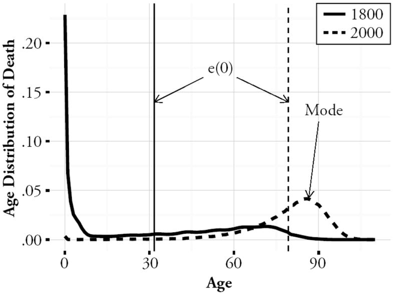
The period age-distributions of death for years 1800 and 2000 in Sweden. The vertical lines show life expectancy at birth, e(0). The modal age at death in adulthood became prominent only after the major process of mortality decline

Since about 1950 in the developed countries, life expectancy has increased consistently, but change in lifespan inequality among countries has varied greatly (Edwards and Tuljapurkar 2005; Engelman et al. 2010; Peltzman 2009; Smits and Monden 2009). This is in striking contrast to the strong negative correlation between changes in life expectancy and lifespan inequality present during the first century of mortality decline (Vaupel et al. 2011). The recent variability of this relationship, we show, results from the very different responses of life expectancy and lifespan inequality to age-specific mortality change. First, we show that in Sweden, the threshold for the variance of age at death increased from childhood in the late eighteenth century to approximately 65 years in 1950 (solid line in Fig. 3). This movement of the threshold altered the relationship between changes in life expectancy and lifespan inequality. Second, we examine the pattern of post–WWII lifespan inequality across many countries, and then focus on Japan, Canada, and the United States. The application of our decomposition to these postwar trajectories of lifespan inequality shows that fluctuations in lifespan inequality resulted primarily from mortality change at young working ages.

Fig. 3.

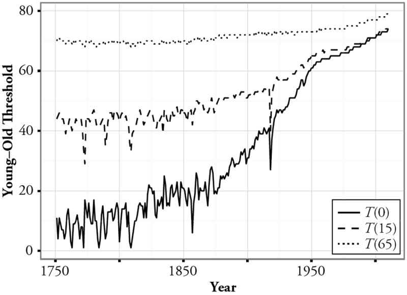
The young–old thresholds, T(A) for A = 0, 15, and 65 years from 1751 to 2011 in Sweden. Note that even in 2011, T(65) was only 14 years above age 65, a considerably smaller gap than for T(0) and T(15)

Results

The Analysis of Change

The variance of age at death after a specified index age A is

$$V(A)=\frac{\mathrm{l}}{l(A)}{\int }_A^{\infty }\mathrm{\phi }(x){[x-M(A)]}^2\mathit{dx},$$ (1)

where M(A) is the mean age at death after age A and is equal to the life expectancy after age A plus A: that is, M(A) = e(A) + A. If we set A = 0, then M(A) = e(0), which is the life expectancy at birth; and the variance, V(0), quantifies the dispersion among deaths at all ages. However, for developed countries, focusing on adult ages can be more informative: for example, using V(15).¹

What is the change in V(A) that results from a proportional mortality reduction at an age x greater than A? Starting from Eq. (1), we find

$$\frac{dV(A)}{d\ln \mathrm{\mu }(x)}=\frac{-2\mathrm{\mu }(x)}{l(A)}{\int }_x^{\infty }l(z)[z-M(A)]\mathit{dz}.$$ (2)

(For details, see Online Resource 1.) The integral in Eq. (2) has a negative term (the contribution from ages between x and M(A)) and a positive term (the contribution from ages above M(A)). If mortality decreases at an age above M(A), the variance V(A) will increase. Now suppose that we reduce mortality at an age below M(A). It is clear from Eq. (2) that reducing mortality at younger ages will gradually cause the negative contribution to dominate, thus decreasing V(A). We therefore define a young–old threshold age, which we call T(A), before which mortality decline decreases V(A) and after which mortality decline increases V(A). The threshold age, T(A), is always less than M(A) because the accumulated increases in V(A) incurred above M(A) must be fully offset by decreases below M(A) before reduction in V(A) can occur.

Hereafter, we refer to the rate of change in Eq. (2) as the sensitivity of V(A). Panel a of Fig. 2 shows the sensitivity of the variance for A = 15, for Sweden in 1950 and 2011. Three features of the plot are typical of mortality in developed countries: (1) mortality decline at ages from 15 to about 65 years decreases V; (2) mortality decline after about 65 years increases V; and (3) there is a threshold age, T(15), at approximately 65 years, that separates “young” ages (at which mortality decline decreases V) from “old” ages (at which mortality decline increases V). The sensitivity of life expectancy e(15) to a proportional mortality decline at age x (Goldman and Lord 1986; Vaupel 1986; Vaupel and Canudas-Romo 2003) is shown for comparison in Fig. 2, panel b. The obvious distinctions are that mortality decline at any age increases life expectancy and that mortality decline close to the threshold has least effect on V. The great difference in the shape of these sensitivities of life expectancy and lifespan inequality—especially below the threshold age—is the critical factor driving their divergent responses to the same age structure of mortality change.

Fig. 2.

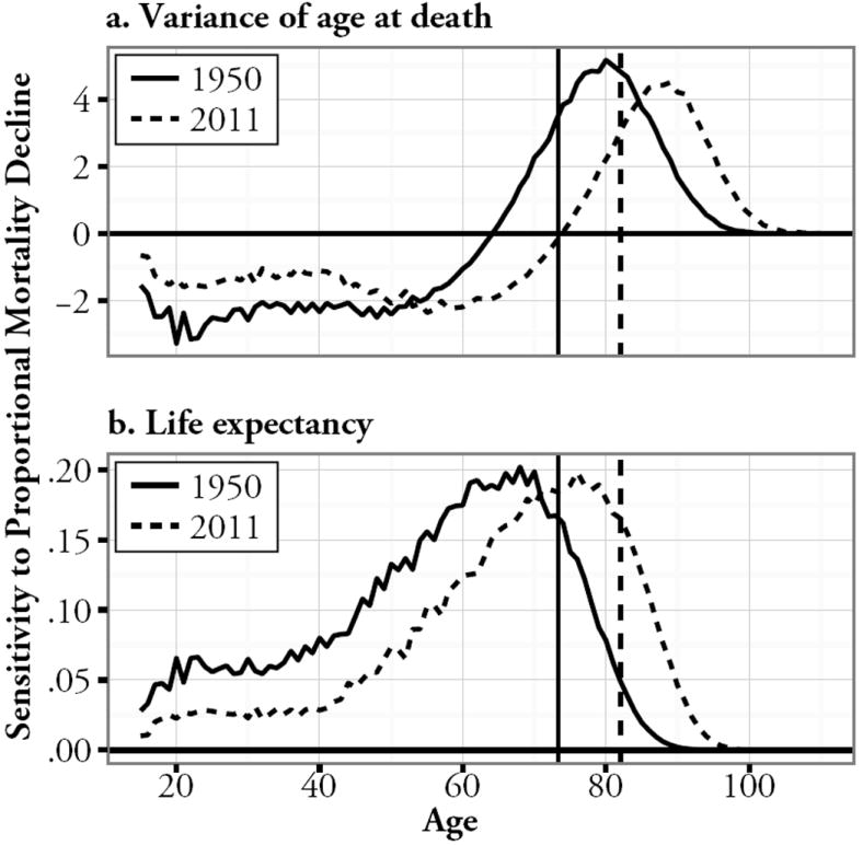
The age-specific sensitivities to proportional mortality reduction in Sweden for 1950 (solid lines) and 2011 (dashed lines) of (a) the variance of age at death after 15 years and (b) the mean age at death (i.e. life expectancy, after this age). The vertical lines show the mean age at death after 15 years, M(15), which equals the life expectancy at age 15 years plus 15 years, e(15) + 15

Long-Term Mortality Change

Sweden was the first country to record ages at death systematically, with records from 1751 to 2011 (Human Mortality Database 2012). These data provide the best opportunity to understand the long-term association of the young–old threshold with changes in lifespan inequality. Figure 3 displays the annual change in the thresholds T(A), for index ages A = 0, 15, and 65 years. Figure 4 shows the concurrent changes in e(A) and V(A).

Fig. 4.

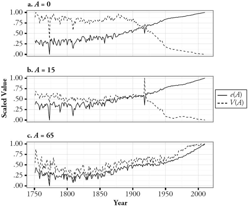
The trajectories of the variance V(A) for A = 0, 15, and 65 years, in panels a, b, and c, respectively, alongside the corresponding trajectories of life expectancy, e(A). Each trajectory has been scaled so that it ranges between 0 and 1 during the study period

To provide some basic intuition on how the threshold depends on the age structure of mortality, we note that a lower bound on the threshold for A = 0 (derived from Eq. (2) in the Online Resource 1) is

$$T(0)\ge 2e(0)-\mathrm{\omega },$$ (3)

where ω is the longest lifespan. In the early years of transition to low mortality, before the late nineteenth century, the lower bound defined by Eq. (3) was below or close to zero. In the first half of the twentieth century, life expectancy increased rapidly, which substantially increased the threshold age: for example, with e(0) = 65 and ω = 100, we have a lower bound at 30 years. More recently, life expectancy has begun to converge on ω. This convergence is commonly known as “rectangularization” of the age structure (Wilmoth and Horiuchi 1999), and it causes the lower bound on the threshold to advance. We now turn to exact values of the young–old threshold.

Before about 1875 in Sweden, he threshold T(0) followed a fluctuating increase to about 20 years (Fig. 3), so only mortality decline in children and very young adults could decrease V. However, V(0) changed little (Fig. 4, panel a), indicating an even distribution of mortality decline below and above the threshold age. From 1875 to about 1950, the threshold advanced to nearly 60 years, so mortality decline at a greater range of young ages could then decrease V. This reinforced the strong negative correlation between changes to life expectancy and lifespan inequality. In this period, V decreased rapidly, and life expectancy increase accelerated, indicating much faster mortality declines below the threshold age. After 1950, the threshold continued advancing to 70–75 years. In this recent period, decreases in V slowed despite continued increases in life expectancy, indicating the switch to more even mortality decline below and above the threshold age.

Increasing the index age after which we measure lifespan inequality advances the young–old threshold. To investigate changes in lifespan inequality among adults, we use an index of 15 years. V(15) did not begin to decrease rapidly until ca. 1925 (Fig. 4, panel b), when the threshold T(15) was 57 years (Fig. 3). That this decrease began about 50 years later than the decrease in V(0) indicates the much later spread of rapid mortality decline from below 15 years to 15–57 years. By 1950, mortality reduction below 15 years had converged the thresholds T(0) and T(15) to 60–65 years. This initiated a period when the distribution of mortality change between working and retired ages was critical in shaping the trajectory of lifespan inequality.

Consider now an index age of 65 years: the obvious feature of mortality change is the consistent positive relationship of changes in life expectancy and lifespan inequality (Fig. 4, panel c). The threshold T(65) was always near 70 years, so only mortality decline at a few young ages could decrease V(65). Therefore, even with mortality reduction by an equal proportion at each age, there was a strong bias for variance increase. The only deviation occurred after 1980, when the trajectory of V(65) flattened while e(65) increased; the threshold was 75 years in 1980. Comparison of mortality change at ages 65–75 years and >75 years showed an abrupt increase in mortality decline among males, which was greatest at 65–75 years (Fig. S1 in Online Resource 1). This decline, which was large enough to overwhelm the bias for variance increase, disrupted the positive correlation between increases in life expectancy and lifespan inequality for the first time since 1751.

The Young–Old Threshold for Mortality in Developed Countries

Now we focus on mortality in developed countries after WWII, when deaths became concentrated at older adult ages. This gave the age distribution of death its characteristic modern pattern, with a well-defined modal age in adulthood (Fig. 1). Before investigating the age-specific drivers of lifespan inequality, we present an approximation to the threshold age that is specific to modern mortality. The modern mortality age pattern is a reasonable fit to the Gompertz model, in which mortality increases with age as

$$\mathrm{\mu }(x)=B{e}^{\mathit{kx}},$$ (4)

where B is the initial level of mortality, and k is the exponential rate of mortality increase. From Eq. (4) (see Online Resource 1 and Tuljapurkar and Edwards (2011)), the mode (m) and standard deviation (σ) of age at death are

$$m\approx \frac{1}{k}\ln \frac{k}{B},$$ (5)

and

$$\mathrm{\sigma }\approx \frac{1}{k}.$$ (6)

Life expectancy is given to a good approximation by

$$e(0)\approx m-\frac{\mathrm{\sigma }}{2},$$ (7)

and our threshold is approximated by

$$T(0)\approx m-\frac{3\mathrm{\sigma }}{2}.$$ (8)

This places the threshold at 1.5 standard deviations of the age at death below the modal age and (using Eq. (7)) 1 standard deviation below life expectancy. The threshold’s advance is therefore driven by increases in both adult life expectancy and modal age at death.

Age-Specific Drivers of Lifespan Inequality Change in Developed Countries

We now focus on the post–WWII changes to V(15) in developed countries, for which the young–old threshold was near ages 60–70. Our analysis shows that changes in lifespan inequality were shaped by striking differences in mortality change for young versus old adults. We begin with a brief international overview: Fig. 5 (solid lines) shows the average trajectories of V(15) for each sex across 40 regional data series from the Human Mortality Database (Vaupel et al. 2011). V(15) fluctuated more for males, and the annual directions of V(15) change were also less regionally consistent in males (Fig. S2, Online Resource 1). Our decomposition (dashed lines) showed that the variance effects of mortality change at young ages (below the threshold) fluctuated more than at old ages (above the threshold), particularly in males. Thus, fluctuations in V(15) clearly come from mortality change at young ages.

Fig. 5.

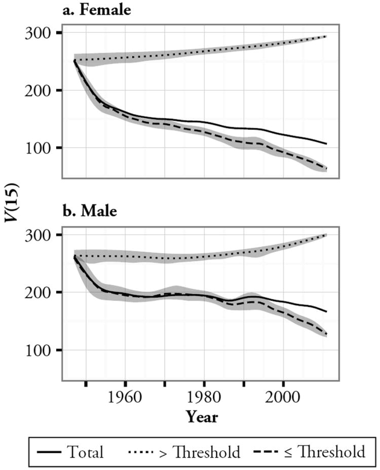
For females (panel a) and males (panel b), solid lines show the average trajectory of the variance of age at death after 15 years, V(15), across 40 regions in the Human Mortality Database (see Table S1 in Online Resource 1 for details). The upper dotted lines show this average trajectory as it would have been only with mortality change above the threshold age, T(15). The lower dashed lines show this for mortality change below the threshold. Note that the lines do not show the variance change at each time t (1947 ≤ t ≤ 2011) but instead show the cumulative effects of mortality change from 1947 to time t. Thus, if W is the annual change in V resulting from mortality change below or above the threshold in each year, the dotted and dashed lines are given by $V(15,1947)+\underset{1947}{\overset{t}{\int }}W(15,u)\mathit{du}$. The gray shading around the dotted and dashed lines shows the annual 95 % range of variability among regions in each component of change

We now examine in more detail Japan, Canada, and the United States, which illustrate the main features of post-1947 mortality change in developed countries: relatively steady increase in life expectancy (Fig. S3, Online Resource 1) but large fluctuation in V (Fig. S4, Online Resource 1). We focus on the slowing of variance decrease and, in some regions, onset of variance increase in the 1980s. The United States in particular showed a striking variance increase in the early 1980s. The threshold ages were close to the conventional age of retirement, although there was a steady increase in thresholds over time—by a maximum of 28 years in Japanese females (Fig. S5, Online Resource 1).

Japan

Figure 6 shows how mortality change at young ages (below the threshold) and at old ages (above the threshold) generated the contrasting variance trajectories of each country.² In Japan, each sex followed the same basic trajectory of variance change: a rapid decrease from 1947 to about 1975, and an increase after about 1990 (Fig. 6, panels a and b). The sexes differed in that V initially decreased faster for females, and the reversal from variance decrease to increase was earlier for females. Our decomposition shows that the initial variance decrease before 1977 was driven by the variance contracting effects of mortality decline at young ages, which dominated the effects of mortality decline at old ages (Fig. 6, panels a and b). Around the 1980s, these opposing effects reached a rough equilibrium, and thus V changed little. However, after about 1990, the negative effects of mortality decline at young ages weakened further, leading the positive effects of mortality decline at old ages to dominate. This shift in the focus of mortality decline to old ages consequently led V to increase (Fig. S7, Online Resource 1).

Fig. 6.

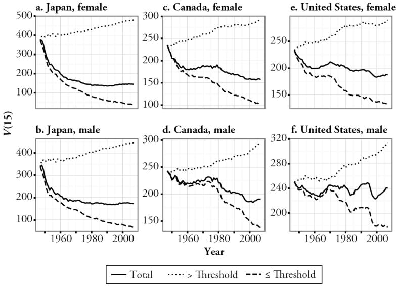
Decomposition of the variance of age at death after 15 years, V(15) into the effects of mortality change below and above the young–old threshold age, T(15). Solid lines show the overall variance change, dashed lines show the change produced from ages below the threshold, and dotted lines indicate the change produced from ages above the threshold. We show separate decompositions for females and males in Japan (panels a and b), Canada (panels c and d), and the United States (panels e and f) from 1947 to 2007. Lines show the cumulative variance effects of mortality change plus V(15, 1947) (see details in the legend of Fig. 5)

Canada and the United States

In Canada and the United States, the variance changes after 1947 were much smaller than in Japan (note the difference in y-axis scales in Fig. 6). Prior to 1983, Canada and the United States followed similar trajectories, each with little net variance change. However, after 1983, V increased and continued to fluctuate in the United States but began a rapid and consistent decrease in Canada. The result was that from 1983 to 2007, the Canadian variance (for females and males, respectively) changed from 8 % and 9 % lower than that for the United States to 20 % and 15 % lower.

We now focus on the period 1983–1994, which captures the major variance divergence between Canada and the United States (Fig. 6, panels c–f). In Canada, mortality decline at young ages produced percentage variance changes of −10.8 % for females and −10.1 % for males (Fig. 6, panels c and d). From old ages, the changes were 1.0 % in females and 2.9 % in males. In the United States, mortality change at young ages produced variance changes of −3.3 % in females and 3.6 % in males; and from old ages, 1.5 % and 4.8 %, respectively (Fig. 6, panels e and f). Thus, owing mainly to differences in male mortality change, the United States produced a larger component of variance increase from old ages but a much smaller component of variance decrease (and for males, variance increase) from young ages.

How did mortality change differ at young ages between Canada and the United States? In the latter, male mortality increased at ages 15–22 and 27–45, with increases greater than 30 % at 34–37 years (Fig. 7). U.S. females showed a pattern that was similar but of smaller magnitude (a maximum increase of 20 % at 35 years). By contrast, mortality increase for Canadian males was limited to ages 32–40, with a maximum increase of 17 %; mortality generally declined for Canadian females. The age-specific changes in mortality, therefore, differed most between Canada and the United States at young working ages, particularly among males. As a result, variance diverged sharply between Canada and the United States. When looked at in terms of life expectancy, this divergence is almost completely missed (Fig. S3, Online Resource 1). Thus, diagnosing mortality trends based on life expectancy alone is inadequate, and lifespan inequality should feature routinely in demographic monitoring.

Fig. 7.

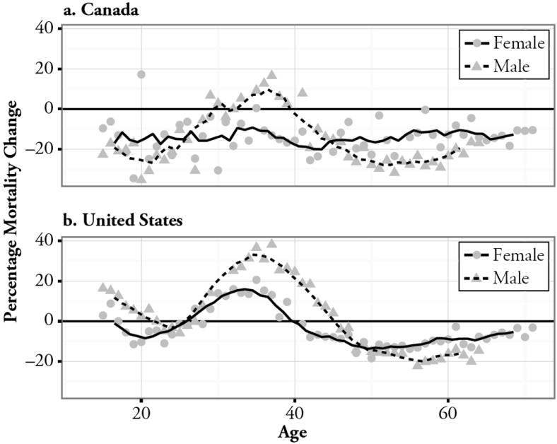
The percentage changes to the central one-year death rates at ages from 15 years to the average young–old threshold for females (71 years) and males (64 years) between 1983 and 1994 in Canada (panel 1) and the United States (panel b). Separate lines show the five-year moving averages of the percentage change for females and males

Discussion

This article shows how change in lifespan inequality, as measured by V, depends strongly on the balance of mortality change around a young–old threshold. The threshold advances with increases in life expectancy, the modal age at death, and with the compression of mortality into a narrower range of ages. Before about 1950, changes to life expectancy and lifespan inequality had a strong negative correlation (Smits and Monden 2009; Vaupel et al. 2011), which arose because the emphasis of mortality decline was on ages below the threshold (Vaupel et al. 2011). Since 1950, lifespan inequality decrease has slowed and occasionally even reversed. We show that the post–WWII fluctuations in lifespan inequality were driven by fluctuations in mortality at young working ages, below the threshold age, whereas mortality decline was relatively consistent at old ages. The implication of these trends is clear: if mortality at young ages continues to fluctuate and mortality at old ages continues its steady decline, lifespan inequality increases will become more common.

But what drives these trajectories of age-specific mortality, causing them to vary both within and among countries? This question brings the focus of our attention to the social determinants of mortality (Graham 2009), and so to the realization that international divergence in lifespan inequality must largely be due to divergence in age patterns of the social determinants. Mortality is ultimately associated with education, income, social support (from family or public institutions, including the provision of healthcare), lifestyle, disease, and living conditions. These interact with the proximate, health-related causes of death at each age to generate lifespan inequality (Edwards and Tuljapurkar 2005; Nau and Firebaugh 2012; Shkolnikov et al. 2011). For example, Japanese development after 1947, including the start of universal healthcare in 1961, generated rapid mortality decline at mainly working ages. It is possible that this rapid progress against mortality gradually left the remaining causes of death in young adults in the category of those causes that are difficult to prevent. However, society—and hence the array of social determinants—was also changing, characterized by widening differences in mortality by education and income, particularly among working-aged males (Fukuda et al. 2004; Kagamimori et al. 2009). These social changes could also have contributed to the slowing of mortality declines in young adults: for example, if progress against the social determinants became limited to the most-educated or most-affluent.

A great deal of research is aimed at understanding why young adult mortality remains high in the United States compared with other high-income countries (Crimmins et al. 2011; IOM 2012). One source may be high geographic disparity in young adult mortality within the United States. For example, Cullen et al. (2012) showed that mortality differences below age 70 among U.S. counties and racial groups resulted largely from differences in education and income, particularly for males (see also Backlund et al. 2007; Crimmins et al. 2009). Current evidence also suggests that life expectancy differences between educational groups in the United States have widened in recent decades (Olshansky et al. 2012). A part of this variation is likely due to differences in healthcare access among young adults (Crimmins et al. 2011). Indeed, any explanation of trends in U.S. mortality must address the hypothesis that the correlation of social deprivation with low healthcare access raises the sensitivity of working-age mortality to macroeconomic change. In the United States, healthcare access at working ages depends largely on employer-provided health insurance; in 1994, 18.6 % of non-elderly adults in the United States had no health insurance (Holahan and Kim 2000). Being without health insurance limits care, particularly preventive care at young ages (Lasser et al. 2006), with evidence for consequently higher mortality (Wilper et al. 2009). The 1980s lifespan inequality divergence between Canada and the United States could be explained by such social factors: it is not possible to exclude the explanation that macroeconomic change resulted in more people in the United States in poor health and with no social safety net to ensure appropriate healthcare (Brenner and Mooney 1983; Siddiqi and Hertzman 2007). A slightly different understanding is gained by looking at the common causes of death at young, working ages (Harper et al. 2007; Nau and Firebaugh 2012). Harper et al. (2007) showed that in the United States in the 1980s, mortality among young adults rose, and the black-white gap in life expectancy increased because of differential increases in mortality from human immunodeficiency virus (HIV), heart disease, and homicide. HIV became prevalent in the 1980s and early 1990s, particularly among males aged 25–64, more so in the United States than in Canada (Armstrong et al. 1999; UNAIDS 2013). Nau and Firebaugh (2012) also highlighted heart disease and homicides as key contributors to the high variance of age at death in the United States. Heart disease is a leading cause of premature death; accidents and homicides, although being less common causes, also account for a high proportion of deaths at the youngest adult ages, where (as we show) the variance is highly sensitive to mortality change.

Alternate Inequality Metrics

Several established metrics of lifespan inequality exist (van Raalte and Caswell 2013). For the same mortality data, the young–old threshold can differ widely among these metrics; for example, by around 20 years, between V and the metric known as “lifespan disparity,” or e^† (Zhang and Vaupel 2009). Our results indicate that the major post–WWII mortality changes occurred outside the zone of threshold disagreement among metrics, indicating that our qualitative conclusions are robust to the choice of metric. We use V for three reasons: it is easily understood and interpreted as a measure of relative dispersion, is easily decomposed (Edwards 2011; Edwards and Tuljapurkar 2005; Nau and Firebaugh 2012), and finds direct use in analyzing the demographic and economic consequences of mortality change (Edwards 2012; Schindler et al. 2012; Tuljapurkar 2008).

The Future

Because the young–old threshold in developed countries is now approaching 75–80 years (Fig. 2a), only mortality decline at the oldest retired ages can increase lifespan inequality. Given the ongoing fluctuation of social gradients in age-specific health and mortality, as well as the importance of social gradients for generating lifespan inequality (Cullen et al. 2012; Olshansky et al. 2012), we suggest that future work focus on the population-level effects of mortality change within specific social groups (Edwards 2011; Nau and Firebaugh 2012; Shkolnikov et al. 2011; van Raalte et al. 2011, 2012). The great good of development has been the consistent improvement of medical technology and care for the elderly, reflected in steadily declining old-age mortality (Vaupel 2010). However, our results suggest that without comparable progress in combating young-adult mortality, through action on the social determinants, mortality change is unlikely to follow the historical pattern of rising life expectancy and falling lifespan inequality. Hence, we should be prepared for increases in lifespan inequality to become a more common feature of demographic change.

Appendix: Materials and Methods

We downloaded our data from the Human Mortality Database (HMD) in January 2013 (Human Mortality Database 2012).³ For international comparisons, we used the same data series as Vaupel et al. (2011). Table S1 (Online Resource 1) shows the range of years between 1947 and 2011 that is covered by these data. We conducted all calculations in the R environment (R Development Core Team (2012)). Online Resource 1 gives the derivation of each formula presented. For our age decomposition of change in V(15), we adapted Eq. (2) to

$$\frac{\mathit{dV}(15)}{\mathit{dt}}=-2{\int }_{15}^{\infty }\frac{a(x)\mathrm{\mu }(x)}{l(15)}{\int }_x^{\infty }l(z)[z-M(15)]\mathit{dz\; dx},$$ (9)

which gives the change in V(15) over time interval dt. The observed proportional changes in age-specific mortality, a(x), between years t and t + 1 were computed as

$$a(x)=\frac{\mathrm{\mu }(x,t+1)-\mathrm{\mu }(x,t)}{\mathrm{\mu }(x,t)}.$$ (10)

To convert time in these formulae to discrete one-year intervals, we discretized the probability density function of age at death, considered survivorship to the midpoint of each age interval, and substituted instantaneous mortality for central death rates. We counted age in one-year intervals starting from 0.5 years. Where we present mortality change over wider age intervals, we computed a weighted average of the one-year central death rates in each interval, using the probability of survival to each age as weights (Ahmad et al. 2001).

References

- Ahmad O, Boschi-Pinto C, Lopez AD, Murray CJL, Lozano R, Inoue M. Age standardization of rates: A new WHO standard. Geneva, Switzerland: World Health Organization; 2001. [Google Scholar]
- Armstrong GL, Conn LA, Pinner RW. Trends in infectious disease mortality in the United States during the 20th century. Journal of the American Medical Association. 1999;281:61–66. doi: 10.1001/jama.281.1.61. [DOI] [PubMed] [Google Scholar]
- Backlund E, Rowe G, Lynch J, Wolfson MC, Kaplan GA, Sorlie PD. Income inequality and mortality: A multilevel prospective study of 521248 individuals in 50 US states. International Journal of Epidemiology. 2007;36:590–596. doi: 10.1093/ije/dym012. [DOI] [PubMed] [Google Scholar]
- Bongaarts J. Long-range trends in adult mortality: Models and projection methods. Demography. 2005;42:23–49. doi: 10.1353/dem.2005.0003. [DOI] [PubMed] [Google Scholar]
- Brenner MH, Mooney A. Unemployment and health in the context of economic change. Social Science & Medicine. 1983;17:1125–1138. doi: 10.1016/0277-9536(83)90005-9. [DOI] [PubMed] [Google Scholar]
- Canudas-Romo V. The modal age at death and the shifting mortality hypothesis. Demographic Research. 2008;19(article 30):1179–1204. doi: 10.4054/DemRes.2008.19.30. [DOI] [Google Scholar]
- Caswell H. Stage, age and individual stochasticity in demography. Oikos. 2009;118:1763–1782. [Google Scholar]
- Cheung SLK, Robine JM, Tu EJC, Caselli G. Three dimensions of the survival curve: Horizontalization, verticalization, and longevity extension. Demography. 2005;42:243–258. doi: 10.1353/dem.2005.0012. [DOI] [PubMed] [Google Scholar]
- Crimmins EM, Kim JK, Seeman TE. Poverty and biological risk: The earlier “aging” of the poor. Journals of Gerontology Series A–Biological Sciences and Medical Sciences. 2009;64:286–292. doi: 10.1093/gerona/gln010. [DOI] [PMC free article] [PubMed] [Google Scholar]
- Crimmins EM, Preston SH, Cohen B. Explaining divergent levels of longevity in high-income countries. Washington, DC: National Academies Press; 2011. [PubMed] [Google Scholar]
- Cullen MR, Cummins C, Fuchs VR. Geographic and racial variation in premature mortality in the U.S.: Analyzing the disparities. Plos One. 2012;7(4):e32930. doi: 10.1371/journal.pone.0032930. [DOI] [PMC free article] [PubMed] [Google Scholar]
- Cutler D, Deaton A, Lleras-Muney A. The determinants of mortality. Journal of Economic Perspectives. 2006;20:97–120. [Google Scholar]
- Edwards RD. Changes in world inequality in length of life: 1970–2000. Population and Development Review. 2011;37:499–528. doi: 10.1111/j.1728-4457.2011.00432.x. [DOI] [PubMed] [Google Scholar]
- Edwards RD. The cost of uncertain life span. Journal of Population Economics. 2012;25:1–38. doi: 10.1007/s00148-012-0405-0. [DOI] [PMC free article] [PubMed] [Google Scholar]
- Edwards RD, Tuljapurkar S. Inequality in life spans and a new perspective on mortality convergence across industrialized countries. Population and Development Review. 2005;31:645–674. [Google Scholar]
- Engelman M, Canudas-Romo V, Agree EM. The implications of increased survivorship for mortality variation in aging populations. Population and Development Review. 2010;36:511–539. doi: 10.1111/j.1728-4457.2010.00344.x. [DOI] [PubMed] [Google Scholar]
- Fukuda Y, Nakamura K, Takano T. Municipal socioeconomic status and mortality in Japan: Sex and age differences, and trends in 1973–1998. Social Science & Medicine. 2004;59:2435–2445. doi: 10.1016/j.socscimed.2004.04.012. [DOI] [PubMed] [Google Scholar]
- Goldman N, Lord G. A new look at entropy and the life table. Demography. 1986;23:275–282. [PubMed] [Google Scholar]
- Graham H. Health inequalities, social determinants and public health policy. Policy and Politics. 2009;37:463–479. [Google Scholar]
- Harper S, Lynch J, Burris S, Davey Smith G. Trends in the black-white life expectancy gap in the United States, 1983–2003. Journal of the American Medican Association. 2007;297:1224–1232. doi: 10.1001/jama.297.11.1224. [DOI] [PubMed] [Google Scholar]
- Holahan J, Kim J. Why does the number of uninsured Americans continue to grow? Health Affairs. 2000;19:188–196. doi: 10.1377/hlthaff.19.4.188. [DOI] [PubMed] [Google Scholar]
- Horiuchi S, Wilmoth JR, Pletcher SD. A decomposition method based on a model of continuous change. Demography. 2008;45:785–801. doi: 10.1353/dem.0.0033. [DOI] [PMC free article] [PubMed] [Google Scholar]
- Human Mortality Database. University of California, Berkeley, and Max Planck Institute for Demographic Research (Germany) 2012 Retrieved from www.mortality.org or www.humanmortality.de.
- IOM. How far have we come in reducing health disparities?: Progress since 2000 (Institute of Medicine workshop summary) Washington, DC: The National Academies Press; 2012. [PubMed] [Google Scholar]
- Kagamimori S, Gaina A, Nasermoaddeli A. Socioeconomic status and health in the Japanese population. Social Science & Medicine. 2009;68:2152–2160. doi: 10.1016/j.socscimed.2009.03.030. [DOI] [PubMed] [Google Scholar]
- Keyfitz N. Applied mathematical demography. New York, NY: Wiley-Interscience; 1977. [Google Scholar]
- Lasser KE, Himmelstein DU, Woolhandler S. Access to care, health status, and health disparities in the United States and Canada: Results of a cross-national population-based survey. American Journal of Public Health. 2006;96:1300–1307. doi: 10.2105/AJPH.2004.059402. [DOI] [PMC free article] [PubMed] [Google Scholar]
- Lee RD, Carter LR. Modeling and forecasting United-States mortality. Journal of the American Statistical Association. 1992;87:659–671. [Google Scholar]
- Nau C, Firebaugh G. A new method for determining why length of life is more unequal in some populations than in others. Demography. 2012;49:1207–1230. doi: 10.1007/s13524-012-0133-9. [DOI] [PMC free article] [PubMed] [Google Scholar]
- Olshansky SJ, Antonucci T, Berkman L, Binstock RH, Boersch-Supan A, Cacioppo JT, Rowe J, et al. Differences in life expectancy due to race and educational differences are widening, and many may not catch up. Health Affairs (Project HOPE) 2012;31:1803–1813. doi: 10.1377/hlthaff.2011.0746. [DOI] [PubMed] [Google Scholar]
- Peltzman S. Mortality inequality. Journal of Economic Perspectives. 2009;23:175–190. doi: 10.1257/jep.23.4.175. [DOI] [PubMed] [Google Scholar]
- R Development Core Team. R: A language and environment for statistical computing. Vienna, Austria: R Foundation for Statistical Computing; 2012. [Google Scholar]
- Schindler S, Tuljapurkar S, Gaillard J-M, Coulson T. Linking the population growth rate and the age-at-death distribution. Theoretical Population Biology. 2012;82:244–252. doi: 10.1016/j.tpb.2012.09.003. [DOI] [PMC free article] [PubMed] [Google Scholar]
- Shkolnikov VM, Andreev EM, Zhang Z, Oeppen J, Vaupel JW. Losses of expected lifetime in the United States and other developed countries: Methods and empirical analyses. Demography. 2011;48:211–239. doi: 10.1007/s13524-011-0015-6. [DOI] [PubMed] [Google Scholar]
- Siddiqi A, Hertzman C. Towards an epidemiological understanding of the effects of long-term institutional changes on population health: A case study of Canada versus the USA. Social Science & Medicine. 2007;64:589–603. doi: 10.1016/j.socscimed.2006.09.034. [DOI] [PubMed] [Google Scholar]
- Smits J, Monden C. Length of life inequality around the globe. Social Science & Medicine. 2009;68:1114–1123. doi: 10.1016/j.socscimed.2008.12.034. [DOI] [PubMed] [Google Scholar]
- Tuljapurkar S. Mortality declines, longevity risk and aging. Asia-Pacific Journal of Risk and Insurance. 2008;3(1):37–51. [Google Scholar]
- Tuljapurkar S, Edwards RD. Variance in death and its implications for modeling and forecasting mortality. Demographic Research. 2011;24(article 21):497–526. doi: 10.4054/DemRes.2001.24.21. [DOI] [PMC free article] [PubMed] [Google Scholar]
- Tuljapurkar S, Li N, Boe C. A universal pattern of mortality decline in the G7 countries. Nature. 2000;405:789–792. doi: 10.1038/35015561. [DOI] [PubMed] [Google Scholar]
- UNAIDS. AIDSinfo: Epidemiological status [Data file] 2013 Retrieved from http://www.unaids.org/en/dataanalysis/datatools/aidsinfo/
- van Raalte AA, Caswell H. Perturbation analysis of indices of lifespan variability. Demography. 2013;50:1615–1640. doi: 10.1007/s13524-013-0223-3. [DOI] [PubMed] [Google Scholar]
- van Raalte AA, Kunst AE, Deboosere P, Leinsalu M, Lundberg O, Martikainen P, Mackenbach JP, et al. More variation in lifespan in lower educated groups: Evidence from 10 European countries. International Journal of Epidemiology. 2011;40:1703–1714. doi: 10.1093/ije/dyr146. [DOI] [PubMed] [Google Scholar]
- van Raalte AA, Kunst AE, Lundberg O, Leinsalu M, Martikainen P, Artnik B, Mackenbach JP, et al. The contribution of educational inequalities to lifespan variation. Population Health Metrics. 2012;10 doi: 10.1186/1478-7954-10-3. [DOI] [PMC free article] [PubMed] [Google Scholar]
- Vaupel JW. How change in age-specific mortality affects life expectancy. Population Studies. 1986;40:147–157. doi: 10.1080/0032472031000141896. [DOI] [PubMed] [Google Scholar]
- Vaupel JW. Biodemography of human ageing. Nature. 2010;464:536–542. doi: 10.1038/nature08984. [DOI] [PMC free article] [PubMed] [Google Scholar]
- Vaupel JW, Canudas-Romo V. Decomposing change in life expectancy: A bouquet of formulas in honor of Nathan Keyfitz’s 90th birthday. Demography. 2003;40:201–216. doi: 10.1353/dem.2003.0018. [DOI] [PubMed] [Google Scholar]
- Vaupel JW, Zhang Z, van Raalte AA. Life expectancy and disparity: An international comparison of life table data. BMJ Open. 2011;1(1):e000128. doi: 10.1136/bmjopen-2011-000128. [DOI] [PMC free article] [PubMed] [Google Scholar]
- Wilmoth JR, Horiuchi S. Rectangularization revisited: Variability of age at death within human populations. Demography. 1999;36:475–495. [PubMed] [Google Scholar]
- Wilper AP, Woolhandler S, Lasser KE, McCormick D, Bor DH, Himmelstein DU. Health insurance and mortality in US adults. American Journal of Public Health. 2009;99:2289–2295. doi: 10.2105/AJPH.2008.157685. [DOI] [PMC free article] [PubMed] [Google Scholar]
- Zhang Z, Vaupel JW. The age separating early deaths from late deaths. Demographic Research. 2009;20(article 29):721–730. doi:10.4054.DemRes.2009.20.29. [Google Scholar]
Associated Data
This section collects any data citations, data availability statements, or supplementary materials included in this article.