A wavelet method for modeling and despiking motion artifacts from resting-state fMRI time series

Abstract

The impact of in-scanner head movement on functional magnetic resonance imaging (fMRI) signals has long been established as undesirable. These effects have been traditionally corrected by methods such as linear regression of head movement parameters. However, a number of recent independent studies have demonstrated that these techniques are insufficient to remove motion confounds, and that even small movements can spuriously bias estimates of functional connectivity. Here we propose a new data-driven, spatially-adaptive, wavelet-based method for identifying, modeling, and removing non-stationary events in fMRI time series, caused by head movement, without the need for data scrubbing. This method involves the addition of just one extra step, the Wavelet Despike, in standard pre-processing pipelines. With this method, we demonstrate robust removal of a range of different motion artifacts and motion-related biases including distance-dependent connectivity artifacts, at a group and single-subject level, using a range of previously published and new diagnostic measures. The Wavelet Despike is able to accommodate the substantial spatial and temporal heterogeneity of motion artifacts and can consequently remove a range of high and low frequency artifacts from fMRI time series, that may be linearly or non-linearly related to physical movements. Our methods are demonstrated by the analysis of three cohorts of resting-state fMRI data, including two high-motion datasets: a previously published dataset on children (N = 22) and a new dataset on adults with stimulant drug dependence (N = 40). We conclude that there is a real risk of motion-related bias in connectivity analysis of fMRI data, but that this risk is generally manageable, by effective time series denoising strategies designed to attenuate synchronized signal transients induced by abrupt head movements. The Wavelet Despiking software described in this article is freely available for download at www.brainwavelet.org.

Graphical abstract

Highlights

• •Motion artifacts in fMRI data may manifest in complex temporal and spatial patterns.
• •These artifacts are hard to model, and are often poorly denoised by popular methods.
• •Wavelet-based despiking is a novel, data driven, locally adaptive denoising method.
• •Wavelet Despiking can remove linear, non-linear, high and low frequency artifacts.
• •Wavelet Despiking attenuates motion-induced bias in functional connectivity.

Introduction

Head movement has long been known to induce undesirable, artifactual effects on functional magnetic resonance imaging (fMRI) signals (Biswal et al., 1995; Bullmore et al., 1999a; Friston et al., 1996; Hajnal et al., 1994). Head movement artifacts can originate from a number of sources including physiological noise caused by respiration and cardiac pulsations, slow involuntary drifts in head position, and briefer ‘spike-like’ movements. Notably, it is the latter that are most damaging to fMRI data, as they can induce substantial spin-history and slice-readout artifacts, and cause geometric deformation of the brain (Friston et al., 1996; Hajnal et al., 1994).

Traditional methods for correcting primary motion artifacts, such as misalignment of image position and geometric deformation of the brain, include volume realignment using a rigid-body or affine transform. Correction for secondary motion artifacts, such as field inhomogeneity changes and spin-history effects, is more difficult. Commonly used methods to correct some of these include linear regression of head movement parameters (Bullmore et al., 1999a), or component filtering after Independent Component Analysis (Beckmann and Smith, 2005). These methods are often able to remove some, but not all of these secondary artifacts. Notably, spin-history effects can be difficult to remove. The difficulty in modeling these secondary effects on fMRI time series from the movement parameter information available, may be further complicated by a number of factors, including, but not limited to, subject movement in between frames, which may result in substantial non-linear and non-spatially-uniform effects in time series. As demonstrated concurrently by three recent independent studies (Power et al., 2012; Satterthwaite et al., 2012; Van Dijk et al., 2012), and as demonstrated by a number of subsequent studies (Bright and Murphy, 2013; Mowinckel et al., 2012; Satterthwaite et al., 2013; Tyszka et al., 2013; Yan et al., 2013), even small head movements in the range of 0.5 to 1 mm can induce systematic biases in correlation strength between nearby brain regions. As suggested by these studies, the more subtle effects may be difficult to remove with traditional methods, particularly in groups of patients and children, where spike-like head movements are more frequent, are likely to be larger in amplitude, and often correlate with the feature being studied, such as the age of the subject or severity of the disease.

In light of this problem, a number of methods have been proposed to ameliorate the observed motion-induced biases in the estimation of functional connectivity. These have largely focused around data ‘scrubbing’ (originally proposed by Power et al. (2012)), which involves the removal of motion-affected frames of data from pre-processed time series, guided by head movement and signal change parameters. A number of more recent articles have suggested improvements on the original method, including: (i) removing affected frames prior to Fourier filtering and interpolating the missing data to prevent temporal leakage of artifact (Carp, 2012), (ii) scrubbing within regression (‘spike regression’, Satterthwaite et al., 2013) and (iii), use of higher-order, or Volterra-expanded, confound regressors with or without data scrubbing, such as the 36-parameter model proposed by Satterthwaite et al. (2013), and the 24-parameter autoregressive model proposed by Yan et al. (2013).

Here we propose a new data-driven, wavelet-based method for modeling and removing secondary motion artifacts from fMRI data, without the need for data scrubbing. This unsupervised method detects non-stationary events, caused by movement, as chains of scale-invariant maximal or minimal wavelet coefficients, and despikes these from voxel time series. Importantly, because the algorithm can identify non-stationary events across different frequencies, it is able to remove slower, prolonged, motion artifacts such as spin-history type effects, as well as higher frequency events such as step changes in signal intensity and spikes. We demonstrate, at a single-subject and group level, using a number of previously published and new diagnostic measures, that this method provides benefits over more standard despiking procedures, and is more successful at removing motion artifacts than previously published regression methods, because there is no dependence on a predefined model explaining the relationship between physical movements and effects of fMRI signal. This property also affords the algorithm spatial adaptivity. As a result, it is more effective at removing a wide range of movement-induced artifacts, which can themselves be spatially heterogeneous in nature.

We illustrate these new methods in three cohorts of single-echo fMRI data, including two high-motion cohorts: a previously published group of children (N = 22; Power et al., 2012); and a new dataset on adults with stimulant drug dependence (N = 40). We also analyze a relatively low-motion cohort: a new healthy adult dataset (N = 45). We conclude that the addition of the wavelet-based despiking step prior to confound signal regression during pre-processing, provides a benefit over use of more standard despiking algorithms, and enables better removal of motion artifacts from high-motion cohorts than previously described regression-only and/or scrubbing methods.

Materials and methods

Subjects

Resting-state fMRI data from three cohorts of subjects were studied. Cohort 1 is a previously published cohort of 22 children (Power et al., 2012) average age 8.5. All subjects gave assent with parental consent as approved by the Washington University Human Studies Committee. Cohort 2 is a group of 40 stimulant-dependent adults that met the DSM-IV criteria for stimulant dependence, average age 34.8 years. Cohort 3 is a group of 45 healthy biological siblings of cohort 2 subjects, average age 32.3 years. From the original cohort, 5 subjects were excluded from cohorts 2, and 4 from cohort 3 due to the presence of acquisition errors or brain clipping. These subjects are not included in the total cohort numbers. Data collection for cohorts 2 and 3 was approved by the Cambridge Research Ethics Committee (REC08/H0308/310), and all subjects provided written informed consent prior to enrolment. Table 1 contains further details on these cohorts. Cohort 1 was used to demonstrate results for all analyses, except those presented in Inline Supplementary Figs. S5 and S6, and Table 1, where results from all three cohorts were used.

Table 1.

Summary of cohorts. *These subjects were excluded for excessive amount of head movement (see the Subject exclusion criteria section). In addition, 5 subjects were excluded from cohort 2 and 4 subjects from cohort 3 during pre-processing due to the presence of acquisition errors or brain clipping. These latter subjects are not included in the cohort totals represented by [N]. Superscript numbers represent scrubbing criteria used in: ¹Yan et al. (2013), ²Power et al. (2013), and ³Satterthwaite et al. (2013).

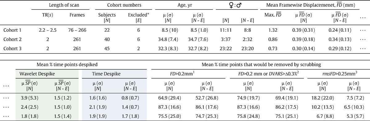
Fig. S5.

Effects of despiking on distance-dependent connectivity bias, as measured by the ‘∆R plot’. This figure shows group-level ∆R plots (see the Distance-dependent movement artifact diagnostics section) across all subjects in the three cohorts analyzed. Column 1 represents the pre-processing scenario where the Time Despike was applied prior to 13-parameter confound regression, and column 2 represents the scenario where the Wavelet Despike was applied prior to 13-parameter confound regression (see Fig. 1). In each case, the ∆R plots were computed after fully pre-processing the time series, including band-pass filtering (0.009 < f < 0.08 Hz) in the last step.

Fig. S6.

Effects of despiking on distance-dependent connectivity bias, as measured by the ‘motion-correlation plot’. This figure shows group-level motion-correlation plots (see the Distance-dependent movement artifact diagnostics section) across all subjects in the three cohorts analyzed. Column 1 represents the pre-processing scenario where the Time Despike was applied prior to 13-parameter confound regression, and column 2 represents the scenario where the Wavelet Despike was applied prior to 13-parameter confound regression (see Fig. 1). In each case, the motion-correlation plots were computed after fully pre-processing the time series, including band-pass filtering at 0.009 < f < 0.08 Hz. Histograms adjacent to the respective motion-correlation plots represent the null distribution of mean correlation between connectivity and motion (the mean y axis value averaged across all distances for the adjacent motion-correlation plot) that could arise by chance. This distribution was calculated by randomly permuting the movement estimate for each subject 1000 times, each time calculating the mean correlation of the resultant random motion-correlation plot. The mean values above each histogram represent the mean correlation with movement across all distances, from the true motion correlation plots (pictured to the left of the histograms). Starred means represent those significantly different from the null distribution at p = 0.05.

Resting-state fMRI data from three cohorts of subjects were studied. Cohort 1 is a previously published cohort of 22 children (Power et al., 2012) average age 8.5. All subjects gave assent with parental consent as approved by the Washington University Human Studies Committee. Cohort 2 is a group of 40 stimulant-dependent adults that met the DSM-IV criteria for stimulant dependence, average age 34.8 years. Cohort 3 is a group of 45 healthy biological siblings of cohort 2 subjects, average age 32.3 years. From the original cohort, 5 subjects were excluded from cohort 2, and 4 from cohort 3 due to the presence of acquisition errors or brain clipping. These subjects are not included in the total cohort numbers. Data collection for cohorts 2 and 3 was approved by the Cambridge Research Ethics Committee (REC08/H0308/310), and all subjects provided written informed consent prior to enrolment. Table 1 contains further details on these cohorts. Cohort 1 was used to demonstrate results for all analyses, except those presented in Inline Supplementary Figs. S5 and S6, and Table 1, where results from all three cohorts were used.

FMRI data acquisition

Cohort 1 data (Power et al., 2012) was obtained from Washington University at St. Louis, and the surrounding areas. Subjects were scanned on a Siemens MAGNETOM Tim Trio 3.0 T Scanner. Each dataset comprised a T1 weighted MPRAGE structural image (TE = 3.06 ms, TR-partition = 2.4 s, TI = 1000 ms, flip angle = 8°) with a voxel resolution of 1.0 × 1.0 × 1.0 mm, and a BOLD functional image, acquired using a whole-brain gradient echo echo-planar (EPI) sequence with interleaved slice acquisition (TR = 2.2–2.5 s, TE = 27 ms, flip angle = 90°), and with voxel dimensions of 4.0 × 4.0 × 4.0 mm. For some subjects, independent runs were concatenated, as in Power et al. (2012). Where this was the case, subject data was concatenated at a regional level, after parcellation (see the Definition of regional time series section below), as on average, concatenated scans were taken 15.5 days apart, and therefore there was often substantial variability in voxel numbers, which made it difficult to concatenate scans reliably during functional image pre-processing.

Cohorts 2 and 3 were scanned at the Wolfson Brain Imaging Centre, Cambridge, UK, using a Siemens MAGNETOM Tim Trio 3.0 T Scanner. For each subject, a T1-weighted sagittal MPRAGE structural image was acquired at the start of the scanning session (TE = 2.98 ms, TR = 2300 ms, TI = 900 ms, flip angle = 9°, FOV = 256 mm), with a voxel resolution of 1.0 × 1.0 × 1.0 mm. BOLD functional images were acquired with eyes closed, using a whole-brain gradient echo echo-planar (EPI) sequence of 261 volumes with interleaved slice acquisition (TR = 2000 ms, TE = 30 ms, flip angle = 78°, FOV = 192 mm, slice thickness/gap = 3 mm/0 mm), and with voxel dimensions of 3.0 × 3.0 × 3.0 mm.

Functional image pre-processing

Functional and structural images were processed using AFNI/SUMA (http://afni.nimh.nih.gov/) and FSL (http://fsl.fmrib.ox.ac.uk/fsl/) software. Functional image pre-processing was divided into two sections: core image processing, and denoising.

Core image processing included the following steps: (i) slice acquisition correction using heptic (7th order) Lagrange polynomial interpolation; (ii) rigid-body head movement correction to the first frame of data, using quintic (5th order) polynomial interpolation to estimate the realignment parameters (3 displacements and 3 rotations); (iii) obliquity transform to the structural image; (iv) affine co-registration to the skull-stripped structural image using a gray matter mask; (v) standard space transform to the MNI152 template in Talairach space; (v) spatial smoothing (6 mm full width at half maximum); and (vi) a within-run intensity normalization to a whole-brain median of 1000.

Denoising steps included: (vii) time series despiking (wavelet or time domain); (viii) confound signal regression including the 6 motion parameters estimated in (ii), their first order temporal derivatives, and ventricular cerebrospinal fluid (CSF) signal (referred to as 13-parameter regression); and (ix) a temporal Fourier filter. Frequency filtering was restricted to a high-pass filter (0.009 Hz < f), except for the analyses presented in Inline Supplementary Figs. S1, S5, S6 and S7, in order to prevent temporal smoothing from biasing our inter-method comparisons. For these Supplementary figures, a temporal band-pass filter (0.009 < f < 0.08 Hz; frequency bands as in Power et al.. 2012) was applied in the final step, in order to facilitate comparison with results presented in Power et al. (2012) and Satterthwaite et al. (2012). Results in Figs. 3, 5, 6, and Inline Supplementary Fig. S4, which show outputs immediately after despiking, do not include any frequency filtering. We did not regress white matter or global signals, as they were found to increase distance-dependent connectivity biases in accordance with previously published reports (Satterthwaite et al., 2013; Jo et al., 2013; see Inline Supplementary Fig. S1). A summary of our pre-processing steps can be found in Fig. 1, and a more detailed overview in Inline Supplementary Fig. S2.

Fig. S1.

Effects of different regression models on distance-dependent connectivity artifacts. (A) The effect of different regression models (x-axis) on estimates of distance-dependent connectivity bias in cohort 1. For each regression model, the coefficient of determination, r², was computed for the relationship between inter-region distance and ∆R, from the ∆R plot (see the Distance-dependent movement artifact diagnostics section) [where Mot = 6 motion parameters; Motd = first order derivatives of Mot; CSF = ventricular cerebrospinal fluid signal; WM = white matter signal; GS = global signal]. Each of the three regression models was applied in two different pre-processing scenarios, represented as two lines: band-pass filtering followed by linear regression (upper); Time Despike, regression, then band-pass filtering (lower). (B) Group-level ∆R plots for the two pre-processing/regression model combinations highlighted in (A): the first, where 12 motion parameters, CSF signal, white matter signal, and global signal were regressed after Fourier filtering of time series; and the second, where 12 motion parameters plus CSF signal were regressed after Fourier filtering. The former produced a stronger relationship between distance and connectivity compared to where white matter signal and global signal were not regressed.

Fig. S7.

Ordering of pre-processing steps can affect the magnitude of distance-dependent connectivity bias. Left panels show ∆R plots (see the Distance-dependent movement artifact diagnostics section) for different pre-processing scenarios: (A) where 13-parameter confound regression was implemented after band-pass filtering (at 0.009 < f < 0.08 Hz) and regressors were not frequency filtered beforehand; and (B) where 13-parameter regression was implemented before band-pass filtering. In both cases, the despiking step (see Fig. 1) was omitted. For both (A) and (B), right upper panels show the effects of differently ordered pre-processing steps on an example voxel time series. Right lower panels show the Fourier transform for the fully pre-processed time series (lowest time series in the upper panels).

Fig. 3.

Time series denoising capabilities of the Time and Wavelet Despike. This figure shows the effects of the two despiking algorithms, the Time Despike, and the Wavelet Despike, on voxel time series from a moderately high, and two low movement cohort 1 subjects. Original time series (central, black), were taken from voxels after core image processing (see Fig. 1). These voxel time series were then independently entered into the two despiking algorithms, and the despiked outputs are shown, along with the spikes (or noise signals) removed. The diagrams underneath the Wavelet Despiked outputs represent the temporally aligned MODWTs for the original time series, used by the wavelet algorithm. Further examples from two high-movement cohort 1 subjects can be found in Inline Supplementary Fig. S4. More details on the wavelet algorithm can be found in the Wavelet Despike section.

Time series denoising capabilities of the Time and Wavelet Despike. This figure shows the effects of the two despiking algorithms, the Time Despike, and the Wavelet Despike, on voxel time series from a moderately high, and two low movement cohort 1 subjects. Original time series (central, black), were taken from voxels after core image processing (see Fig. 1). These voxel time series were then independently entered into the two despiking algorithms, and the despiked outputs are shown, along with the spikes (or noise signals) removed. The diagrams underneath the Wavelet Despiked outputs represent the temporally aligned MODWTs for the original time series, used by the wavelet algorithm. Further examples from two high-movement cohort 1 subjects can be found in Inline Supplementary Fig. S4. More details on the wavelet algorithm can be found in the Wavelet Despike section.

Fig. 5.

Spatial adaptivity of despiking to areas of high correlation with movement. (A) Spatial correlation maps (as in Fig. 4) of correlations between voxel time series and the Framewise Displacement or Spike Percentage, for a high-motion cohort 1 subject. (B) Standard deviation maps for the same subject in (A). Central panel (shaded gray), shows the standard deviation map of the brain after it had been processed through the core image processing module (see Fig. 1). Upper panel shows the impact and spatial adaptivity of the Time Despike algorithm, with regard to how it was able to accommodate regional variability in time series standard deviation that corresponded to areas affected by subject movement. Lower panel shows the same for the Wavelet Despike algorithm. In summary, the Wavelet Despike was able to effectively remove spatially variable motion-related increases in signal standard deviation, much more robustly than the Time Despike.

Fig. 6.

Spatial adaptivity of despiking in further example subjects. This figure highlights the spatial adaptivity of despiking (using the Time and Wavelet Despike algorithms), by means of standard deviation maps, in a range of high-, medium-, and low-motion cohort 1 subjects. The amount of motion in these subject was characterized by the mean Spike Percentage $\left(\overline{\mathit{SP}}\right)$ denoted in the far left column. This figure is analogous to Fig. 5. The central column shows the spatial variability in standard deviation after the subjects had been processed through the core image processing module (see Fig. 1). The two columns to the left of this show the impact, and spatial adaptivity, of the Time Despike algorithm, with regard to how it was able to accommodate regional variability in time series standard deviation; and the two columns to the right show the same for the Wavelet Despike algorithm. In summary, the Wavelet Despike was able to deal with spatial variability in signal standard deviation much more effectively that the Time Despike, for all subjects.

Fig. S4.

Time series denoising capabilities of the Time and Wavelet Despike in high-motion subjects. This figure shows the effects of the Time and Wavelet Despike algorithms, on voxel time series from two high-movement cohort 1 subjects. The upper row shows the Framewise Displacement for each subject. This figure is analogous to Fig. 3. Original time series (central, black), were taken from voxels after core image processing (see Fig. 1). These voxels were then independently entered into the two despiking algorithms, and the despiked outputs are shown, along with the spikes (or noise signals) removed. The diagrams underneath the Wavelet Despiked outputs represent the temporally aligned MODWTs for the original time series (upper panel), and the maxima and minima chains detected for removal by the algorithm (lower panel). More details on the wavelet algorithm can be found in the Wavelet Despike section.

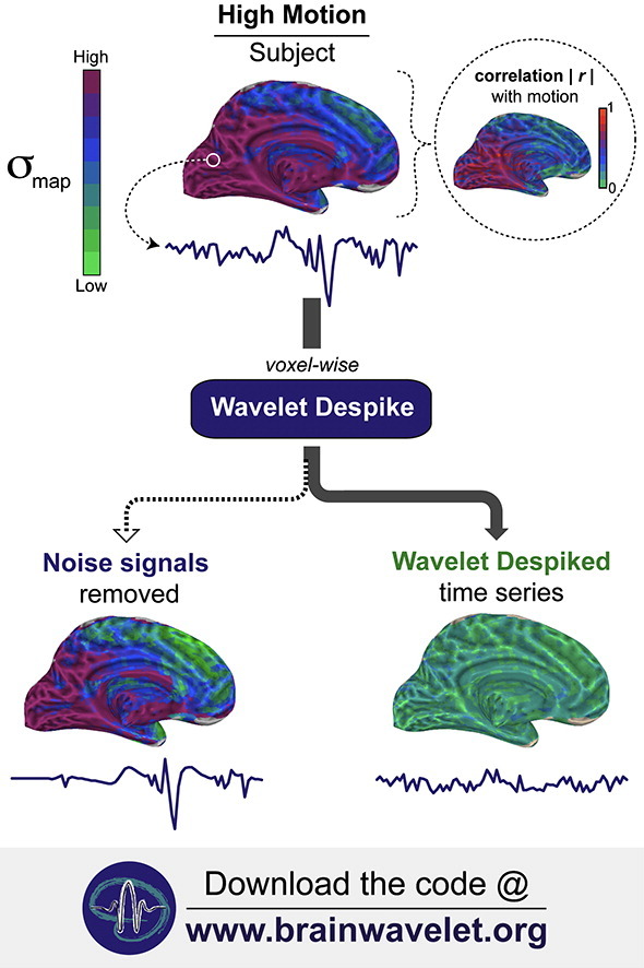
Fig. 1.

Overview of image and time series processing methods. This figure summarizes the key pre-processing steps used to process the resting-state fMRI data. Pre-processing was divided into core image processing, and denoising. *Fourier filtering was restricted to a high-pass filter (0.009 Hz < f), except for the analyses presented in Inline Supplementary Figs. S1, S5, S6 and S7, where a band-pass filter (0.009 < f < 0.08 Hz) was used. Results in Figs. 3, 5, and 6, and Inline Supplementary Fig. S4, which show outputs immediately after despiking, do not include any frequency filtering. A more detailed diagram of our pre-processing methods can be found in Inline Supplementary Fig. S2.

Overview of image and time series processing methods. This figure summarizes the key pre-processing steps used to process the resting-state fMRI data. Pre-processing was divided into core image processing, and denoising. *Fourier filtering was restricted to a high-pass filter (0.009 Hz < f), except for the analyses presented in Inline Supplementary Figs. S1, S5, S6 and S7, where a band-pass filter (0.009 < f < 0.08 Hz) was used. Results in Figs. 3, 5, and 6, and Inline Supplementary Fig. S4, which show outputs immediately after despiking, do not include any frequency filtering. A more detailed diagram of our pre-processing methods can be found in Inline Supplementary Fig. S2.

Fig. S2.

Full image and time series processing pipeline. This figure highlights the key pre-processing steps, in the order they were implemented. Pre-processing was divided into two sections: core image processing, and denoising. *Fourier filtering was restricted to a high-pass filter (0.009 Hz < f), except for the analyses presented in Inline Supplementary Figs. S1, S5, S6 and S7, where a band-pass filter (0.009 < f < 0.08 Hz) was used. Results in Figs. 3, 5, 6, and Inline Supplementary Fig. S4, which show outputs immediately after despiking, do not include any frequency filtering.

Full image and time series processing pipeline. This figure highlights the key pre-processing steps, in the order they were implemented. Pre-processing was divided into two sections: core image processing, and denoising. *Fourier filtering was restricted to a high-pass filter (0.009 Hz < f), except for the analyses presented in Inline Supplementary Figs. S1, S5, S6 and S7, where a band-pass filter (0.009 < f < 0.08 Hz) was used. Results in Figs. 3, 5, 6, and Inline Supplementary Fig. S4, which show outputs immediately after despiking, do not include any frequency filtering.

Denoising steps included: (vii) time series despiking (wavelet or time domain); (viii) confound signal regression including the 6 motion parameters estimated in (ii), their first order temporal derivatives, and ventricular cerebrospinal fluid (CSF) signal (referred to as 13-parameter regression); and (ix) a temporal Fourier filter. Frequency filtering was restricted to a high-pass filter (0.009 Hz < f), except for the analyses presented in Inline Supplementary Figs. S1, S5, S6 and S7, in order to prevent temporal smoothing from biasing our inter-method comparisons. For these Supplementary figures, a temporal band-pass filter (0.009 < f < 0.08 Hz; frequency bands as in Power et al.. 2012) was applied in the final step, in order to facilitate comparison with results presented in Power et al. (2012) and Satterthwaite et al. (2012). Results in Figs. 3, 5, 6, and Inline Supplementary Fig. S4, which show outputs immediately after despiking, do not include any frequency filtering. We did not regress white matter or global signals, as they were found to increase distance-dependent connectivity biases in accordance with previously published reports (Satterthwaite et al., 2013; Jo et al., 2013; see Inline Supplementary Fig. S1). A summary of our pre-processing steps can be found in Fig. 1, and a more detailed overview in Inline Supplementary Fig. S2.

Inline Supplementary Figs. S1 and S2 can be found online at http://dx.doi.org/10.1016/j.neuroimage.2014.03.012.

Despiking algorithms

Two despiking algorithms were used for the analysis presented: the Wavelet Despiking algorithm was compared against a more standard type of despiking algorithm, here called the Time Despike. Both were implemented at a voxel level prior to confound signal regression.

Time Despike

This algorithm was implemented as part of AFNI's 3dBandpass function. This function identifies spikes as supra-threshold deviations from the local Median Absolute Deviation (MAD), and compresses these to the level of the local median. The following steps were conducted:

• 1.
  For each time series X_t, the local median was calculated at each time point from a local sample of 4 time points either side of any given time point (see Inline Supplementary Fig. S3A). So, for t = {4, …, N − 5}, where N is the number of time points,

  $${\mathrm{MED}}_{\mathit{t}}=\mathit{median}\left(\left\{{\mathit{X}}_{\mathit{t}-4},\dots ,{\mathit{X}}_{\mathit{t}+4}\right\}\right).$$ (1)
  For each time series X_t, the local median was calculated at each time point from a local sample of 4 time points either side of any given time point (see Inline Supplementary Fig. S3A). So, for t = {4, …, N − 5}, where N is the number of time points,

  $${\mathrm{MED}}_{\mathit{t}}=\mathit{median}\left(\left\{{\mathit{X}}_{\mathit{t}-4},\dots ,{\mathit{X}}_{\mathit{t}+4}\right\}\right).$$ (1)

  Inline Supplementary Figure S3.

  Inline Supplementary Fig. S3 can be found online at http://dx.doi.org/10.1016/j.neuroimage.2014.03.012.

  This window was compressed at the time series boundaries for t = {0, …, 3, N − 4, …, N − 1}, so for example,

  $${\mathrm{MED}}_0=\mathit{median}\left(\left\{{\mathit{X}}_0,\dots ,{\mathit{X}}_4\right\}\right).$$ (2)
• 2.
  For each time point, the local MAD was then calculated as follows, again within a 4 × 4 window (see Inline Supplementary Fig. S3B): for t = {4, …, N − 5}

  $$\begin{array}{l}{\mathrm{MAD}}_{\mathit{t}}=\mathit{median}\left(\left\{\left|{\mathit{X}}_{\mathit{t}-4}-{\mathrm{MED}}_{\mathit{t}}\right|,\dots \right)\right)\\ \left(\left(\left|{\mathit{X}}_{\mathit{t}+4}-{\mathrm{MED}}_{\mathit{t}}\right|\right\}\right).\end{array}$$ (3)
  For each time point, the local MAD was then calculated as follows, again within a 4 × 4 window (see Inline Supplementary Fig. S3B): for t = {4, …, N − 5},

  $$\begin{array}{l}{\mathrm{MAD}}_{\mathit{t}}=\mathit{median}\left(\left\{\left|{\mathit{X}}_{\mathit{t}-4}-{\mathrm{MED}}_{\mathit{t}}\right|,\dots \right)\right)\\ \left(\left(\left|{\mathit{X}}_{\mathit{t}+4}-{\mathrm{MED}}_{\mathit{t}}\right|\right\}\right).\end{array}$$ (3)
  Again, the window was compressed at the time series boundaries for t = {0, …, 3, N − 4, …, N − 1}, so for example,

  $$\begin{array}{l}{\mathrm{MAD}}_1=\mathit{median}\left(\right\{\left|{\mathit{X}}_0-{\mathrm{MED}}_1\right|,\dots ,\\ \left|{\mathit{X}}_5-{\mathrm{MED}}_1\right|\left\}\right).\end{array}$$ (4)
• 3.
  For each time point, if the time point's deviation from the local median was greater than the MAD for that time point × 6.8, then that time point was despiked to the level of the local median (see Inline Supplementary Fig. S3C). So, for t = {0, …, N − 1},

  $$\begin{array}{l}\mathrm{if}\left|{\mathit{X}}_{\mathit{t}}-{\mathrm{MED}}_{\mathit{t}}\right|>{\mathrm{MAD}}_{\mathit{t}}\times 6.8\\ \mathrm{then}{\mathit{X}}_{\mathit{t}}={\mathrm{MED}}_{\mathit{t}}.\end{array}$$ (5)
  For each time point, if the time point's deviation from the local median was greater than the MAD for that time point × 6.8, then that time point was despiked to the level of the local median (see Inline Supplementary Fig. S3C). So, for t = {0, …, N − 1},

  $$\begin{array}{l}\mathrm{if}\left|{\mathit{X}}_{\mathit{t}}-{\mathrm{MED}}_{\mathit{t}}\right|>{\mathrm{MAD}}_{\mathit{t}}\times 6.8\\ \mathrm{then}{\mathit{X}}_{\mathit{t}}={\mathrm{MED}}_{\mathit{t}}.\end{array}$$ (5)

Fig. S3.

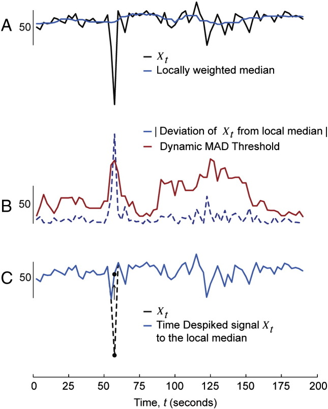
Guided example of the Time Despike method. For each time point in time series X_t, the local median was first calculated from a local region (4 × 4 window) of values in the neighborhood of that time point (A). The local Median Absolute Deviation (MAD) was then calculated for each time point across this same window (B). Any time point that had a larger value than the MAD multiplied by a threshold value of 6.8, was despiked to the level of the local median (C). Please see the Time Despike section for more details.

Wavelet Despike

This algorithm was designed to identify non-stationary events caused by motion, using a wavelet-based approach. Wavelet analysis offers a powerful set of tools for analyzing the properties of complex time series (Daubechies, 1992; Mallat, 1998). Wavelet transforms provide multi-resolution (multi-frequency) information about signals, and are known to be effective at detecting transient phenomena, such as spikes, for which Fourier methods are relatively ineffective (Mallat, 1998).

The Wavelet Despiking algorithm comprised five key steps, which are detailed below. A diagrammatic explanation of these steps can be found in Fig. 2.

• 1.
  Time series decomposition. Each voxel time series X_t was decomposed in the wavelet domain to ${\displaystyle {\tilde{\mathit{W}}}_{\mathit{s},\mathit{t}}}$, using the (partial) Maximal Overlap Discrete Wavelet Transform (MODWT, WMTSA toolbox: http://www.atmos.washington.edu/wmtsa/); s represents the scale, or frequency band, and t represents time, where s = {1, …, J}, t = {0, …, N − 1}, J is the number of scales, and N is the number of time points. J was defined as the largest positive integer satisfying the condition:

  $$\mathit{J}\le \mathit{lo}{\mathit{g}}_2\left(\mathit{N}\right)\mathrm{where}\mathit{J}\in {\mathrm{\mathbb{Z}}}^{+}.$$ (6)

  The MODWT was implemented using the pyramid algorithm (Percival and Walden, 2006), and Daubechies scaling (father) and wavelet (mother) filters of length 4 (db4; Daubechies, 1992). The MODWT has a number of key advantages over the Discrete Wavelet Transform (DWT), which makes it particularly useful for our purposes. First, it is naturally defined for all sample sizes. Thus, the length of time series has no ‘power of 2’ restrictions. In addition, the MODWT can eliminate alignment artifacts (Percival and Walden, 2006), making it easier to detect transients in coarser scales that are due to an event at a particular point in time.

  For N time points, the MODWT wavelet $\left(\tilde{\mathit{W}}\right)$ and scaling $\left(\tilde{\mathit{V}}\right)$ coefficients of signal X_t were defined as follows:

  $$\begin{array}{l}\mathrm{for}\mathit{t}=\left\{0,\dots ,\mathit{N}-1\right\}\mathrm{and}\mathit{s}=\left\{1,\dots ,\mathit{J}\right\}\\ {\displaystyle {\tilde{\mathit{W}}}_{\mathit{s},\mathit{t}}}\equiv {\displaystyle \sum _{\mathit{l}=0}^{{\mathit{L}}_{\mathit{s}}-1}{\displaystyle {\tilde{\mathit{h}}}_{\mathit{s},\mathit{l}}}}\cdot {\mathit{X}}_{\mathit{t}-\mathit{lmodN}}\&\\ {\displaystyle {\tilde{\mathit{V}}}_{\mathit{s},\mathit{t}}}\equiv {\displaystyle \sum _{\mathit{l}=0}^{{\mathit{L}}_{\mathit{s}}-1}{\displaystyle {\tilde{\mathit{g}}}_{\mathit{s},\mathit{l}}}}\cdot {\mathit{X}}_{\mathit{t}-\mathit{lmodN}}\\ \mathrm{where}\left\{{\displaystyle {\tilde{\mathit{h}}}_{\mathit{s},\mathit{l}}}:\mathit{l}=0,\dots ,{\mathit{L}}_{\mathit{s}}-1\right\}\&\\ \left\{{\displaystyle {\tilde{\mathit{g}}}_{\mathit{s},\mathit{l}}}:\mathit{l}=0,\dots ,{\mathit{L}}_{\mathit{s}}-1\right\}.\end{array}$$ (7)

  The MODWT wavelet and scaling filters (${\displaystyle {\tilde{\mathit{h}}}_{\mathit{s},\mathit{l}}}$ and ${\displaystyle {\tilde{\mathit{g}}}_{\mathit{s},\mathit{l}}}$ respectively) have length (2^S − 1)(L − 1) + 1.

  The pyramid algorithm (Percival and Walden, 2006) computes scale s wavelet $\left(\tilde{\mathit{W}}\right)$ and scaling $\left(\tilde{\mathit{V}}\right)$ coefficients from scale s − 1 scaling coefficients $\left({\displaystyle {\tilde{\mathit{V}}}_{\mathit{s}-1}}\right)$ as follows:

  $$\begin{array}{l}\mathrm{letting}{\displaystyle {\tilde{\mathit{V}}}_{0,\mathit{t}}}\equiv {\mathit{X}}_{\mathit{t}}\mathrm{for}\mathrm{all}\mathit{s}\ge 1\\ {\displaystyle {\tilde{\mathit{W}}}_{\mathit{s},\mathit{t}}}={\displaystyle \sum _{\mathit{l}=0}^{\mathit{L}-1}{\displaystyle {\tilde{\mathit{h}}}_{\mathit{l}}}}\cdot {\displaystyle {\tilde{\mathit{V}}}_{\mathit{s}-1,\mathit{t}-2^{\mathit{s}-1}\mathit{lmodN}}}\&\\ {\displaystyle {\tilde{\mathit{V}}}_{\mathit{s},\mathit{t}}}={\displaystyle \sum _{\mathit{l}=0}^{\mathit{L}-1}{\displaystyle {\tilde{\mathit{g}}}_{\mathit{l}}}}\cdot {\displaystyle {\tilde{\mathit{V}}}_{\mathit{s}-1,\mathit{t}-2^{\mathit{s}-1}\mathit{lmodN}}}.\end{array}$$ (8)
  Next, coefficients at each scale were temporally aligned according to the phase delay properties of the filter applied. For the db4 filter, the circular shift is defined at each scale by T_s, which is calculated as follows: for s = {1 …, J}, and where L = 4 (the filter length),

  $${\mathit{T}}_{\mathit{s}}=2^{\mathit{s}-1}\left(\mathit{L}-1\right)-1.$$ (9)
  Thus, all wavelet coefficients ${\displaystyle {\tilde{\mathit{W}}}_{\mathit{s},\mathit{t}}}$ were redefined as follows:

  $${\displaystyle {\tilde{\mathit{W}}}_{\mathit{s},\mathit{t}}}={\displaystyle {\tilde{\mathit{W}}}_{\mathit{s},\mathit{t}-{\mathit{T}}_{\mathit{s}}}}.$$ (10)
• 2.Definition of maximal and minimal wavelet coefficients. After temporal alignment, the 2 × 2 neighborhood of each coefficient was searched for maximal or minimal wavelet coefficients, in the scale plane. Maxima and minima were considered separately throughout all steps, in order to preserve the directionality of the wavelet coefficients. This aided separation of non-stationary events where they occurred with relatively high frequency (continuously or in every few frames). This is an adaptation of the ‘modulus maxima method’, which is better suited for identifying non-stationary events which are rarer. One potential drawback of these methods is the limited temporal resolution, i.e. for a 2 × 2 neighborhood, a maximum or minimum can only be defined at most every 3 frames. This is a problem for identifying non-stationary events in all scales, but particularly for correctly identifying prolonged non-stationary events in higher scales (lower frequencies), such as low frequency artifacts, or spin-history type effects as spins realign after a large movement, and signal intensity slowly recovers. Therefore, to overcome these limitations in temporal resolution, a coefficient was defined as maximal (or minimal) if its value was at least half the size of the local maximum (or minimum). Details can be found below in Eqs. (11)–(13).
  For s = {1, …, J} and t = {2, …, N − 3}, the set of maxima ${\displaystyle {\tilde{\mathit{W}}}_{\mathit{max}}}$, and minima ${\displaystyle {\tilde{\mathit{W}}}_{\mathit{min}}}$ was defined as any set of wavelet coefficients, ${\displaystyle {\tilde{\mathit{W}}}_{\mathit{s},\mathit{t}}}$, that satisfied the following conditions:

  $$\begin{array}{l}{\displaystyle {\tilde{\mathit{W}}}_{\mathit{max}}}\equiv \left\{{\displaystyle {\tilde{\mathit{W}}}_{\mathit{s},\mathit{t}}}\ge 0.5\cdot \mathit{max}\left(\left\{{\displaystyle {\tilde{\mathit{W}}}_{\mathit{s},\mathit{t}-2}},\dots ,{\displaystyle {\tilde{\mathit{W}}}_{\mathit{s},\mathit{t}+2}}\right\}\right)\right\}\&\\ {\displaystyle {\tilde{\mathit{W}}}_{\mathit{min}}}\equiv \left\{{\displaystyle {\tilde{\mathit{W}}}_{\mathit{s},\mathit{t}}}\le 0.5\cdot \mathit{min}\left(\left\{{\displaystyle {\tilde{\mathit{W}}}_{\mathit{s},\mathit{t}-2}},\dots ,{\displaystyle {\tilde{\mathit{W}}}_{\mathit{s},\mathit{t}+2}}\right\}\right)\right\}.\end{array}$$ (11)
  Function boundaries for t were circularized for each scale, such that for t = {0, 1, N − 2, N − 1} and s = {1, …, J}, the wavelet coefficient ${\displaystyle {\tilde{\mathit{W}}}_{\mathit{s},\mathit{N}-1}}$ was considered maximal if:

  $$\begin{array}{l}{\displaystyle {\tilde{\mathit{W}}}_{\mathit{s},\mathit{N}-1}}\ge 0.5\cdot \mathit{max}\left(\left\{{\displaystyle {\tilde{\mathit{W}}}_{\mathit{s},\mathit{N}-3}},\dots ,{\displaystyle {\tilde{\mathit{W}}}_{\mathit{s},\mathit{N}-1}}\right)\right)\\ \left(\left({\displaystyle {\tilde{\mathit{W}}}_{\mathit{s},0}},{\displaystyle {\tilde{\mathit{W}}}_{\mathit{s},1}}\right\}\right)\end{array}$$ (12)

  and minimal if:

  $$\begin{array}{l}{\displaystyle {\tilde{\mathit{W}}}_{\mathit{s},\mathit{N}-1}}\le 0.5\cdot \mathit{min}\left(\left\{{\displaystyle {\tilde{\mathit{W}}}_{\mathit{s},\mathit{N}-3}},\dots ,{\displaystyle {\tilde{\mathit{W}}}_{\mathit{s},\mathit{N}-1}}\right)\right)\\ \left(\left({\displaystyle {\tilde{\mathit{W}}}_{\mathit{s},0}},{\displaystyle {\tilde{\mathit{W}}}_{\mathit{s},1}}\right\}\right).\end{array}$$ (13)
  This produced a relatively dense set of maximal and minimal wavelet coefficients. In order to identify which coefficients in ${\displaystyle {\tilde{\mathit{W}}}_{\mathit{max}}}$ and ${\displaystyle {\tilde{\mathit{W}}}_{\mathit{min}}}$ originated from large non-stationary events, we used the common method, within the modulus maxima method literature, of thresholding coefficients. We used a lenient threshold, which retained many of these coefficients, as we subsequently used a chain detection algorithm to identify large non-stationary events crossing multiple scales or frequency bands. The sets of maximal and minimal wavelet coefficients surviving the thresholding operation, denoted ${\displaystyle {\tilde{\mathit{W}}}_{\mathit{max}}}$ and ${\displaystyle {\tilde{\mathit{W}}}_{\mathit{min}}}$ respectively, were thus defined as follows:

  $$\begin{array}{l}{\tilde{\mathit{W}}}_{\mathit{max}}^{\prime }\equiv \left\{{\displaystyle {\tilde{\mathit{W}}}_{\mathit{max}}}|{\displaystyle {\tilde{\mathit{W}}}_{\mathit{max}}}\in {\mathrm{\mathbb{Z}}}^{\ge 10}\right\}\&\\ {\tilde{\mathit{W}}}_{\mathit{min}}^{\prime }\equiv \left\{{\displaystyle {\tilde{\mathit{W}}}_{\mathit{min}}}|{\displaystyle {\tilde{\mathit{W}}}_{\mathit{min}}}\in {\mathrm{\mathbb{Z}}}^{\le -10}\right\}.\end{array}$$ (14)
• 3.
  Maxima and minima chain search algorithm. Non-stationary events caused by abrupt changes in time series are represented as chains of maximal and minimal wavelet coefficients, present at the same time point, but in multiple scales or frequencies. These chains characterize both the higher and lower frequency time series components related to the abrupt non-stationary change. To prove mathematically which maxima or minima propagate from lower to higher scales, we would need a very large set of scales, which is computationally expensive. A commonly used approximation is to implement a search algorithm that looks at the position and directionality of the maximal or minimal coefficient at any given scale relative to other maxima or minima in the same, or adjacent, scales. So, for example, a coefficient in the set ${\displaystyle {\tilde{\mathit{W}}}_{\mathit{max}}}$ at s = 1 will be chained to a coefficient at s = 2, if it is of the same sign, and its position is close (within two time points and one scale) to the coefficient at s = 1. Sets of coefficients ${\tilde{\mathit{W}}}_{\mathit{max}}^{\prime }$, and ${\displaystyle {\tilde{\mathit{W}}}_{\mathit{min}}^{\prime }}$ were thus entered into the search algorithm independently. Taking the example of ${\tilde{\mathit{W}}}_{\mathit{max}}^{\prime }$, coefficients that were part of maxima chains ${\displaystyle {\tilde{\mathit{W}}}_{\mathit{Cmax}}^{\prime }}$, were defined as follows: for s = {2, …, J − 1}, and t = {2, …, N − 3},

  $$\begin{array}{l}{\displaystyle {\tilde{\mathit{W}}}_{\mathit{Cmax}}}\subseteq {\tilde{\mathit{W}}}_{\mathit{max}}^{\prime },\mathrm{such}\mathrm{that}\\ {\displaystyle {\tilde{\mathit{W}}}_{\mathit{Cmax}}}\equiv \left\{{\tilde{\mathit{W}}}_{\mathit{max}}^{\prime }|{\displaystyle {\tilde{\mathit{W}}}_{\mathit{s}+\mathit{k},\mathit{t}+\mathit{l}}}\in {\tilde{\mathit{W}}}_{\mathit{max}}^{\prime }\right\},\\ \mathrm{for}\mathrm{any}\mathrm{value}\mathrm{of}\mathit{k}\in \left\{-1,0,1\right\}\mathrm{and}\mathit{l}\in \left\{-2,\dots ,2\right\},\\ \mathrm{but}\mathrm{where}\left(\mathit{k},\mathit{l}\right)\ne \left(0,0\right).\end{array}$$ (15)

  The same conditions were applied to ${\tilde{\mathit{W}}}_{\mathit{min}}^{\prime }$, to produce a set of minima chains, ${\displaystyle {\tilde{\mathit{W}}}_{\mathit{Cmin}}}$. We refer to this final set of coefficients comprising maxima, ${\displaystyle {\tilde{\mathit{W}}}_{\mathit{Cmax}}}$, and minima, ${\displaystyle {\tilde{\mathit{W}}}_{\mathit{Cmin}}}$, chains as ${\displaystyle {\tilde{\mathit{W}}}_{\mathit{MMC}}}$ (i.e. ${\displaystyle {\tilde{\mathit{W}}}_{\mathit{MMC}}}=\left\{{\displaystyle {\tilde{\mathit{W}}}_{\mathit{Cmax}}},{\displaystyle {\tilde{\mathit{W}}}_{\mathit{Cmin}}}\right\}$). Boundaries were circularized in the time dimension, t, as in the previous step; so for example, where t = 0, the values t + l could take were: t + l ∈ {N − 2, N − 1, 0, 1, 2}.

• 4.
  Maxima and minima chain removal. All coefficients at position ${\displaystyle {\tilde{\mathit{W}}}_{\mathit{s},\mathit{t}}}$ that were part of maxima and minima chains, ${\displaystyle {\tilde{\mathit{W}}}_{\mathit{MMC}}}$, were then located and set to zero in the scale-time plane, $\forall {\displaystyle {\tilde{\mathit{W}}}_{\mathit{s},\mathit{t}}}\in {\displaystyle {\tilde{\mathit{W}}}_{\mathit{MMC}}}$, for s = {1, …, J} and t = {0, …, N − 1}. In other words, maxima and minima chains were masked out in the wavelet domain. All wavelet coefficients were then re-shifted back out of temporal alignment, according to the phase delay of the filter, before the signal was recomposed. The time shift function is given in Eq. (9) above. Wavelet coefficients ${\displaystyle {\tilde{\mathit{W}}}_{\mathit{s},\mathit{t}}}$ were thus redefined as follows:

  $${\displaystyle {\tilde{\mathit{W}}}_{\mathit{s},\mathit{t}}}={\displaystyle {\tilde{\mathit{W}}}_{\mathit{s},\mathit{t}+{\mathit{T}}_{\mathit{s}}}}.$$ (16)
• 5.
  Time series recomposition. After non-stationary events had been removed, the ‘Wavelet Despiked’ (denoised) signal could be recomposed from all scales using the inverse MODWT (iMODWT). This was done using the inverse pyramid algorithm (Percival and Walden, 2006):

  $${\displaystyle {\tilde{\mathit{V}}}_{\mathit{s}-1,\mathit{t}}}={\displaystyle \sum _{\mathit{l}=0}^{\mathit{L}-1}{\displaystyle {\tilde{\mathit{h}}}_{\mathit{l}}}}\cdot {\displaystyle {\tilde{\mathit{W}}}_{\mathit{s},\mathit{t}+2^{\mathit{s}-1}\mathit{lmod}\mathit{N}}}+{\displaystyle \sum _{\mathit{l}=0}^{\mathit{L}-1}{\displaystyle {\tilde{\mathit{g}}}_{\mathit{l}}}}\cdot {\displaystyle {\tilde{\mathit{V}}}_{\mathit{s},\mathit{t}+2^{\mathit{s}-1}\mathit{lmod}\mathit{N}}}.$$ (17)

  For some analyses, the final set of maxima and minima chain coefficients themselves was recomposed to create a ‘noise signal’. In this case, all wavelet coefficients not part of the set of maxima or minima chains, ${\displaystyle {\tilde{\mathit{W}}}_{\mathit{s},\mathit{t}}}\notin {\displaystyle {\tilde{\mathit{W}}}_{\mathit{MMC}}},\mathrm{for}\mathit{s}=\left\{1,\dots ,\mathit{J}\right\}\mathrm{and}\mathit{t}=\left\{0,\dots ,\mathit{N}-1\right\}$, were set to zero in the scale-time plane, and the noise signal recomposed from all scales using the iMODWT.

  Where frequency filtering was conducted, despiked, and recomposed, time series were filtered in the Fourier domain (following regression) in order to keep frequency bands consistent with the Time Despiking method. We note that it is also possible to frequency filter in the wavelet domain by recomposing a subset of scales, or indeed to use the wavelet coefficients themselves for connectivity analysis.

Fig. 2.

Guided example of the Wavelet Despike method. Each numbered step in the figure refers to the correspondingly numbered step in the Wavelet Despike section. Wavelet Despiking was performed for each voxel time series separately. In step (1), each time series was decomposed using the Maximal Overlap Discrete Wavelet Transform (MODWT) to add an extra dimension of information, the scale (or frequency band). The wavelet decomposition is represented as a number matrix of time vs. scale (or frequency band). In (2), local maxima and minima were defined from this matrix by searching through coefficients in the scale plane. For each coefficient, maxima and minima were defined within a local 2 × 2 window of coefficients, and boundaries were circularized. A coefficient was defined as maximal (or minimal) if its value was at least half the size of the local (within a 2 × 2 window) maximum (or minimum) and its modulus was greater than a threshold value of 10. This produced a relatively dense set of maxima and minima; the diagram only shows a few of these for clarity. In step (3), maxima and minima were chained across scales. For each maximum, a sliding window function searched across scales for any adjacent maxima (denoted in pink), and for each minimum, searched for adjacent minima (denoted in blue). The window size was fixed at 2 × 2 in the scale plane, 1 × 1 in the time plane, and was circularized in the scale plane. Only maxima that had at least one other accompanying maximum within this window were kept (denoted by ticks), others were removed from the set (denoted by crosses); the same applied for the set of minima. This resulted in a final set of maximal and minimal wavelet coefficients that were part of maxima or minima chains. In the final step (4), the signals were recomposed using the inverse Maximal Overlap Discrete Wavelet Transform (iMODWT). Two time series were recomposed at this stage. First, the set of maximal and minimal wavelet coefficients were removed from the time vs scale plane, and the remaining coefficients recomposed to create a denoised ‘Wavelet Despiked’ time series. Secondly, the maximal and minimal wavelet coefficients themselves were recomposed to create a ‘noise signal’. The noise signals were used for a variety of analyses to look at the nature of the signals being removed by the algorithm.

Definition of regional time series

After functional image pre-processing, voxel time series were parcellated into 230 approximately evenly-sized parcels. The template was made by randomly parcellating gray matter regions (Zalesky et al., 2010) as identified by the Eickhoff–Zilles macrolabels atlas in Talairach space (distributed with AFNI). Voxel time series within each parcel were averaged to form regional time series. The template was created to contain a comparable number of parcels to those described in Power et al. (2012) and Satterthwaite et al. (2012), which used 264 and 160 regions of interest, respectively.

To ensure that our results were template independent, we repeated our core analyses with two additional templates: another randomly parcellated gray matter template comprising 325 parcels; and an anatomical parcellation, based on the Eickhoff–Zilles atlas in Talairach space, comprising 116 parcels. The use of these alternate templates did not change our findings.

Framewise Displacement, DVARS and Spike Percentage

Movement was quantified and summarized into a single vector for each subject using four different methods; including three previously published measures: Framewise Displacement (FD; Power et al., 2012), root mean square displacement (rmsFD; Satterthwaite et al., 2012, 2013), DVARS (Smyser et al., 2010; Power et al., 2012), and Spike Percentage (new).

Framewise Displacement

Framewise Displacement (FD) was defined as the sum of the absolute derivatives of the 6 motion parameters (x, y, z, α, β, γ), representing 3 planes of translation and 3 planes of rotation. Rotational parameters (yaw α, pitch β and roll γ) were converted to distances by computing the arc length displacement on the surface of a sphere with radius 50 mm (as in Power et al., 2012). For t = {1, …, N − 1}, where N = the number of time points.

$$\begin{array}{l}\mathit{F}{\mathit{D}}_{\mathit{t}}={\displaystyle \sum _{\mathit{d}\in \mathit{D}}\left|{\mathit{d}}_{\left(\mathit{t}-1\right)}-{\mathit{d}}_{\mathit{t}}\right|}+50\cdot \frac{\mathit{\pi }}{180}\cdot {\displaystyle \sum _{\mathit{r}\in \mathit{R}}\left|{\mathit{r}}_{\left(\mathit{t}-1\right)}-{\mathit{r}}_{\mathit{t}}\right|}\\ \mathrm{where}\mathit{D}=\left\{\mathit{x},\mathit{y},\mathit{z}\right\}\&\mathit{R}=\left\{\mathit{\alpha },\mathit{\beta },\mathit{\gamma }\right\}\end{array}$$ (18)

FD at time t = 0 was given the value 0 in order for the length of FD to equal N. For any subject $\overline{\mathit{FD}}$ was defined as the mean value of the FD vector.

Root mean square displacement

rmsFD was defined as the root mean square variance across the absolute frame-to-frame difference of the unaltered 6 movement parameters. Rotations were not converted to distances (as in Satterthwaite et al., 2012, 2013). For t = {1, …, N − 1},

$$\begin{array}{l}\mathit{rmsF}{\mathit{D}}_{\mathit{t}}=\sqrt{\frac{1}{6}\cdot {\displaystyle \sum _{\mathit{p}\in \mathit{P}}〈{\left|{\mathit{m}}_{\mathit{p}\left(\mathit{t}-1\right)}-{\mathit{m}}_{\mathit{pt}}\right|}^2〉}}\\ \mathrm{where}\mathit{P}=\left\{\mathit{x},\mathit{y},\mathit{z},\mathit{\alpha },\mathit{\beta },\mathit{\gamma }\right\}\end{array}$$ (19)

rmsFD at time t = 0 was given the value 0 in order for the length of rmsFD to equal N.

DVARS

DVARS, is the root mean square variance across all brain voxels, of frame-to-frame difference in percent signal change. DVARS was calculated at different stages within the denoising section of our functional image pre-processing pipeline, but before frequency filtering (see Fig. 1, Inline Supplementary Fig. S2), in order to analyze the effects of different operations on percent signal change. The stage of pre-processing after which DVARS was calculated, is indicated in the text and figure legends where relevant. For t = {1, …, N − 1},

$$\mathit{DV}\mathit{AR}{\mathit{S}}_{\mathit{t}}=\sqrt{\frac{1}{\mathit{n}\left(\mathit{V}\right)}\cdot {\displaystyle \sum _{\mathit{I}\in \mathit{V}}〈{\left[{\mathit{I}}_{\mathit{t}}-{\mathit{I}}_{\mathit{t}-1}\right]}^2〉}}$$ (20)

where V is the set of all voxel time series.

DVARS, is the root mean square variance across all brain voxels, of frame-to-frame difference in percent signal change. DVARS was calculated at different stages within the denoising section of our functional image pre-processing pipeline, but before frequency filtering (see Fig. 1, Inline Supplementary Fig. S2), in order to analyze the effects of different operations on percent signal change. The stage of pre-processing after which DVARS was calculated, is indicated in the text and figure legends where relevant. For t = {1, …, N − 1},

$$\mathit{DVAR}{\mathit{S}}_{\mathit{t}}=\sqrt{\frac{1}{\mathit{n}\left(\mathit{V}\right)}\cdot {\displaystyle \sum _{\mathit{I}\in \mathit{V}}〈{\left[{\mathit{I}}_{\mathit{t}}-{\mathit{I}}_{\mathit{t}-1}\right]}^2〉}}$$ (20)

where V is the set of all voxel time series.

DVARS at time t = 0 was given the value 0 in order for the length of DVARS to equal N.

Spike Percentage

The Spike Percentage (SP) at any given time point, is defined as the percentage of gray matter voxels containing a spike in that frame of data. For a run of N time points, the SP is therefore a vector of N points. Spikes may be defined in a number of ways, such as deviations above a threshold, or from the mean; but here we mark a time point for any given voxel time series as a spike, if there is a maximal or minimal wavelet coefficient (in the final set comprising maxima and minima chains) at that time point in scale s = 1 (see the Wavelet Despike section). In other words, the Spike Percentage for any given frame represents the percentage of gray matter voxels containing a maximal or minimal wavelet coefficient in scale s = 1 at that point in time. So, for t = {0, …, N − 1},

$$\mathit{S}{\mathit{P}}_{\mathit{t}}=\frac{\mathit{n}\left({\mathit{P}}_{\mathit{t}}\right)}{\mathit{G}}\times 100,{\mathit{P}}_{\mathit{t}}=\left\{{\displaystyle {\tilde{\mathit{W}}}_{1,\mathit{t}}}\in \mathit{C}\right\},$$ (21)

where G is the number of gray matter voxels, and C is the set of maxima and minima chain wavelet coefficients $\left({\displaystyle {\tilde{\mathit{W}}}_{\mathit{MMC}}}\right)$ across all gray matter voxels.

Unless otherwise indicated, the Spike Percentage was calculated after core image processing, and prior to any frequency filtering. For any subject, $\overline{\mathit{SP}}$ is the mean value of the SP vector.

Distance-dependent movement artifact diagnostics

Distance-dependent movement artifacts were analyzed in two ways, using two previously published group-level metrics: the ‘ΔR plot’ (which can also be computed at a single-subject level; Power et al., 2012), and the ‘motion correlation plot’ (Satterthwaite et al., 2012).

For each subject, the ΔR plot first requires the identification of motion-affected frames of data using the global measures of FD and DVARS. For these plots, DVARS was calculated immediately after core image processing (see Fig. 1). Marked frames were then scrubbed from all time series, after parcellation. The difference in correlation between pair-wise regional time series (scrubbed correlation minus unscrubbed correlation) was noted as ΔR. Frames were marked for removal if both the FD was > 0.5 mm (including 1 frame before and two frames after those marked, where possible) and DVARS was > 0.3% above baseline (similarly including 1 frame before and two frames after those marked). This DVARS threshold was chosen to be most similar to the fixed threshold of DVARS > 0.5% described in Power et al. (2012), but to also allow for variation in the baseline of DVARS, as occurs when different pre-processing strategies are employed. The more recently proposed criteria for scrubbing (Power et al., 2013; FD > 0.2 mm and DVARS > 0.3%) were not used here as they were found to remove excessive amounts of data (see Table 1). Group-level ΔR plots were made by computing ΔR for all 52,900 pair-wise correlations between the 230 regional time series, at a single-subject level, averaging the ΔR vectors across all subjects, and plotting ΔR as a function of the Euclidean distance between the centroids of these regions.

The motion-correlation plot (Satterthwaite et al., 2012) identifies whether pair-wise correlations between regional time series are correlated with motion, at a group level. To make this plot, we correlated an estimate of connectivity between each paired set of regional time series (determined by Pearson correlation between the two time series) with an estimate of that subject's motion, across all subjects. Motion here was defined by a single integer representing the mean absolute displacement relative to the previous frame, at each brain volume, averaged across x, y, and z planes (Satterthwaite et al., 2012). For each paired set of time series (52,900 in total), the correlation between motion and connectivity was plotted against the distance between the regions. This summarized whether group-level distance-dependent connectivity biases existed in the cohort as a whole.

Subject exclusion criteria

Subjects with a mean Spike Percentage $\left(\overline{\mathit{SP}}\right)$ > 5% were excluded from analysis. This included 6 subjects from cohort 1, 6 subjects from cohort 2, and 2 subjects from cohort 3. Compared to previously described criteria for exclusion, these subjects had, on average across the cohorts, < 0.1 min of good data, using FD >0.2 mm for identifying motion-affected frames (Yan et al., 2013); < 2.6 min of good data, using rmsFD >0.25 mm (Satterthwaite et al., 2013); and < 3.0 min of good data, using FD > 0.5 mm and ΔDVARS >0.3% (Power et al., 2012). This is in contrast to the 3, 4 and 5 min thresholds described in these papers respectively. Importantly, we do not consider all the frames marked as motion-affected by these methods as irrecoverable, and therefore we are able to keep considerably more datasets in high-motion cohorts (such as cohorts 1 and 2), than would be possible with any of the previously published methods.

A summary of the cohorts, including a comparison of the percentage of time points despiked by the Time and Wavelet Despiking methods, and different methods for scrubbing time series can be found in Table 1.

Results

Time series denoising capabilities of the Time and Wavelet Despike

We began by analyzing the ability of the despiking algorithms to identify and remove non-stationary events caused by movement, at a time series level. Cohort 1 subjects that had been pre-processed through the core image processing section of our pipeline (see Fig. 1) were entered into the Time and Wavelet Despike modules independently, and the outputs of the two were compared, along with the spikes or noise signals removed by the respective algorithms.

Example voxel time series from a moderately high and two lower motion cohort 1 subjects ($\overline{\mathit{S}}\mathit{P}$ = 2.7%, 1.0% and 0.5% respectively) can be found in Fig. 3, and further examples from two high-motion subjects ($\overline{\mathit{S}}\mathit{P}$ = 23.7%, 9.4% respectively) can be found in Inline Supplementary Fig. S4. The original signals represent time series that have just been processed through the core image processing module. In each case, spikes present in the original signals, that were coincident with subject movement, were effectively removed by the Wavelet Despike algorithm, but less efficiently by the Time Despike. Voxel time series were chosen to demonstrate a wide variety of motion artifacts, ranging from complex low frequency artifacts (Fig. 3, column 1), to high frequency artifacts combined with spin-history type effects, represented by a large drop in signal intensity taking many frames to recover (Fig. 3, column 2), to isolated ‘wide spikes’ caused by complex, isolated movements (Fig. 3, column 3), and finally, signal intensity changes resulting from multiple partial voxel shifts (Fig. 3, column 4). The Wavelet Despike algorithm was able to characterize and remove all of these artifacts from the fMRI time series, given that it characterizes events in multiple scales (frequency bands), thus enabling the removal of high frequency artifacts and any associated (or independent) lower frequency components. The Time Despike, a more standard procedure for despiking time series, was unsuccessful at removing many of these artifacts, because it uses a local median based method for identifying events in the time domain.

Example voxel time series from a moderately high and two lower motion cohort 1 subjects ($\overline{\mathit{SP}}$ = 2.7%, 1.0% and 0.5% respectively) can be found in Fig. 3, and further examples from two high-motion subjects ($\overline{\mathit{SP}}$ = 23.7%, 9.4% respectively) can be found in Inline Supplementary Fig. S4. The original signals represent time series that have just been processed through the core image processing module. In each case, spikes present in the original signals, that were coincident with subject movement, were effectively removed by the Wavelet Despike algorithm, but less efficiently by the Time Despike. Voxel time series were chosen to demonstrate a wide variety of motion artifacts, ranging from complex low frequency artifacts (Fig. 3, column 1), to high frequency artifacts combined with spin-history type effects, represented by a large drop in signal intensity taking many frames to recover (Fig. 3, column 2), to isolated ‘wide spikes’ caused by complex, isolated movements (Fig. 3, column 3), and finally, signal intensity changes resulting from multiple partial voxel shifts (Fig. 3, column 4). The Wavelet Despike algorithm was able to characterize and remove all of these artifacts from the fMRI time series, given that it characterizes events in multiple scales (frequency bands), thus enabling the removal of high frequency artifacts and any associated (or independent) lower frequency components. The Time Despike, a more standard procedure for despiking time series, was unsuccessful at removing many of these artifacts, because it uses a local median based method for identifying events in the time domain.

Inline Supplementary Fig. S4 can be found online at http://dx.doi.org/10.1016/j.neuroimage.2014.03.012.

Impact of despiking on time series correlation with movement and percent signal change

We next looked at the effects of the two despiking procedures on correlation between voxel time series and movement across the brain. Voxel time series from cohort 1 subjects were quantitatively compared, using Pearson correlation, with their respective Framewise Displacement and Spike Percentage vectors, under a number of pre-processing scenarios prior to frequency filtering, to produce two sets of correlation maps. Across all subjects, images that had only been processed through the core image processing module, contained considerable negative correlation with movement, due to the widespread presence of negatively deflecting spikes in the time series. An example from two high-movement subjects, one displaying globally correlated movement artifacts, and the other displaying locally correlated movement artifacts, can be found in Fig. 4 (subjects 1 and 2 respectively). Negative correlation with movement was reduced, but not eliminated, by the addition of 13-parameter regression (6 motion parameters, their first order temporal derivatives, and CSF signal; see Fig. 4A, row 2). However, the application of either the Time Despike or Wavelet Despike prior to 13-parameter regression produced significantly improved results, with near complete elimination of globally (subject 1) and locally (subject 2) correlated movement (see Fig. 4A, rows 3 and 4).

Fig. 4.

Effects of despiking on time series correlation with movement and percent signal change. (A) For two high-movement cohort 1 subjects, voxel time series were correlated with estimates of subject movement (Framewise Displacement) or the percentage of gray matter voxels containing spikes for each frame of data (Spike Percentage, see the Framewise Displacement, DVARS and Spike Percentage section of the Methods), under various pre-processing scenarios. Row 1 maps were generated immediately after core image processing (see Fig. 1). Row 2–4 map were generated under different pre-processing scenarios immediately after core image processing. In all cases, low-pass filtering was omitted. (B) DVARS traces for the subjects in (A). Upper panels show the effects of Time Despiking + 13-parameter regression (blue), and lower panels show the effects of Wavelet Despiking + 13-parameter regression (green). The DVARS trace for the noise signal removed by the Wavelet Despike algorithm is also shown for each subject (brown). In summary, despiking prior to regression was able to reduce time series correlation with movement better than regression alone, and large fluctuations in frame-to-frame percent signal change were captured and removed much more effectively by the Wavelet Despike than the Time Despike.

The ability of these despiking operations to suppress large frame-to-frame fluctuations in percent signal change (DVARS), caused by subject movement, in these high-movement subjects was then compared. Both the Time and Wavelet Despike algorithms were able to dampen large frame-to-frame fluctuations in DVARS; however, the Wavelet Despike produced considerably better results, with near complete suppression, and a resulting near-flat DVARS trace, without the application of a low-pass filter (Fig. 4B). These high-amplitude fluctuations were almost completely captured by the noise signal removed by this algorithm (Fig. 4B, row 2).

Spatial adaptivity of despiking

Given that the despiking algorithms despike all voxels independently, they have the flexibility of being spatially adaptive, that is, they can be tuned to remove motion artifacts only in voxels where they are present, in contrast to a global operation like scrubbing. In the case of the despiking algorithms we use, this tuning is unsupervised. To quantify the spatial heterogeneity of time series variance, and to investigate how the despiking algorithms deal for this, we analyzed standard deviation maps of cohort 1 subjects, before and after despiking. We used the standard deviation, as opposed to variance, in order to highlight the more subtle spatial effects of movement. As demonstrated by the high-movement example subject in Fig. 5, areas of high standard deviation (Fig. 5B) corresponded to areas of high correlation with movement (Fig. 5A), due to the presence of high-amplitude spikes in the time series. While the Time Despike was able to remove much of this motion-related signal variance, it did not perform nearly as well as the Wavelet Despike, which was able to more robustly capture signal variance related to movement. We observed this effect across all subjects analyzed. Further examples from a range of high-, medium- and low-motion cohort 1 subjects can be found in Fig. 6. Importantly, brain areas in the ‘noise signal removed’ maps (Figs. 5B and 6) with low standard deviation (green areas) were areas that were identified as ok by the Wavelet Despike algorithm, and therefore not despiked.

A comparison of despiking with previously published methods

A number of methods have been proposed to alleviate movement biases, including both scrubbing and regression techniques applied globally to all brain voxels. We first analyzed scrubbing with regard to the identification of spike-containing frames. Scrubbing uses the Framewise Displacement (FD) and/or DVARS to identify motion-affected frames, and censors these from time series. As we demonstrate in Figs. 7A and B, FD and DVARS do not always correctly identify spike-containing frames. We highlighted this by correlating these vectors with the Spike Percentage (SP) for all cohort 1 subjects (Fig. 7B). This latter measure is, by definition, sensitive to small subsets of voxels containing spikes (see the Framewise Displacement, DVARS and Spike Percentage section of the Methods), which may be enough to contribute a connectivity bias if spikes in these areas of the brain are not correctly identified and removed. We note that since the ‘ground truth’ in resting-state data is in fact unknown, the SP is simply an estimate of the noise introduced into fMRI time series by abrupt head movement. While FD and DVARS generally capture frames containing large artifacts, any thresholding operation on these vectors may miss more subtle biases (see Fig. 7A). In order to quantify this, we compared the ability of different scrubbing thresholds, proposed in different studies, to correctly identify spike-containing frames across all subjects in cohort 1. Masks of motion-affected frames identified by these methods were augmented with 1 frame before, and 2 frames after those marked, as described in Power et al. (2012). Here, we defined spike-containing frames as frames with a SP > 0.25%, as this corresponded to, on average, 125 voxels (the largest region size in our 230 region parcellation). The single criterion approach for scrubbing within regression (spike regression) of rmsFD > 0.25 mm (Satterthwaite et al., 2013), and the dual criteria approach for scrubbing of FD > 0.5 mm and ΔDVARS > 0.5% (Power et al., 2012), not only were the least aggressive, but also correctly identified on average fewer than 40 % of spike-containing frames (Fig. 7C, left panel). In contrast, the single criterion approach of FD >0.2 mm (Yan et al. 2013) and the dual criteria approach of FD >0.2 mm and ∆DVARS >0.3 % (Power et al., 2013) for scrubbing, both produced relatively good (> 75%) identification of spike-containing frames (Fig. 7C, left panel), but were considerably more aggressive, removing large numbers of frames (> 60% and > 80%, respectively; Fig. 7C, right panel). The Wavelet Despike method, by contrast, despiked on average 1.5% of time points from gray matter time series across the cohorts, without removing any frames of data. A summary of the percentage of time points that would be removed by the most recently proposed scrubbing methods, compared with the percentage of time points impacted by despiking, for all cohorts, can be found in Table 1.

Fig. 7.

Scrubbing methods do not always correctly identify spike-containing frames. (A) Framewise Displacement, DVARS and Spike Percentage vectors for a single subject in cohort 1 (see the Framewise Displacement, DVARS and Spike Percentage section of the Methods for information on how these vectors were computed). This demonstrates that frames containing spikes in small areas of the brain (identified by the Spike Percentage, shaded in gray) may not always be picked up by the global measures of Framewise Displacement and DVARS. The Spike Percentage was calculated after core image processing, and DVARS after 13-parameter regression and high-pass filtering at 0.009 Hz (as in Power et al., 2012). The low-pass filter was omitted here, to prevent bias from temporal smoothing. (B) The relationship between Spike Percentage and both Framewise Displacement and DVARS, across all subjects in cohort 1. Lines represent the linear best fit when the two vectors presented in the x and y axes were plotted against each other. Lines were extrapolated for some subjects in order to allow better visual comparison between subjects. While there is good correspondence for some subjects, this is not always the case, as highlighted by the group average correlation $\left({\displaystyle {\overline{\mathit{r}}}_{\mathit{group}}}\right)$. (C) Left panel shows the percentage of spike-containing frames captured by the different scrubbing criteria described in previous papers, across all subjects in cohort 1. Spike-containing frames were defined as any frame with a Spike Percentage > 0.25%. This corresponded to, on average, 125 voxels, which was the maximum size of any region defined by our 230 region parcellation. Outlier points marked by crosses are subjects with values > q₃ + 1.5(q₃ − q₁) or < q₁ − 1.5(q₃ − q₁), where q_n refers to the relevant quartile. Right panel shows the percentage of data left across all subjects in cohort 1 for the top three box plots in the left panel, compared to the percentage of spike-containing frames successfully identified.

We then directly compared previously published regression approaches, with the Time and Wavelet Despike algorithms proposed here. These included the Friston 24 autoregressive approach (Friston et al., 1996; 6 motion parameters, their square terms, and these 12 parameters modeled one frame back) described in Yan et al. (2013), and the higher-order motion parameter regression model (6 motion parameters + CSF signal, their first order temporal derivatives, and the square of these 14 parameters) described in Satterthwaite et al. (2013). The 28 parameters used here were equivalent to the 36 parameters described in Satterthwaite et al. (2013), without the white matter and global signal regressors. These were omitted as they were found to increase distance-dependent connectivity biases (Inline Supplementary Fig. S1; Satterthwaite et al., 2013; Jo et al., 2013). We included CSF signal regression in all models, in order to make a fair comparison between regression strategies. An comparison of analyzing the effects of these different regression approaches, without low-pass filtering, on DVARS and SP vectors across cohort 1 can be found in Fig. 8A. All regression approaches produced improvements on the pre-processing scenario where only core image processing was performed, with the Time Despike + 13-parameter regression and the 28-parameter model performing better than the other regression-only models, but the best results were obtained by the Wavelet Despike + 13-parameter regression model (see Fig. 8A). Example DVARS and SP traces for a high-motion cohort 1 subject comparing the different regression approaches can be found in Fig. 8B. By definition, the SP for the Wavelet Despike is zero across all frames. Next, given our previous observation that areas of the brain correlated with movement represent areas of high signal standard deviation (Fig. 5), we plotted the mean whole-brain variance against the mean FD $\left(\overline{\mathit{F}}\mathit{D}\right)$ and the mean SP (SP) for all subjects in cohort 1. As expected, a significant positive trend (quantified by a linear regression coefficient and visualized by a scatterplot) was observed if subjects had only been processed through the core image processing module of our pipeline. This trend was reduced significantly, and to a similar degree, by all regression approaches, and the Time Despike (p < 0.05, t-test). However, the Wavelet Despike method almost completely eliminated this positive trend, by further reducing the association between head movement and variance of the processed time series, compared to all other regression-based approaches (p < 0.05, t-test; see Fig. 8C). This result strongly suggests that the Wavelet Despike + regression approach is quantifiably superior to alternative regression methods in ameliorating the effects of head movements on fMRI time series variance.

Fig. 8.

A comparison between voxel-specific despiking and different regression approaches. (A) A comparison of previously published regression-based methods, with the Time and Wavelet Despike methods. Upper panel shows violin plots of frame-to-frame percent signal change (DVARS), across all subjects in cohort 1, for different pre-processing methods. Lower panel shows the analogous plots for the Spike Percentage (SP). The Spike Percentage for the Wavelet Despike is by definition zero. (B) A comparison of DVARS and Spike Percentage vectors for a single high-motion subject from cohort 1 for different pre-processing methods. Spike Percentage and DVARS were computed at various stages of pre-processing, and under different regression scenarios after core image processing, as indicated by the key. For visual clarity, only the first 5.5 min of data for the run is shown. In each case, time series were high-pass filtered at 0.009 Hz in the last step (see Fig. 1). Low-pass filtering was omitted to prevent bias from temporal smoothing. (C) Scatter plots of mean variance across the entire brain for each subject, against the mean Framewise Displacement $\left(\overline{\mathit{FD}}\right)$ or mean Spike Percentage $\left(\overline{\mathit{SP}}\right)$ for that subject. Superimposed on the scatter plots are linear regression lines representing the strength of association between whole brain variance and movement across subjects. Adjacent numbers represent the gradient of the line ± 95% confidence intervals. In summary, Wavelet Despiking outperformed all other methods at reducing frame-to-frame percent signal change, and was quantifiably superior at ameliorating the effects of head movement on fMRI time series variance.

We then directly compared previously published regression approaches with the Time and Wavelet Despike algorithms. These included the Friston 24 autoregressive approach (Friston et al., 1996; 6 motion parameters, their square terms, and these 12 parameters modeled one frame back) described in Yan et al. (2013), and the higher-order motion parameter regression model (6 motion parameters + CSF signal, their first order temporal derivatives, and the square of these 14 parameters) described in Satterthwaite et al. (2013). The 28 parameters used here were equivalent to the 36 parameters described in Satterthwaite et al. (2013), without the white matter and global signal regressors. These were omitted as they were found to increase distance-dependent connectivity biases (Inline Supplementary Fig. S1; Satterthwaite et al., 2013; Jo et al., 2013). We included CSF signal regression in all models, in order to make a fair comparison between regression strategies. An initial comparison of analyzing the effects of these different regression approaches, without low-pass filtering, on DVARS and SP vectors across cohort 1 can be found in Fig. 8A. All regression approaches produced improvements on the pre-processing scenario where only core image processing was performed, with the Time Despike + 13-parameter regression and the 28-parameter model performing better than the other regression-only models, but the best results were obtained by the Wavelet Despike + 13-parameter regression model (see Fig. 8A). Example DVARS and SP traces for a high-motion cohort 1 subject produced by the different regression approaches can be found in Fig. 8B. By definition, the SP for the Wavelet Despike is zero across all frames. Next, given our previous observation that areas of the brain correlated with movement correspond to areas of high signal standard deviation (Fig. 5), we plotted the mean whole-brain variance against the mean FD $\left(\overline{\mathit{FD}}\right)$ and the mean SP ($\left(\overline{\mathit{SP}}\right)$) for all subjects in cohort 1. As expected, a significant positive trend (quantified by a linear regression coefficient and visualized by a scatterplot) was observed if subjects had only been processed through the core image processing module of our pipeline. This trend was reduced significantly, and to a similar degree, by all regression approaches, and the Time Despike (p < 0.05, t-test). However, the Wavelet Despike method almost completely eliminated this positive trend, by further reducing the association between head movement and variance of the processed time series, compared to all other regression-based approaches (p < 0.05, t-test; see Fig. 8C). This result strongly suggests that the Wavelet Despike + regression approach is quantifiably superior to alternative regression methods in ameliorating the effects of head movements on fMRI time series variance.

Effects of despiking on distance-dependent connectivity bias

Next, we assessed the efficacy of the despiking algorithms at removing distance-dependent connectivity artifacts, using two previously published measures: the ∆R plot (Power et al., 2012), and the motion-correlation plot (Satterthwaite et al., 2013). A description of the methods used to create these plots can be found in the Distance-dependent movement artifact diagnostics section. Subject data from all three cohorts was fully pre-processed with despiking, and band-pass filtering (see Fig. 1). In the absence of despiking, cohorts 1 and 2 showed marked distance-dependent connectivity biases, however, the addition of despiking prior to regression produced complete removal of this bias from these cohorts as described by the ∆R plot (Inline Supplementary Fig. S5); and complete removal of distance-dependent artifacts from cohort 2, with near complete removal from cohort 1, as described by the motion-correlation plot (see Inline Supplementary Fig. S6). In the absence of despiking, cohort 3 (healthy subjects) did not show any distance-dependent connectivity artifacts, as measured by the ∆R and motion-correlation plots, and the inclusion of despiking prior to regression did not impact this, suggesting that despiking may not be necessary in lower-motion cohorts.

Next, we assessed the efficacy of the despiking algorithms at removing distance-dependent connectivity artifacts, using two previously published measures: the ∆R plot (Power et al., 2012), and the motion-correlation plot (Satterthwaite et al., 2013). A description of the methods used to create these plots can be found in the Distance-dependent movement artifact diagnostics section of the Methods. Subject data from all three cohorts was fully pre-processed with despiking, and band-pass filtering (see Fig. 1). In the absence of despiking, cohorts 1 and 2 showed marked distance-dependent connectivity bias, however, the addition of despiking prior to regression produced complete removal of this bias from these cohorts as described by the ∆R plot (Inline Supplementary Fig. S5); and complete removal of distance-dependent artifacts from cohort 2, with near complete removal from cohort 1, as described by the motion-correlation plot (see Inline Supplementary Fig. S6). In the absence of despiking, cohort 3 (healthy subjects) did not show any distance-dependent connectivity artifacts, as measured by the ∆R and motion-correlation plots, and the inclusion of despiking prior to regression did not impact this, suggesting that despiking may not be necessary in lower-motion cohorts.

Inline Supplementary Figs. S5 and S6 can be found online at http://dx.doi.org/10.1016/j.neuroimage.2014.03.012.

For all motion-correlation plots, there appeared to be a positive overall mean correlation with movement when correlations were averaged over distances. To demonstrate that this could occur by chance, given that correlations with movement were being estimated over a small number of time points, for each plot we performed 1000 random permutations of the estimated movement metric (see the Distance-dependent movement artifact diagnostics section of the Methods) across subjects, each permutation producing a motion-correlation plot itself, and computed the distribution of mean correlations that could occur by chance to create a null distribution (Inline Supplementary Fig. S6, histograms). For all cohorts, the mean correlation with movement observed in the true motion-correlation plots was not significantly different from μ = 0 at p = 0.05 (two-tailed t-test) where the Wavelet Despike was used. This was not true for the Time Despike, where the mean correlation with movement for cohort 3 (μ = 0.15) was significantly different from the null distribution at p = 0.05. This suggested that the inclusion of Time Despiking prior to regression in low-motion cohorts, such as cohort 3, may cause over-fitting during regression (see Inline Supplementary Fig. S6, and the Discussion section), likely due to the spike-identification method used by this algorithm. This was not so evident for the Wavelet Despike, suggesting that it is relatively safe to include the Wavelet Despike prior to regression in lower-motion cohorts, as the algorithm is much more effective at identifying where and when despiking should be conducted.

For all motion-correlation plots, there appeared to be a positive overall mean correlation with movement when correlations were averaged over distances. To demonstrate that this could occur by chance, given that correlations with movement were being estimated over a small number of time points, for each plot we performed 1000 random permutations of the estimated movement metric (see the Distance-dependent movement artifact diagnostics section of the Methods) across subjects, each permutation producing a motion-correlation plot itself, and computed the distribution of mean correlations that could occur by chance to create a null distribution (Inline Supplementary Fig. S6, histograms). For all cohorts, the mean correlation with movement observed in the true motion-correlation plots was not significantly different from μ = 0 at p = 0.05 (two-tailed t-test) where the Wavelet Despike was used. This was not true for the Time Despike, where the mean correlation with movement for cohort 3 (μ = 0.15) was significantly different from the null distribution at p = 0.05. This suggested that the inclusion of Time Despiking prior to regression in low-motion cohorts, such as cohort 3, may cause over-fitting during regression (see Inline Supplementary Fig. S6, and the Discussion section), likely due to the spike-identification method used by this algorithm. This was not so evident for the Wavelet Despike, suggesting that it is relatively safe to include Wavelet Despiking prior to regression in lower-motion cohorts, as algorithm is much more effective at identifying where and when despiking should be conducted.

Variance removed by Wavelet Despiking and impact on resting-state networks

Finally, we assessed the amount of signal variance retained in each gray matter time series (gray matter voxels identified by the Eickhoff–Zilles macrolabels atlas in Talairach space) after Wavelet Despiking compared to traditional 13-parameter regression, and the effects of this denoising on resting-state networks. All other pre-processing steps between the two methods were kept constant, including the exclusion of frequency filtering in the final step. On average across cohort 1, pre-processing with traditional regression methods retained 39% of signal variance, whereas pre-processing with Wavelet Despiking + regression retained 35%. A scatter plot of the amount of variance left after pre-processing for all gray matter time series across all cohort 1 subjects can be found in Fig. 9A. Notably, Wavelet Despiking + regression conserved more variance in 31% of voxels than traditional regression alone. The similar amount of variance removed by both methods (Fig. 9B) suggests that Wavelet Despiking is likely better at focused elimination of variance components often related to spiky, high frequency head movements, in light of the results presented above.

Fig. 9.

Percentage of temporal variance removed by pre-processing. This figure highlights the amount of variance remaining after pre-processing with traditional regression, compared to Wavelet Despike + regression, for cohort 1. No low-pass filtering was conducted to enable comparison with all other analyses shown in the main figures. (A) A scatter plot representing the percentage of variance remaining after pre-processing, for each gray matter voxel in each cohort 1 subject, after conventional 13-parameter regression only, compared to Wavelet Despiking + regression. In 31% of voxels (green points), Wavelet Despiking + regression conserved more variance than conventional regression alone. (B) Box plots of the variance left after pre-processing (shown in A) across the gray matter of cohort 1 subjects. The mean for conventional regression only denoising (gray) is 39%, and for Wavelet Despike + regression (green) is 35%. Outlier points marked by crosses are values > q₃ + 1.5(q₃ − q₁) or < q₁ − 1.5(q₃ − q₁), where q_n refers to the relevant quartile.

For subsequent group seed-based correlation analysis, we located seeds in three brain regions: the right primary visual cortex, right primary motor cortex, and right posterior cingulate cortex (Fig. 10). The resulting pair-wise correlations with all other voxels in the maps were consistently thresholded at a p-value equivalent to FDR q < 1 × 10^− 6. We compared pre-processing with traditional regression only to pre-processing with Wavelet Despiking + regression, without low-pass filtering in the final step, in order to avoid removal of network components in higher frequencies. All other pre-processing steps were kept consistent between the two methods being compared. The two sets of maps generated were broadly similar, indicating that the Wavelet Despike method does not remove too much of the real signal. Moreover, the motor cortical connectivity map obtained following the Wavelet Despike pre-processing included anatomically predictable regions of the contralateral cerebellum and ipsilateral thalamus that were not demonstrated in the connectivity maps obtained following regression only (Fig. 10, indicated by arrows). As noted above, it is often difficult to assess the relative validity of different methods for functional connectivity analysis in the absence of a gold standard or ground truth; however, these results are consistent with the view that Wavelet Despiking does not attenuate, and may indeed enhance, demonstration of functional connectivity between anatomically connected brain regions.

Fig. 10.

Group seed correlation analysis. This figure compares resting-state networks obtained from seeds (3 mm radii) located in three brain regions (right primary visual cortex, right primary motor cortex, and right posterior cingulate cortex) for two pre-processing strategies: denoising with conventional 13-parameter regression analysis only, and denoising with Wavelet Despiking + regression. Resulting pair-wise correlations with all other voxels in the maps were consistently threshold at a p-value equivalent to FDR q < 1 × 10^- 6. Arrows indicate areas of anatomically predictable connectivity (ipsilateral thalamus and contralateral cerebellum) that were observed after Wavelet Despiking, but not after conventional regression analysis. No low-pass frequency filtering was conducted in order to preserve components of networks that may have been present in higher frequencies.

Discussion

Small amplitude, spike-like, head movements can have damaging effects on fMRI signals, which may manifest in complex spatial and temporal patterns. Here we describe a new data-driven, spatially-adaptive, unsupervised method, for denoising motion artifacts using wavelets. We demonstrate that this new method, the Wavelet Despike, outperforms previously published methods, using a range of previously published and new diagnostic measures, and importantly, requires inclusion of only one additional step in standard pre-processing pipelines.

Removing heterogeneous motion artifacts from time series

Abrupt head movement within a scanner introduces spikes into fMRI time series. The majority of these deflect negatively (negative spikes) due to signal intensity drops from disruption in the tissue's steady-state magnetization, and subsequent spin misalignment. Given that movement may occur in 6 non-mutually-exclusive planes, the manifestation of these movement effects in time series can be complex. This is further complicated by a number of factors, including, but not limited to, the fact that these artifacts can take a number of frames to recover (spin-history artifacts), and the fact that subject movement is estimated from the brain realignment parameters, which have a time resolution of the TR, and therefore do not characterize any head movement that has occurred between frames. Combined, this can make motion artifacts difficult to identify, quantify and remove effectively. Frequency filtering without adequate removal of these spikes can result in aliasing of these events to other frequencies: the basis for the distance-dependent connectivity bias, originally described by Power et al. (2012), Satterthwaite et al. (2012), and Van Dijk et al. (2012).

Given that the effects of movement on time series can be so variable, even within an individual run (Fig. 3, Inline Supplementary Fig. S4), we take a data-driven approach to correcting motion artifacts, with our new algorithm, the Wavelet Despike. Such wavelet approaches for removing non-stationary events from time series have been used in other fields for decades, and are strongly grounded in Mathematics. The Wavelet Despiking algorithm does not assume any a priori model between movement and its effects on time series, and is therefore not limited by the temporal resolution of movement parameter information. Furthermore, as described above, artifacts from abrupt movements can induce both fast and slow artifacts. The Wavelet Despike offers a key advantage in this regard, by virtue of the fact that it is able to characterize non-stationary event coefficients in multiple scales (or frequency bands), and can therefore deal with both high frequency, and slower artifacts associated with movement, as we demonstrate in a range of high- and low-motion subjects (Fig. 3, Inline Supplementary Fig. S4). For example, a spin-history type artifact containing both a fast and slow motion artifact component (Fig. 3, column 2; Inline Supplementary Fig. S4, column 1) will be seen by the algorithm as a maxima or minima chain spanning multiple scales, including lower frequency bands. Only coefficients recognized as part of these chains are removed, and thus, information from the highest scales (lowest frequency bands), which have better signal to noise ratios, is often retained. The Wavelet Despike, therefore, does not simply interpolate values for spikes, but rather, removes artifact events in the wavelet domain, only in the frequencies in which they occur, while retaining information from any unaffected frequencies at the time of the non-stationary event. This is in contrast to the Time Despike, and other sinusoidal curve fitting or tanh functions (such as AFNI's 3dDespike) for despiking time series, which will only be effective at isolating high frequency events, and will interpolate spikes with a value calculated form the surrounding time points or from a fitted curve. Additionally, these interpolating algorithms may not always correctly identify movement artifacts; for example the Time Despike samples the local median from a fixed window and will therefore be caught out by prolonged plateaus, wide spikes, or step-like motion artifacts (Fig. 3, Inline Supplementary Fig. S4).

Given that the effects of movement on time series can be so variable, even within an individual run (Fig. 3, Inline Supplementary Fig. S4), we take a data-driven approach to correcting motion artifacts, with our new algorithm, the Wavelet Despike. Such wavelet approaches for removing non-stationary events from time series have been used in other fields for decades, and are strongly grounded in Mathematics. The Wavelet Despiking algorithm does not assume any a priori model between movement and its effects on time series, and is therefore not limited by the temporal resolution of movement parameter information. Furthermore, as described above, artifacts from abrupt movements can induce both fast and slow artifacts. The Wavelet Despike offers a key advantage in this regard, by virtue of the fact that it is able to characterize non-stationary event coefficients in multiple scales (or frequency bands), and can therefore deal with both high frequency, and slower artifacts associated with movement, as we demonstrate in a range of high- and low-motion subjects (Fig. 3, Inline Supplementary Fig. S4). For example, a spin-history type artifact containing both a fast and slow motion artifact component (Fig. 3, column 2; Inline Supplementary Fig. S4, column 1) will be seen by the algorithm as a maxima or minima chain spanning multiple scales, including lower frequency bands. Only coefficients recognized as part of these chains are removed, and thus, information from the highest scales (lowest frequency bands), which have better signal to noise ratios, is often retained. The Wavelet Despike, therefore, does not simply interpolate values for spikes, but rather, removes artifact events in the wavelet domain, only in the frequencies in which they occur, while retaining information from any unaffected frequencies at the time of the non-stationary event. This is in contrast to the Time Despike, and other sinusoidal curve fitting or tanh functions (such as AFNI's 3dDespike) for despiking time series, which will only be effective at isolating high frequency events, and will interpolate spikes with a value calculated form the surrounding time points or from a fitted curve. Additionally, these interpolating algorithms may not always correctly identify movement artifacts; for example the Time Despike samples the local median from a fixed window and will therefore be caught out by prolonged plateaus, wide spikes, or step-like motion artifacts (Fig. 3, Inline Supplementary Fig. S4).

Accounting for inter-subject and spatial variability of motion artifacts

One drawback of applying a fixed model to all subjects, is that motion artifacts are not only spatially variable within a scan, but also considerably variable between subjects; while some subjects may contain motion artifacts correlated across the whole brain, others contain only local motion artifacts (Fig. 4). This is due to the type of movement exhibited, for example, rotational movements are likely to have the greatest impact on parts of the brain furthest from the center of mass or pivot point, leaving anterior parts of the brain vulnerable to artifacts (Satterthwaite et al., 2013; Wilke, 2012). Thus, approaches that involve creating a ‘motion fingerprint’ for each subject and using this as a basis for removing motion artifacts on a subject-by-subject basis (Wilke, 2012), or modeling motion parameters separately for each voxel (Satterthwaite et al., 2013; Wilke, 2012; Yan et al., 2013), have considerable merit. However, the observation by Satterthwaite et al. (2013) and Yan et al. (2013), that modeling and regressing motion parameters at a voxel level do not provide a benefit over the more commonly used approach of regressing one set of parameters from all voxels, reflects the difficulty of accurately modeling the effects of motion on time series at a voxel level. If the voxel-wise motion parameter model does not provide a good fit for the spatially variable artifacts present, then the artifacts will not be removed. Such artifacts might originate from spin-history effects, or from movement in between frames. Given that there is currently no gold standard for modeling the spatially variable effects of movement on fMRI time series from movement parameter information, we advocate the use of data-driven voxel-wise methods, such as the Wavelet Despike we describe here, which, as mentioned above, does not rely on any prior assumptions about movement and its effects on time series.

Motion effects on signal variance

Regional differences in signal variance may originate from a variety of sources, including thermal noise, physiological sources created by the cardiac and respiratory cycles, low frequency scanner drift, and as we demonstrate here, may be strongly related to subject movement (Bianciardi et al., 2009; Chang and Glover, 2009). Increase in signal variance by movement may be due to abrupt spikes, some of which may be controllable by regression-only approaches, or slower effects, such as spin-history artifacts (Wilke, 2012). While it is unclear whether the Wavelet Despike is able to remove unwanted signal variance from physiological and very low frequency scanner/head position drift noise (the latter of which is less damaging to fMRI data, and much easier to correct by conventional approaches), we demonstrate that it is able to robustly remove variance explained by both high and low frequency artifacts caused by abrupt subject movement (Figs. 3, 5, 6, 8C and Inline Supplementary Fig. S4); and does so at a relatively low cost, in terms of degrees of freedom, and temporal variance lost (Fig. 9). By applying despiking locally in time, space and frequency bands, the Wavelet Despike algorithm is set apart from other commonly used regression or despiking approaches, such as the Time Despike, which despikes on average a similar number of time points from the cohorts we analyzed (1.5% by the Wavelet Despike, compared to 1.3% by the Time Despike; see Table 1), but is less effective than the wavelet method at removing motion-related signal variance because it is less effective at tuning despiking to brain areas particularly affected by subject movement (Figs. 5 and 6).

Regional differences in signal variance may originate from a variety of sources, including thermal noise, physiological sources created by the cardiac and respiratory cycles, low frequency scanner drift, and as we demonstrate here, may be strongly related to subject movement (Bianciardi et al., 2009; Chang and Glover, 2009). Increases in signal variance by movement may be due to abrupt spikes, some of which may be controllable by regression-only approaches, or more prolonged effects, such as spin-history artifacts (Wilke, 2012). While it is unclear whether the Wavelet Despike is able to remove unwanted signal variance from physiological and very low frequency scanner/head position drift noise (the latter of which is less damaging to fMRI data, and much easier to correct by conventional approaches), we demonstrate that it is able to robustly remove variance explained by both high and low frequency artifacts caused by abrupt subject movement (Figs. 3, 5, 6, 8C and Inline Supplementary Fig. S4); and does so at a relatively low cost, in terms of degrees of freedom, and temporal variance lost (Fig. 9). By applying despiking locally in time, space and frequency bands, the Wavelet Despike algorithm is set apart from other commonly used regression or despiking approaches, such as the Time Despike, which despikes on average a similar number of time points from the cohorts we analyzed (1.5% by the Wavelet Despike, compared to 1.3% by the Time Despike; see Table 1), but is less effective than the wavelet method at removing motion-related signal variance because it is less effective at tuning despiking to brain areas particularly affected by subject movement (Figs. 5 and 6).

Motion-related spikes in time series contributing to increased signal variance should mostly be negative due to drops in signal intensity from spin mis-alignment. However, smaller positive spikes are sometimes present that may have BOLD origins relayed from the motor cortex (Yan et al., 2013), much like a task activation (where the positive spike directly precedes the negative spike), or be related to movement between regions of different magnetic susceptibilities. These sometimes occur with large movements. However, positive spikes may also be introduced as a result of denoising methods. Any regression strategy risk removal of BOLD-related signal variance that occurs synchronously with subject movement (Johnstone et al., 2006), but there is a risk, when combining despiking with regression in low-motion cohorts (in which additional consideration of motion may not have been necessary), that over-fitting may occur following regression. In the worst case, this could re-introduce spikes (that were removed by despiking) back into the time series. Although this was not formally examined here, we found that over-fitting was much more of a problem for the Time Despike, and higher-order, 28-parameter regression model (Satterthwaite et al., 2013), and not so apparent for the Wavelet Despike; this may be one reason why Time Despiking prior to regression in cohort 3 resulted in a significant positive overall correlation between connectivity and movement (compared to the permutation test null model; Inline Supplementary Fig. S6, p < 0.05).

Motion-related spikes in time series contributing to increased signal variance should mostly be negative due to drops in signal intensity from spin misalignment. However, smaller positive spikes are sometimes present that may have BOLD origins relayed from the motor cortex (Yan et al., 2013), much like a task activation (where the positive spike directly precedes the negative spike), or be related to movement between regions of different magnetic susceptibilities. These sometimes occur with large movements. However, positive spikes may also be introduced as a result of denoising methods. Any regression strategy risks removal of BOLD-related signal variance that occurs synchronously with subject movement (Johnstone et al., 2006), but there is a risk, when combining despiking with regression in low-motion cohorts (in which additional consideration for motion may not have been necessary), that over-fitting may occur following regression. In the worst case, this could re-introduce spikes (that were removed by despiking) back into the time series. Although this was not formally examined here, we found that over-fitting was much more of a problem for the Time Despike, and higher-order, 28-parameter regression model (Satterthwaite et al., 2013), and not so apparent for the Wavelet Despike; this may be one reason why Time Despiking prior to regression in cohort 3 resulted in a significant positive overall correlation between connectivity and movement (compared to the permutation test null model; Inline Supplementary Fig. S6, p < 0.05).

One potential concern with using unsupervised methods on resting-state data in general, where the ground truth is unknown, is that too much real signal may be removed during the course of denoising. This is an important consideration for the design of any pre-processing strategy. The Wavelet Despike method was designed with the primary aim of neutralizing artifacts caused by abrupt movements, both high and low frequency components; and we demonstrate for cohort 1 that this does not necessitate the removal of excessive amounts of signal variance (Fig. 9), nor components of resting-state networks (Fig. 10). In fact, we find that Wavelet Despiking yields functional connectivity maps that are consistent with prior expectations based on anatomical pathways, especially for motor cortical connectivity (Fig. 10), where Wavelet Despiking may, in fact, enhance expected patterns of functional connectivity between anatomically connected brain regions.

Evaluation of alternate methods for dealing with subject motion

Many of the most recent methods advocated for correcting movement artifacts have focused on scrubbing (Power et al., 2012, 2013), and combining different censoring operations with higher-order motion parameter regression models (Satterthwaite et al., 2013; Yan et al., 2013). As described above, and as demonstrated in Fig. 8, regression models based on movement parameters may be able to remove linear, and some non-linear, effects of movement on time series, but will not be able to account for all types of motion artifacts. This is in contrast to the data-driven Wavelet Despike method, which is able to identify artifacts in time series that are both linearly and non-linearly related to subject movement. In addition, given that in many high-movement subjects, nearly all frames of data are affected by movement to some degree (the timecourse of movement parameters is almost never completely flat), there are likely to be non-stationary events in at least some areas of the brain, in most frames (as we demonstrate with the Spike Percentage, Fig. 7A). Scrubbing identifies and censors those frames that contain large numbers of spikes, and therefore, cannot completely remove motion artifacts from all frames without harsh truncation of most, if not all, time points. In addition, given that there is often considerable within-cohort variability in subject motion, the amount of scrubbing could vary greatly from subject to subject. There are also other potential disadvantages of scrubbing. First, truncation disrupts the temporal structure of time series, and therefore certain types of analyses cannot be conducted (Yan et al., 2013). While methods such as spike regression (Satterthwaite et al., 2013), which involves scrubbing within regression, do not physically truncate time series, data at flagged time points are still lost, and given that motion-affected time points are identified using global criteria, many spike-containing frames (where the spike burden is less severe) may be missed (Fig. 7C, left panel). Secondly, the scrubbing and temporal concatenation of frames can result in the introduction of discontinuity artifacts. Subsequent Fourier filtering will result in aliasing of these discontinuities to other frequencies and will result in addition of new low frequency artifacts, which may spread bi-directionally to tens of frames either side (Carp, 2012); one reason why interpolation of scrubbed frames prior to frequency filtering was proposed (Carp, 2012). However, if the difference in signal intensity between concatenated time points is large enough (for example, if a large spin-history artifact has been incurred), such discontinuity artifacts cannot be avoided, even by interpolation; and where multiple consecutive frames have been scrubbed, the interpolation of a single value will still result in time series truncation. Thirdly, given that the effects of movement may persist for many frames after the actual movement has occurred, effective scrubbing strategies would require the exclusion of multiple frames of data after any events identified, which could result in the loss of substantial amounts of data. By contrast, the Wavelet Despike is able to neutralize potential biases from prolonged effects of movement by identifying and removing these artifacts in lower frequencies, without removing any frames of data.

Finally, we highlight the importance of appropriately ordered pre-processing operations for effective motion artifact removal. The commonly used method of band-pass filtering time series prior to confound regression (Power et al., 2012; Van Dijk et al., 2012) where the regressors have not been filtered with the same frequency bands beforehand, results in re-introduction of high-frequency noise back into the time series (Weissenbacher et al., 2009). This noise will include motion-related spikes, and can thus result in exacerbations of distance-dependent connectivity artifacts (Inline Supplementary Fig. S7).

Finally, we highlight the importance of appropriately ordered pre-processing operations for effective motion artifact removal. The commonly used method of band-pass filtering time series prior to confound regression (Power et al., 2012; Van Dijk et al., 2012) where the regressors have not been filtered with the same frequency bands beforehand, results in re-introduction of high-frequency noise back into time series (Weissenbacher et al., 2009). This noise will include motion-related spikes, and can thus result in exacerbations of distance-dependent connectivity artifacts (Inline Supplementary Fig. S7).

Inline Supplementary Fig. S7 can be found online at http://dx.doi.org/10.1016/j.neuroimage.2014.03.012.

Limitations and areas of further study

One potential drawback of despiking time series independently at a voxel level is in the estimation of degrees of freedom. If more points are despiked in some time series than others, this makes estimating the total number of degrees of freedom for that subject difficult. A simple approach would be to base the degrees of freedom for that subject on the most heavily despiked voxel, however, this would perhaps result in unfair penalization. We note, that in general, the estimation of degrees of freedom is difficult, owing to the long-memory, or slowly-decaying, autocorrelational properties of fMRI time series (Achard et al., 2008; Bullmore et al., 1996), and thus, the accurate estimation of degrees of freedom is often non-trivial, even in datasets that have not been despiked. The Wavelet Despike method may also require further exploration in group analysis to test for type I error control (Bullmore et al., 1999b); and further analysis at a time series level to assess the extent to which wavelet boundary conditions affect detection of non-stationary events at the start and end of time series. In addition, given recent debate on global signal regression and its impact on motion artifacts, further study on the extent to which global signal regression is de-necessitated by Wavelet Despiking may be useful.

While this paper focuses on resting-state data, we note that Wavelet Despiking may also be useful for removing motion artifacts from task data, such as stimulus-correlated motion; though a thorough analysis of this warrants additional study. Finally, we acknowledge that motion artifact control may also benefit from alternate acquisition approaches, which have not been explicitly discussed here, such as high-speed imaging (Setsompop et al., 2012), 3D imaging, multi-band imaging, multi-echo imaging (Poser et al., 2006), and combinations of these sequences with other pre-processing methods (Bright and Murphy, 2013; Kundu et al., 2012). Of note, a direct comparison between multi-echo and single-echo acquisitions with regard to motion artifact removal will be an important area of future study.

Conclusion

In summary, we demonstrate that Wavelet Despiking provides an effective, data-driven, and spatially-adaptive method for identifying, modeling, and removing motion artifacts from resting-state fMRI time series, in an unsupervised manner. We show generalizability of this method to multiple cohorts affected by motion, and demonstrate robust removal of a variety of motion artifacts, ranging from large frame-to-frame fluctuations in percent signal change, to motion-related effects on signal variance, spatially variable correlations with movement, global correlations between connectivity and motion, and distance-dependent connectivity biases.

Software

This article is accompanied by the BrainWavelet Toolbox (BWT), which includes all code needed for implementing Wavelet Despiking on fMRI data. The toolbox is freely available for download from www.brainwavelet.org, and can be implemented as a slot-in module to existing pre-processing pipelines. In addition, this software is also available as part of the fMRI Signal Processing Toolbox (SPT), which contains our pre-processing pipeline and motion diagnostic tools, also freely available for download from www.brainwavelet.org. We hope that the fMRI community will benefit from these tools and will in turn be able to contribute to them.

References

- Achard S., Bassett D.S., Meyer-Lindenberg A., Bullmore E.T. Fractal connectivity of long-memory networks. Phys. Rev. E Stat. Nonlinear Soft Matter Phys. 2008;77(3 Pt 2):036104. doi: 10.1103/PhysRevE.77.036104. [DOI] [PubMed] [Google Scholar]
- Beckmann C.F., Smith S.M. Tensorial extensions of independent component analysis for multisubject fMRI analysis. NeuroImage. 2005;25(1):294–311. doi: 10.1016/j.neuroimage.2004.10.043. [DOI] [PubMed] [Google Scholar]
- Bianciardi M., Fukunaga M., Gelderen P.V., Horovitz S.G., De J.A., Shmueli K., Duyn J.H. Sources of fMRI signal fluctuations in the human brain at rest: a 7 T study. Magn. Reson. Imaging. 2009;27(8):1019–1029. doi: 10.1016/j.mri.2009.02.004. [DOI] [PMC free article] [PubMed] [Google Scholar]
- Biswal B., Yetkin F.Z., Haughton V.M., Hyde J.S. Functional connectivity in the motor cortex of resting human brain using echo-planar MRI. Magn. Reson. Med. 1995;34(4):537–541. doi: 10.1002/mrm.1910340409. [DOI] [PubMed] [Google Scholar]
- Bright M.G., Murphy K. Removing motion and physiological artifacts from intrinsic BOLD fluctuations using short echo data. NeuroImage. 2013;64:526–537. doi: 10.1016/j.neuroimage.2012.09.043. [DOI] [PMC free article] [PubMed] [Google Scholar]
- Bullmore E.T., Brammer M.J., Williams S.C., Rabe-Hesketh S., Janot N., David A., Mellers J., Howard R., Sham P. Statistical methods of estimation and inference for functional MR image analysis. Magn. Reson. Med. 1996;35(2):261–277. doi: 10.1002/mrm.1910350219. [DOI] [PubMed] [Google Scholar]
- Bullmore E.T., Brammer M.J., Rabe-Hesketh S., Curtis V.A., Morris R.G., Williams S.C., Sharma T., McGuire P. Methods for diagnosis and treatment of stimulus-correlated motion in generic brain activation studies using fMRI. Hum. Brain Mapp. 1999;7(1):38–48. doi: 10.1002/(SICI)1097-0193(1999)7:1<38::AID-HBM4>3.0.CO;2-Q. [DOI] [PMC free article] [PubMed] [Google Scholar]
- Bullmore E.T., Suckling J., Overmeyer S., Rabe-Hesketh S., Taylor E., Brammer M.J. Global, voxel, and cluster tests, by theory and permutation, for a difference between two groups of structural MR images of the brain. IEEE Trans. Med. Imaging. 1999;18(1):32–42. doi: 10.1109/42.750253. [DOI] [PubMed] [Google Scholar]
- Carp J. Optimizing the order of operations for movement scrubbing: comment on Power et al. NeuroImage. 2012;76:436–438. doi: 10.1016/j.neuroimage.2011.12.061. [DOI] [PubMed] [Google Scholar]
- Chang C., Glover G.H. Relationship between respiration, end-tidal CO2, and BOLD signals in resting-state fMRI. NeuroImage. 2009;47(4):1381–1393. doi: 10.1016/j.neuroimage.2009.04.048. [DOI] [PMC free article] [PubMed] [Google Scholar]
- Daubechies I. SIAM; Philadelphia (PA): 1992. Ten Lectures on Wavelets. [Google Scholar]
- Friston K.J., Williams S., Howard R., Frackowiak R.S., Turner R. Movement-related effects in fMRI time-series. Magn. Reson. Med. 1996;35(3):346–355. doi: 10.1002/mrm.1910350312. [DOI] [PubMed] [Google Scholar]
- Hajnal J.V., Myers R., Oatridge A., Schwieso J.E., Young I.R., Bydder G.M. Artifacts due to stimulus correlated motion in functional imaging of the brain. Magn. Reson. Med. 1994;31(3):283–291. doi: 10.1002/mrm.1910310307. [DOI] [PubMed] [Google Scholar]
- Jo H.J., Gotts S.J., Reynolds R.C., Bandettini P.A., Martin A., Cox R.W., Saad Z.S. Effective preprocessing procedures virtually eliminate distance-dependent motion artifacts in resting state fMRI. J. Appl. Math. 2013;2013:1–9. doi: 10.1155/2013/935154. [DOI] [PMC free article] [PubMed] [Google Scholar]
- Johnstone T., Ores Walsh K.S., Greischar L.L., Alexander A.L., Fox A.S., Davidson R.J., Oakes T.R. Motion correction and the use of motion covariates in multiple-subject fMRI analysis. Hum. Brain Mapp. 2006;27(10):779–788. doi: 10.1002/hbm.20219. [DOI] [PMC free article] [PubMed] [Google Scholar]
- Kundu P., Inati S.J., Evans J.W., Luh W.-M., Bandettini P.A. Differentiating BOLD and non-BOLD signals in fMRI time series using multi-echo EPI. NeuroImage. 2012;60(3):1759–1770. doi: 10.1016/j.neuroimage.2011.12.028. [DOI] [PMC free article] [PubMed] [Google Scholar]
- Mallat S. Academic Press; San Diego (CA): 1998. A Wavelet Tour of Signal Processing. [Google Scholar]
- Mowinckel A.M., Espeseth T., Westlye L.T. Network-specific effects of age and in-scanner subject motion: a resting-state fMRI study of 238 healthy adults. NeuroImage. 2012;63(3):1364–1373. doi: 10.1016/j.neuroimage.2012.08.004. [DOI] [PubMed] [Google Scholar]
- Percival D.B., Walden A.T. Cambridge University Press; New York (NY): 2006. Wavelet Methods for Time Series Analysis (Cambridge Series in Statistical and Probabilistic Mathematics) [Google Scholar]
- Poser B.A., Versluis M.J., Hoogduin J.M., Norris D.G. BOLD contrast sensitivity enhancement and artifact reduction with multiecho EPI: parallel-acquired inhomogeneity-desensitized fMRI. Magn. Reson. Med. 2006;55(6):1227–1235. doi: 10.1002/mrm.20900. [DOI] [PubMed] [Google Scholar]
- Power J.D., Barnes K.A., Snyder A.Z., Schlaggar B.L., Petersen S.E. Spurious but systematic correlations in functional connectivity MRI networks arise from subject motion. NeuroImage. 2012;59(3):2142–2154. doi: 10.1016/j.neuroimage.2011.10.018. [DOI] [PMC free article] [PubMed] [Google Scholar]
- Power J.D., Barnes K.A., Snyder A.Z., Schlaggar B.L., Petersen S.E. Steps toward optimizing motion artifact removal in functional connectivity MRI; a reply to Carp. NeuroImage. 2013;76:439–441. doi: 10.1016/j.neuroimage.2012.03.017. [DOI] [PMC free article] [PubMed] [Google Scholar]
- Satterthwaite T.D., Wolf D.H., Loughead J., Ruparel K., Elliott M.A., Hakonarson H., Gur R.C., Gur R.E. Impact of in-scanner head motion on multiple measures of functional connectivity: relevance for studies of neurodevelopment in youth. NeuroImage. 2012;60(1):623–632. doi: 10.1016/j.neuroimage.2011.12.063. [DOI] [PMC free article] [PubMed] [Google Scholar]
- Satterthwaite T.D., Elliott M.A., Gerraty R.T., Ruparel K., Loughead J., Calkins M.E., Eickhoff S.B., Hakonarson H., Gur R.C., Gur R.E., Wolf D.H. An improved framework for confound regression and filtering for control of motion artifact in the preprocessing of resting-state functional connectivity data. NeuroImage. 2013;64:240–256. doi: 10.1016/j.neuroimage.2012.08.052. [DOI] [PMC free article] [PubMed] [Google Scholar]
- Setsompop K., Gagoski B.A., Polimeni J.R., Witzel T., Wedeen V.J., Wald L.L. Blipped-controlled aliasing in parallel imaging for simultaneous multislice echo planar imaging with reduced g-factor penalty. Magn. Reson. Med. 2012;67(5):1210–1224. doi: 10.1002/mrm.23097. [DOI] [PMC free article] [PubMed] [Google Scholar]
- Smyser C.D., Inder T.E., Shimony J.S., Hill J.E., Degnan A.J., Snyder A.Z., Neil J.J. Longitudinal analysis of neural network development in preterm infants. Cereb. Cortex. 2010;20(12):2852–2862. doi: 10.1093/cercor/bhq035. [DOI] [PMC free article] [PubMed] [Google Scholar]
- Tyszka J.M., Kennedy D.P., Paul L.K., Adolphs R. Largely typical patterns of resting-state functional connectivity in high-functioning adults with autism. Cereb. Cortex. 2013 doi: 10.1093/cercor/bht040. [DOI] [PMC free article] [PubMed] [Google Scholar]
- Van Dijk K.R., Sabuncu M.R., Buckner R.L. The influence of head motion on intrinsic functional connectivity MRI. NeuroImage. 2012;59(1):431–438. doi: 10.1016/j.neuroimage.2011.07.044. [DOI] [PMC free article] [PubMed] [Google Scholar]
- Weissenbacher A., Kasess C., Gerstl F., Lanzenberger R., Moser E., Windischberger C. Correlations and anticorrelations in resting-state functional connectivity MRI: a quantitative comparison of preprocessing strategies. NeuroImage. 2009;47(4):1408–1416. doi: 10.1016/j.neuroimage.2009.05.005. [DOI] [PubMed] [Google Scholar]
- Wilke M. An alternative approach towards assessing and accounting for individual motion in fMRI timeseries. NeuroImage. 2012;59(3):2062–2072. doi: 10.1016/j.neuroimage.2011.10.043. [DOI] [PubMed] [Google Scholar]
- Yan C.-G., Cheung B., Kelly C., Colcombe S., Craddock R.C., Di A., Li Q., Zuo X.-n, Castellanos F.X., Milham M.P. A comprehensive assessment of regional variation in the impact of head micromovements on functional connectomics. NeuroImage. 2013;76:183–201. doi: 10.1016/j.neuroimage.2013.03.004. [DOI] [PMC free article] [PubMed] [Google Scholar]
- Zalesky A., Fornito A., Harding I.H., Cocchi L., Yücel M., Pantelis C., Bullmore E.T. Whole-brain anatomical networks: does the choice of nodes matter? NeuroImage. 2010;50(3):970–983. doi: 10.1016/j.neuroimage.2009.12.027. [DOI] [PubMed] [Google Scholar]