Non-Fickian dispersion of groundwater age

Abstract

We expand the governing equation of groundwater age to account for non-Fickian dispersive fluxes using continuous random walks. Groundwater age is included as an additional (fifth) dimension on which the volumetric mass density of water is distributed and we follow the classical random walk derivation now in five dimensions. The general solution of the random walk recovers the previous conventional model of age when the low order moments of the transition density functions remain finite at their limits and describes non-Fickian age distributions when the transition densities diverge. Previously published transition densities are then used to show how the added dimension in age affects the governing differential equations. Depending on which transition densities diverge, the resulting models may be nonlocal in time, space, or age and can describe asymptotic or pre-asymptotic dispersion. A joint distribution function of time and age transitions is developed as a conditional probability and a natural result of this is that time and age must always have identical transition rate functions. This implies that a transition density defined for age can substitute for a density in time and this has implications for transport model parameter estimation. We present examples of simulated age distributions from a geologically based, heterogeneous domain that exhibit non-Fickian behavior and show that the non-Fickian model provides better descriptions of the distributions than the Fickian model.

1. Introduction

The age of groundwater, or time of exposure of the water phase to the subsurface, is a powerful tool for subsurface characterization, parameter estimation, model calibration, and risk assessment [Goode, 1996; Weissmann et al., 2002; Zinn and Konikow, 2007; Woolfenden and Ginn, 2009; Sanford, 2011]. Groundwater age is also an important proxy for extent of reaction in reactive transport systems because many reactions are dependent on the amount of time a solute spends in contact with a mineral or another solute [Cvetkovic et al., 1998; Ginn, 1999; Seeboonruang and Ginn, 2006]. Understanding groundwater age as a physical quantity requires knowledge of the geochemical measureables that reflect age as well as a knowledge of the hydrodynamics that affect age in natural aquifers and the mechanistic models that can be used to describe age [Varni and Carrera, 1998; Weissmann et al., 2002]. Central to both approaches is the concept that the age of groundwater at a given location is a distributed quantity and not a single scalar value. Distributed water ages occur in samples from monitoring wells as a result of mixing in the well of different flowpaths, kinematic dispersion and diffusion, and diffusive mass transfer [Fogg et al., 1999; Weissmann et al., 2002; Cornaton and Perrochet, 2006]. Thus, the shapes of these distributions are affected by the same hydrodynamical processes as contaminant transport [Ginn, 1999; Ginn et al., 2009]. For example, the simulated age distributions of Weissmann et al. [2002] clearly exhibit persistent non-Fickian characteristics even over multi-decadal to century time scales. Their simulated chloroflurocarbon (CFC) concentrations agreed well with field-measured concentrations, yet the modeled mean ages were significantly greater than the apparent mean ages derived from the CFC data alone because of substantial late-time tails in the age distributions. Ginn et al. [2009] presented an example where the Lassey [1988] solution for dual-domain mass transfer was applied to an age distribution. The same authors also noted that age distributions are “at least inverse Gaussian distributed” and may have non-Fickian distributions but, so far, the governing equation of groundwater age has only been developed for Fickian conditions.

In this article we relax the Fickian limitations underlying the current models of groundwater age by deriving generalized models of age that can describe Fickian, non-Fickian, or pre-asymptotic distributions. The governing equations are derived using discrete and continuous random walks in five dimensions: time, age, and three spatial coordinates. A generalized model of age is then used in combination with previously published transition densities to show how the inclusion of the extra dimension of age changes a previously derived continuous random walk model. When the low order moments of all the probability distributions remain finite, and the higher moments are zero, our general model recovers the age equation of Ginn [1999] with constant coefficients. For distributions with more complicated combinations of finite and infinite moments, the resulting differential equations are nonlocal in space, time, age, or any combination of the dimensions of the problem space and the final form of the model depends on the particular density functions chosen. We begin with a brief introduction to groundwater age and a short derivation of the Fickian age equation using a discrete random walk. Next, the general model is developed which reveals the important condition that the transition densities of age and time must be identical. This reflects how it may be possible to estimate transport model parameters directly from age distributions without requiring a tracer test or high resolution groundwater modeling [e.g. Corcho Alvarado et al., 2007]. We close with an example where simulated age distributions are compared to Fickian and non-Fickian dispersion models and a discussion of the implications and applications of this theory.

2. Background

The theory surrounding continuous random walks and non-Fickian transport is well established in the literature and the relevant background and references are included in the derivations in sections (3) and (4). Accordingly, the background given below focuses on the governing equations of groundwater age distributions. The Fickian age equation is then derived from a discrete random walk in 5-D to help familiarize the reader with the more complicated methods used in section (3).

2.1. Groundwater age

In the absence of sources or sinks, the general form of the governing equation of groundwater age for a single component can be written as

$$\frac{\partial \rho (\mathbf{x},t,a)}{\partial t}+v_a\frac{\partial \rho (\mathbf{x},t,a)}{\partial a}=\nabla \cdot {\mathbf{D}}_{\mathbf{x}}\nabla \rho (\mathbf{x},t,a)-\nabla \cdot {\mathbf{v}}_{\mathbf{x}}\rho (\mathbf{x},t,a)$$ (2.1)

where ρ(x, t, a) is the aqueous volumetric mass density of water at (x, t) distributed over age, x is a position vector, t is time, a is the age variable, v_a is the “aging” or exposure time velocity, v_x(x, t) is a velocity vector in x, and D_x(x, t) is a dispersion tensor; this equation was derived by Ginn [1999] who included non-uniform porosity which we treat as constant for simplicity. Much of the previous work on age equations did not include age as an added dimension of the problem and simply defined age as the current time minus an initial time [e.g. Goode, 1996; Varni and Carrera, 1998]. This is a valid approach under some circumstances but it cannot account for transient conditions and Cornaton [2012] showed that the coordinates of age and time must be orthogonal to account for transience.

A brief summary of the development of age equations was provided by Ginn et al. [2009]. The key recognition required to understand (2.1) is that the age of a sample of water is not a scalar quantity but a distribution; the sample is presumed to contain a collection of water molecules each with a unique age. The mass density of water appears in analogy to a solute concentration, governed by a transport equation that tells how much belongs to a particular time and location and, in this case, age as well. Ginn [1999] originally derived (2.1) for a generalized time since exposure of a conserved quantity to any other measurable quantity. Age is actually a specific case of exposure time where the “age clock” is set to zero when the particle enters the aquifer and evolves forward at the same rate as time until the particle exits the aquifer. In the general case, exposure time may depend on (x, t) and may be associated with diffusive/dispersive as well as advective flux, as is the case where it refers to the amount of time a particle is in contact with a particular mineral or chemical species (e.g. Seeboonruang and Ginn [2006]). However, in the special case of age, the exposure time (or aging) velocity must be unity and there is no diffusive/dispersive flux in age because time and age increments are always identical for all subsurface water mass.

It is impossible to directly measure the age of individual water molecules to determine the age distribution of a sample so age distribution models (“lumped parameter models”) are often assumed and their parameters are inferred from measured concentrations of geochemical tracers [Maloszewski and Zuber, 1982; Bohlke and Denver, 1995], often via assumptions that dispersive/diffusive flux in space dimensions, x, is zero and that velocity is constant (“plug-flow”). Estimation of the age can also be a complicated endeavor because one may not be able to account for the effects of terrigenic production reactions. Unaccounted processes like diffusive fractionation and multi-domain mass transfer can lead to erroneous age estimates [Cook et al., 2005; LaBolle et al., 2006; Neumann et al., 2008] but recent research has begun to focus on improving the tools used to estimate age and also age distributions [Corcho Alvarado et al., 2007; Larocque et al., 2009]. An advantage of working with age is that, in concept, it is a solute-independent tracer; however, the environmental tracers from which age estimates are commonly estimated are themselves controlled by solute transport processes. This conundrum is troublesome when only estimating a mean age but it can be advantageous when constructing an age distribution. For example, Massoudieh and Ginn [2011] recently showed that an important relationship exists between the Laplace transform of the age equation and the relative concentration of an ideal tracer that allows one to take advantage of different decay rates to construct an age distribution. Developments that connect the mechanistic and geochemical perspectives of age help to greatly expand the possible applications of groundwater age distributions to a wide variety of problems. However, the mechanistic models that are used to describe the spatiotemporal evolution of age distributions (e.g. equation 2.1) must be consistent with the dynamics of flow and transport in natural porous media. This is currently a limitation to the hydrodynamic approach to groundwater age because all the existing models have been based on differential equations that assume Fickian conditions even though it is well known that non-Fickian or pre-asymptotic conditions are common in natural aquifers [Berkowitz et al., 2006; Zhang et al., 2009]. Addressing this deficiency in the model of groundwater age is the motivation for the current article.

2.2. The age equation via a classical discrete random walk

The age equations used in the previous work have entirely been based on continuum mechanics but we will use a statistical mechanical approach to derive a similar equation from a discrete random walk. Consider a single tagged particle in a domain with three spatial dimensions, a time dimension, and an age dimension. The particle is confined to an infinite regular lattice in the three spatial dimensions, x = (x₁, x₂, x₃), and a semi-infinite regular lattice in the time and age dimensions (t and a, respectively, both greater than zero). The probability of finding the particle at location X after the specified time and age intervals Δt and Δa have elapsed is defined to be P(X, t + Δt, a + Δa). This conditional probability can be written as

$$P(\mathbf{X},t+\mathrm{\Delta }t,a+\mathrm{\Delta }a)=\sum _{\mathrm{\Delta }\mathbf{x}}p(\mathrm{\Delta }\mathbf{x})P(\mathbf{X}-\mathrm{\Delta }\mathbf{x},t,a)$$ (2.2)

where p(Δx) is the probability mass function of making a jump of length Δx in space, and P is often called the probability propagator. This equation is a backward difference (in space) form of equation (10) of Metzler and Klafter [2000] and adds an age dimension and multiple spatial dimensions to their equation. Over the given time and age intervals, a step must be taken (though it may have a displacement of zero) so that the probability mass function sums to unity. No assumptions are made about the form of the probability mass function and it may be a skewed or biased distribution. In fact, if the mass function is non-zero at locations other than the nearest neighbors, the resulting discrete model can be nonlocal [Metzler and Klafter, 2000]. The probability on the left hand side of (2.2) can be expanded as a Taylor series to first order in time and age since there can be no dispersion in the time or age dimensions [Ginn, 1999] and the probability on the right hand side can be expanded to second order in space.

$$P(\mathbf{X},t+\mathrm{\Delta }t,a+\mathrm{\Delta }a)\approx P(\mathbf{X},t,a)+\mathrm{\Delta }t\frac{\partial P}{\partial t}+\mathrm{\Delta }a\frac{\partial P}{\partial a}$$ (2.3)

$$P(\mathbf{X}-\mathrm{\Delta }\mathbf{x},t,a)\approx P(\mathbf{X},t,a)-\mathrm{\Delta }\mathbf{x}\cdot (\nabla P)+\frac{\mathrm{\Delta }\mathbf{x}\mathrm{\Delta }{\mathbf{x}}^{\mathrm{T}}}{2}:(\nabla {\nabla }^{\mathrm{T}}P)$$ (2.4)

where : denotes a tensor product and ^T denotes a transposed vector. The higher order terms of the series expansion in (2.4) are assumed to be zero and have been omitted for simplicity. Inserting (2.3) and (2.4) in to (2.2) and dividing by Δt we see that

$$\frac{\partial P}{\partial t}+v_a\frac{\partial P}{\partial a}+{\mathbf{v}}_{\mathbf{x}}\cdot (\nabla P)-{\mathbf{D}}_{\mathbf{x}}:(\nabla {\nabla }^{\mathrm{T}}P)=0$$ (2.5)

where we invoke a continuum limit (e.g. Metzler and Klafter [2000]) and define v_a ≡ Δa/Δt = 1, ${\mathbf{v}}_{\mathbf{x}}\equiv \underset{\mathrm{\Delta }\mathbf{x}\to 0,\mathrm{\Delta }t\to 0}{lim}\langle \mathrm{\Delta }\mathbf{x}\rangle /\mathrm{\Delta }t$, and ${\mathbf{D}}_{\mathbf{x}}\equiv \underset{\mathrm{\Delta }\mathbf{x}\to 0,\mathrm{\Delta }t\to 0}{lim}\langle \mathrm{\Delta }\mathbf{x}\mathrm{\Delta }{\mathbf{x}}^{\mathrm{T}}\rangle /2\mathrm{\Delta }t;$ the angle-brackets denote expected values which is defined for the spatial jumps as

$$\sum _{\mathrm{\Delta }\mathbf{x}}p(\mathrm{\Delta }\mathbf{x})\mathrm{\Delta }\mathbf{x}=\langle \mathrm{\Delta }\mathbf{x}\rangle$$

This derivation assumes that the mean and covariance matrix of the spatial jump distribution exist and that the higher order moments are effectively zero; both are common assumptions for Fickian behavior. Equation (2.5) is a constant coefficient version of the age equation that is similar to the advection-dispersion equation as derived by LaBolle et al. [1996]. If the jump probabilities in space, Δx, are symmetric, forward and backward displacements in x will be equally likely and there will be no advective motion in x; this recovers the diffusion equation with an age dimension. If a large number of independent particles is considered and the ensemble average is taken (e.g. Bhattacharya and Gupta [1990]; Benson et al. [2000]), the macroscopic equation is identical to (6) but the probability propagator is replaced by the mass density of water and the jump length PDF must reflect the total hydrodynamic dispersion not just diffusion. We stress that the derivation presented here differs from that of Ginn [1999] because it is probabilistic in physical transport but also because age here is not included as an analogy to a spatial dimension. Here we included age with time because they are both convective dimensions that do not experience dispersion which is an a priori justification for the first order expansion in time and age.

3. Continuous random walk derivation

3.1. General solution

Continuous random walks are formulated in a similar fashion to equation (2.2) where summation is replaced with integration and the probabilities are no longer conditional to intervals in time and age. By continuous, we mean that the PDFs describing particle motion are continuous and not discrete functions. Continuous-time random walks typically use a continuous PDF for time transitions but a discrete PDF for spatial jumps; here we will allow continuous PDFs for space, time, and age. The original Montroll and Weiss [1964] random walk model will be augmented with an age dimension which is defined to be a positive “internal variable” (convective) dimension over which the mass density of water will be distributed. Most of this derivation follows closely the work of Montroll and Weiss [1965], Scher and Lax [1973], Shlesinger [1974], Klafter and Silbey [1980]; Klafter et al. [1987], Metzler et al. [1998] and Metzler and Klafter [2000] but we re-traverse these derivations since we have distributed the problem space over an additional dimension. It is important to recognize that many articles have been written on CTRW in the last twenty years, and many novel applications have been found, that we do not mention here because the essential foundation for CTRW is laid down by these earlier works. For compactness, we define a new vector for the convective dimensions w = (t, a) so our problem space, (x, t, a), becomes (x, w). The probability for a tagged particle to just arrive at (x, w) is

$$R(\mathbf{x},\mathbf{w})=\underset{{\mathbf{w}}^{\prime }}{\int }\underset{{\mathbf{x}}^{\prime }}{\int }\psi (\mathbf{x}-{\mathbf{x}}^{\prime },\mathbf{w}-w^{\prime })R({\mathbf{x}}^{\prime },{\mathbf{w}}^{\prime })\mathrm{d}{\mathbf{x}}^{\prime }\mathrm{d}{\mathbf{w}}^{\prime }+\phi (\mathbf{x})\delta (\mathbf{w})$$ (3.1)

where the primes denote initial locations, φ(x) is the initial condition in x, δ(w) = δ(t)δ(a) for the initial condition in w, ψ(x, w) is the joint probability distribution function (PDF) of the displacements in x and w, and the limits on the integrals span the full range of initial locations, hence (3.1) represents integration over five dimensions. We are interested in the likelihood of finding a particle at (x, w) which is given by the product of the probability of arrival at time-age w′, R(x, w′), and the probability that the particle has not since vacated the site, integrated over all possible time-age arrivals w′:

$$P(\mathbf{x},\mathbf{w})=\underset{{\mathbf{w}}^{\prime }}{\int }\mathrm{\Psi }(\mathbf{w}-{\mathbf{w}}^{\prime })R(\mathbf{x},{\mathbf{w}}^{\prime })\mathrm{d}{\mathbf{w}}^{\prime }$$ (3.2)

where

$$\mathrm{\Psi }(\mathbf{w})=1-\underset{0}{\overset{\mathbf{w}}{\int }}{\psi }_{\mathbf{w}}({\mathbf{w}}^{\prime })\mathrm{d}{\mathbf{w}}^{\prime }$$ (3.3)

where Ψ is here assumed independent of spatial position and ψ_w is the marginal PDF of time and age increments. To find a general solution for the expression in (3.1), we follow Scher and Lax [1973] who Laplace transform (LT) equation (3.2) and solve for R. Unlike previous random walk derivations, however, our LTs of (3.2) are executed with respect to time and age. We define ω = (s_t, s_a) where s_t and s_a are the Laplace parameters of time and age, respectively, and the (double) LT of (3.2) is

$$\stackrel{\sim }{\overline{P}}(\mathbf{x},\mathbf{\omega })=\stackrel{\sim }{\overline{\mathrm{\Psi }}}(\mathbf{\omega })\stackrel{\sim }{\overline{R}}(\mathbf{x},\mathbf{\omega })$$ (3.4)

where overbars denote an LT in time, tildes denote an LT in age. Solve (3.4) for $\stackrel{\sim }{\overline{R}}$, substitute that result into the LT of (3.1) and simplify to find

$$\stackrel{\sim }{\overline{P}}(\mathbf{x},\mathbf{\omega })=\underset{{\mathbf{x}}^{\prime }}{\int }\stackrel{\sim }{\overline{\psi }}({\mathbf{x}}^{\prime },\mathbf{\omega })\stackrel{\sim }{\overline{P}}(\mathbf{x}-{\mathbf{x}}^{\prime },\mathbf{\omega })\mathrm{d}{\mathbf{x}}^{\prime }+\phi (\mathbf{x})\stackrel{\sim }{\overline{\mathrm{\Psi }}}(\mathbf{\omega })$$ (3.5)

This equation can be solved using a Fourier transform (FT) where k = (k₁, k₂, k₃) is defined to be the vector of wave numbers corresponding to the FT of x, and a carat will denote an FT function (e.g. ψ̂). Executing the FT of (3.5) with the definition φ(x) = δ(x), inserting the LT of (3.3), applying the convolution theorem, and rearranging gives

$$\widehat{\stackrel{\sim }{\overline{P}}}(\mathbf{k},\mathbf{\omega })=\frac{\lfloor 1-{\stackrel{\sim }{\overline{\psi }}}_{\mathbf{\omega }}(\mathbf{\omega })\rfloor }{s_t{s}_a}\frac{1}{[1-\widehat{\stackrel{\sim }{\overline{\psi }}}(\mathbf{k},\mathbf{\omega })]}$$ (3.6)

Equation (3.6) is the FT-LT Green's function for the probability propagator of a tagged particle in space, time and age. The leading term on the right hand side of (3.6) accounts for the initial conditions and waiting times and the second term accounts for the movement of our tagged particle. The Laplace parameters in the denominator are the result of taking the 2-D LT of a constant. For a given set of transition time and waiting time distributions, ψ and Ψ respectively, equation (3.6) is the exact solution of the system. The vector notation for time and age has put this result in an almost identical form to that of previous authors [e.g. Montroll and Weiss, 1964; Scher and Lax, 1973; Dentz and Berkowitz, 2003] but with the distinct feature that P is distributed across another dimension and there is a second Laplace parameter in (3.6). Although we derived it using age, we could have derived (3.6) for a generalized exposure time (e.g. Ginn [1999]) without any changes. This is a result of the fact that we have not yet specified the form of the two joint PDFs required to solve (3.6) which we do in the next sections.

3.2. Probability density function for time-age transitions

Solutions of (3.6) require a joint PDF (JPDF) for space-time-age transitions, ψ, but also a second JPDF for time-age transitions that acts on the initial condition. The latter is the marginal distribution of ψ in w which is found by integrating over the limits in x

$${\psi }_w(\mathbf{w})=\underset{\mathbf{x}}{\int }\psi (\mathbf{x},\mathbf{w})d\mathbf{x}$$ (3.7)

where the subscript on ψ denotes the variables remaining in the marginal distribution. Most classical continuous random walks make the assumption that the spatial and temporal jump PDFs are independent and may be decoupled by factoring them into the product of two separate PDFs. Barkai and Fleurov [1997] and Metzler et al. [1998] present several cases where this cannot be done but for now we will assume a decoupled joint distribution of transitions: ψ(x, w) = γ(x)λ(w) where γ(x) is the PDF of transitions in space and λ(w) is the JPDF of transitions in time and age. Now we specify the groundwater age case by requiring ψ_w(w) = λ(w). Groundwater age “accumulates” at the same rate as time. This means that for a given increment in time, the same increment in age must also occur and we require a JPDF for time and age that accomplishes this. Regardless of independence, any JPDF of two variables can be stated in terms of one of the marginal distributions and the conditional probability of the occurrence of the other variable. Temporarily abandoning the vector notation for clarity, this can be expressed in two ways:

$$\lambda (t,a)={\lambda }_{\mathrm{A}|\mathrm{T}}(a|t){\lambda }_{\mathrm{T}}(t)$$ (3.8a)

$$\lambda (t,a)={\lambda }_{\mathrm{T}|\mathrm{A}}(t|a){\lambda }_{\mathrm{A}}(a)$$ (3.8b)

where λ_A|T is the conditional probability of a given t, λ_T|A is the opposite case, λ_T is the marginal PDF in time, and λ_A is the marginal PDF in age. Forms of the marginal PDF for time have been given in the literature, and we will later use some of those functions to solve (3.6), but we must first have a way of specifying the conditional probabilities in (3.8). Given an increment in time, t, the probability of moving an increment of size a in age is unity when the increments are the same and zero otherwise, so we can write the conditional probability in (3.8a) as λ_A|T (a | t) = δ(t − a) and a similar definition can be used for (3.8b). Using (3.8a) and an arbitrary marginal PDF in time, the JPDF in time and age becomes

$$\lambda (t,a)={\lambda }_{\mathrm{T}}(t)\delta (t-a)$$ (3.9)

For this to be a valid JPDF, we must be able to recover the correct marginal distribution for age. Integrating the JPDF over the limits in time we find

$${\lambda }_{\mathrm{A}}(a)=\underset{0}{\overset{\infty }{\int }}{\lambda }_{\mathrm{T}}(t)\delta (t-a)\mathrm{d}t={\lambda }_{\mathrm{T}}(a)$$ (3.10)

Clearly, this only recovers the correct marginal PDF for age when t = a, which is a requirement for groundwater age, but also we see that λ_A(a) must be identical to λ_T(t). We show examples of the marginal and joint PDFs in section 4 after introducing the specific forms of the PDFs. Returning to the task of solving (3.6), insert equation (3.9) into (3.3)

$$\mathrm{\Psi }(t,a)=1-\underset{0}{\overset{a}{\int }}\underset{0}{\overset{t}{\int }}{\lambda }_{\mathrm{T}}(t^{″})\delta (t^{″}-a^{″})\mathrm{d}{t}^{″}\mathrm{d}{a}^{″}$$ (3.11)

where double primes denote dummy variables of integration. The LT with respect to time and age of (3.11) is

$$\stackrel{\sim }{\overline{\mathrm{\Psi }}}(s_t,s_a)=\frac{[1-{\overline{\lambda }}_{\mathrm{T}}(s_t)]}{s_t{s}_a}$$ (3.12)

Next, replace the leading term on the right hand side of (3.6) with (3.12) and substitute the decoupled JPDF into the denominator

$$\widehat{\stackrel{\sim }{\overline{P}}}(\mathbf{k},\mathbf{\omega })=\frac{[1-{\overline{\lambda }}_{\mathrm{T}}(s_t)]}{s_t{s}_a}\frac{1}{[1-\widehat{\gamma }(\mathbf{k})\stackrel{\sim }{\overline{\lambda }}(\mathbf{\omega })]}$$ (3.13)

which is the general solution of (3.6) for groundwater age given arbitrary PDFs. The JPDF in the denominator of (3.13) should follow (3.9) for consistency but both forms of the JPDF in (3.8) are formally identical. This equation is valid at all times, ages and locations over which the PDFs are defined, it is not restricted to distributions with finite moments, and it is possible to describe pre-asymptotic and other non-Fickian conditions using this model. Had we included age as a spatial dimension, a relationship between the time and age marginal PDFs would still exist but the two would be not identical throughout the derivation since time would be in Laplace space and age would be in Fourier space. Previous work has shown that the moments of the transport equation are the moments of the time-steady age equation for a Dirac-delta pulse [Harvey and Gorelick, 1995; Varni and Carrera, 1998; Ginn et al., 2009] but we have shown that the moments are equivalent because both distributions are identical. The equivalence of the time and age PDFs also has important implications for relating transport models to age distributions. In CTRW based solute transport models, the form of the distribution of transitions in time (here λ_T) controls the behavior and determines if transport will be non-Fickian but this distribution could be expressed in terms of age instead.

3.3. Recovery of the Fickian model

To recover the diffusion equation with an age dimension we use the methodology of Shlesinger [1974], which is echoed by Metzler and Klafter [2000], who used a Gaussian distribution of spatial jumps with zero mean and a Poisson waiting time distribution to recover the diffusion equation and also to explicitly solve (3.6). These PDFs correspond to a homogeneous domain with zero mean displacement where the variance of the distribution grows linearly with time which is the Fickian model of diffusion. For simplicity, we use only one of the dimensions in x that will be referred to as x. Since the Fickian model implies asymptotic conditions, it is not necessary to consider the full behavior of the transition density functions but only the late time/age, and long distance behavior is needed. This corresponds to the low frequency and wave-number limits of the PDFs in Fourier-Laplace space and is referred to as the asymptotic behavior as outlined in Appendix A. It is straight forward to show that the asymptotic behavior of the JPDF in time and age for any distribution with finite first moments can be determined without equation (3.12) but such models cannot accurately describe pre-asymptotic conditions. Assuming that the spatial jump PDF is independent of the time-age JPDF (the decoupled form, section 3.2), the required FT-LT functions for equation (3.6) are

$$\widehat{\gamma }(k)\approx 1-{\sigma }^2{k}^2$$ (3.14a)

$$\stackrel{\sim }{\overline{\lambda }}(s_t,s_a)\approx 1-s_t\tau -s_a\tau$$ (3.14b)

where σ² describes the spread of the distribution, and τ is the mean (or characteristic) transition time which is identical for time and age. An interesting aspect of (3.14b) is that it does not require assumptions about the JPDF in time and age; they may be coupled (dependent) or independent (Appendix A). We omit the higher order and cross terms of the transition densities. Inserting these definitions into (3.6) using the decoupled joint PDF from the denominator of (3.13) and simplifying gives

$$\widehat{\stackrel{\sim }{\overline{P}}}(k,s_t,s_a)=\frac{s_a+s_t}{s_a{s}_t}{(s_a+s_t+\frac{{\sigma }^2}{\tau }{k}^2)}^{-1}$$ (3.15)

which can be re-written as

$$s_a\widehat{\stackrel{\sim }{\overline{P}}}+s_t\widehat{\stackrel{\sim }{\overline{P}}}-\frac{s_a+s_t}{s_a{s}_t}=-\frac{{\sigma }^2}{\tau }{k}^2\widehat{\stackrel{\sim }{\overline{P}}}$$ (3.16)

The term proportional to (s_a s_t)^-1 comes from the LT of the product of the waiting time distribution and the initial conditions. The same term will be combined with the terms proportional to the individual Laplace parameters to produce first order derivatives in real space. Inverting the Fourier and Laplace transforms gives

$$\frac{\partial P(x,t,a)}{\partial t}+\frac{\partial P(x,t,a)}{\partial a}=\left(\frac{{\sigma }^2}{\tau }\right)\frac{{\partial }^{2}P(x,t,a)}{\partial x^2}$$ (3.17)

which is the 1-D diffusion equation distributed across the time and age dimensions. This is identical to the result of Metzler and Klafter [2000; equation 30] except for the inclusion of the derivative in age. It is straight forward to include convective displacements in the spatial dimension, which we do in section 4; doing so recovers the 1-D, asymptotic forms of equations (2.1) and (2.5). Equation (3.17) is strictly valid only for a single particle but the ensemble averaged macroscopic diffusion equation is identical in form and function when the mass density replaces the probability propagator by ergodic argument.

Since it is a relatively simple function, equation (3.15) can be solved directly by inverting the Fourier and Laplace transforms. For comparison to previously derived solutions of the age equation, we consider the simple case where the propagator is stable with respect to time and all dimensions have a Dirac-delta boundary condition. Time stability does not imply that the distribution is not changing in the time dimension since particles will still be moving. Instead, time stability implies that the propagator has reached a dynamic equilibrium with respect to time. Under these circumstances, the time derivative in (3.17) goes to zero and the resulting FT-LT of (3.17) is

$$\widehat{\stackrel{\sim }{\overline{P}}}(k,s_a)=\frac{1}{s_a+{\tau }^{-1}{\sigma }^2{k}^2}$$ (3.18)

Inverting the Fourier and Laplace transforms gives a real space Green's function

$$P(x,a)=\frac{1}{\sqrt{4\pi {\tau }^{-1}{\sigma }^{2}a}}exp\left(\frac{-x^2}{4{\tau }^{-1}{\sigma }^{2}a}\right)$$ (3.19)

which is the Gaussian propagator [Metzler and Klafter, 2000]. Translating this solution into a homogeneous moving frame of reference recovers the inverse-Gaussian solution of the 1-D age equation given by Ginn et al. [2009] with τ ^-1σ² as the dispersion coefficient. Note that more complex models of transition densities will require numerical inversion of the integral transforms to solve (3.6) [Cortis et al., 2004; Dentz et al., 2004]. In this case, the first moment of the time-age PDF and the second moment of the spatial jump PDF remain finite at their asymptotic limits and describe pure diffusion in a homogeneous control volume. Since these conditions are unlikely in natural aquifers we move on to develop different forms of the age equation for non-Fickian conditions.

4. Time-Age fractional dispersion of groundwater age

The purpose of using the general framework provided by continuous random walks to formulate the age equation is that the general solutions provided by (3.6) can easily be adapted for any model of transition densities and are not limited to describing Fickian behavior. Continuous random walks have been used to describe non-Fickian hydrodynamic dispersion (see review by Berkowitz et al. [2006]) and many such models are equivalent to fractional derivative based forms of the advection-dispersion equation [Cushman and Ginn, 2000; Berkowitz and Scher, 2001]. Depending on the particular probability distributions used, non-Fickian behavior has been modeled as nonlocal in space [Benson et al., 2000], time [Berkowitz and Scher, 1998], or both [Zhang et al., 2009]. Here, however, we add to this the possibility of nonlocality in age. We will use the general solution that was developed in section 3 to show how our added dimension affects the governing differential equations of a previously derived time-fractional model of non-Fickian dispersion. In this case, increments in time and age will still be required to be identical but this can be relaxed to derive a model for a generalized exposure time.

4.1. Derivation of the time-age fractional model

Time fractional behavior in solute transport occurs when the jump size distribution has finite mean and variance but the waiting time distribution has infinite mean [Zhang et al., 2009]. Metzler and Klafter [2000] used a time PDF with power law asymptotic behavior and we will use this model for time and age. This model of transitions corresponds to a system where the likelihood of particle trapping or long rests is higher than the Fickian case [Zhang et al., 2009]. Instead of presenting another example of pure diffusion, we introduce a biased jump length PDF with non-zero mean that will create advective drift; this could result from shifting a Gaussian distribution or from some other finite moment distribution with non-zero skewness. Alternately, the problem could be translated into a homogeneous moving frame of reference using the coordinate transformation x → (x – vt) where v is the effective velocity vector for x [e.g. Metzler et al., 1998]. The late time-age and long distance (asymptotic) forms of the power law JPDF in time and age and a biased jump PDF (Appendix A) are given by

$$\stackrel{\sim }{\overline{\lambda }}(s_t,s_a)\approx 1-{(s_t\tau )}^{\alpha }-{(s_a\tau )}^{\alpha }$$ (4.1a)

$$\widehat{\stackrel{\sim }{\overline{\psi }}}(\mathbf{k},s_t,s_a)\approx 1-{(s_t\tau )}^{\alpha }-{(s_a\tau )}^{\alpha }-i\mathbf{k}\cdot \langle \mathbf{x}\rangle -{\mathbf{\sigma }}^2\cdot {|\mathbf{k}|}^2$$ (4.1b)

where 〈x〉 denotes the vector of expected jump lengths and α is a real number in the interval 0 < α ≤ 1. Inserting these in to equation (3.6) and simplifying produces the general solution for the ensemble-averaged volumetric mass density

$$\widehat{\stackrel{\sim }{\overline{\rho }}}(\mathbf{k},\mathbf{\omega })=\frac{s_t^{\alpha }+s_a^{\alpha }}{s_a{s}_t}{[s_t^{\alpha }+s_a^{\alpha }+i\mathbf{k}\cdot {(}_{\alpha }{\mathbf{v}}_{\mathbf{x}})+{(}_{\alpha }{\mathbf{D}}_{\mathbf{x}})\cdot {|\mathbf{k}|}^2]}^{-1}$$ (4.2)

with _α v_x ≡ 〈x〉/ τ ^α and _α D_x ≡ σ²/τ ^α. Using the same methods to generate a differential equation as in section 3, (4.2) can be written as

$$s_t^{\alpha }\widehat{\stackrel{\sim }{\overline{\rho }}}+s_a^{\alpha }\widehat{\stackrel{\sim }{\overline{\rho }}}+i\mathbf{k}\cdot {(}_{\alpha }{\mathbf{v}}_{\mathbf{x}})\widehat{\stackrel{\sim }{\overline{\rho }}}+{(}_{\alpha }{\mathbf{D}}_{\mathbf{x}})\cdot {|\mathbf{k}|}^2\widehat{\stackrel{\sim }{\overline{\rho }}}=\frac{s_t^{\alpha }+s_a^{\alpha }}{s_a{s}_t}$$ (4.3)

Next multiply (4.3) by (s_ts_a)^−α

$$s_a^{-\alpha }\widehat{\stackrel{\sim }{\overline{\rho }}}+s_t^{-\alpha }\widehat{\stackrel{\sim }{\overline{\rho }}}+{(s_t{s}_a)}^{-\alpha }[\mathbf{T}]=\frac{s_a^{-\alpha }+s_t^{-\alpha }}{s_a{s}_t}$$ (4.4)

where we define $\mathbf{T}\equiv i\mathbf{k}\cdot {(}_{\alpha }{\mathbf{v}}_{\mathbf{x}})\widehat{\stackrel{\sim }{\overline{\rho }}}+{(}_{\alpha }{\mathbf{D}}_{\mathbf{x}})\cdot {|\mathbf{k}|}^2\widehat{\stackrel{\sim }{\overline{\rho }}}$ as the spatial transport operator for brevity. The right hand side of (4.4) can be further simplified to

$$s_a^{-\alpha }\widehat{\stackrel{\sim }{\overline{\rho }}}+s_t^{-\alpha }\widehat{\stackrel{\sim }{\overline{\rho }}}+{(s_t{s}_a)}^{-\alpha }[\mathbf{T}]=s_t^{-1}{s}_a^{(-1-\alpha )}+s_a^{-1}{s}_t^{(-1-\alpha )}$$ (4.5)

The, potentially, non-integer exponents on the Laplace parameters indicate that this can be a fractional differential equation in time and age. Oldham and Spanier [1974] use the terms “differintegral” and “differintegration” as generalizations of integration and differentiation to arbitrary order and the relevant properties of fractional differintegration used here can be found in Appendix B; here we adopt the Riemann-Liouville definition of the fractional derivative. To derive the fractional-order equation, first invert the LT in time of (4.5), and use the properties of differintegration (Appendix B), to find

$$s_a^{-\alpha }\widehat{\stackrel{\sim }{\rho }}+\frac{{\partial }^{-\alpha }\widehat{\stackrel{\sim }{\rho }}}{\partial t^{-\alpha }}+s_a^{-\alpha }\frac{{\partial }^{-\alpha }}{\partial t^{-\alpha }}[\mathbf{T}]=s_a^{(-1-\alpha )}+s_a^{-1}\frac{{\partial }^{-\alpha }}{\partial t^{-\alpha }}(1)$$ (4.6)

The factor of 1 in the final term of (4.6) is written explicitly to stress that fractional differentiation of a constant does not produce a zero (Appendix B). Next, invert the LT in age using the same procedure:

$$\frac{{\partial }^{-\alpha }\widehat{\rho }}{\partial a^{-\alpha }}+\frac{{\partial }^{-\alpha }\widehat{\rho }}{\partial t^{-\alpha }}+\frac{{\partial }^{-\alpha }}{\partial a^{-\alpha }}\frac{{\partial }^{-\alpha }}{\partial t^{-\alpha }}[\mathbf{T}]=\frac{{\partial }^{-\alpha }}{\partial a^{-\alpha }}(1)+\frac{{\partial }^{-\alpha }}{\partial t^{-\alpha }}(1)$$ (4.7)

The entire equation is then differentiated to order α in time and in age. When distributing the differential of a particular variable, the final orders of the differintegrals are the summation of the exponents. Insert the definition of T for the spatial transport terms, invert the FT, and the result is

$$\frac{{\partial }^{\alpha }\rho }{\partial t^{\alpha }}+\frac{{\partial }^{\alpha }\rho }{\partial a^{\alpha }}+{(}_{\alpha }{\mathbf{v}}_{\mathbf{x}})\cdot \nabla \rho -{(}_{\alpha }{\mathbf{D}}_{\mathbf{x}})\cdot {\nabla }^2\rho =\frac{{\partial }^{\alpha }}{\partial t^{\alpha }}(1)+\frac{{\partial }^{\alpha }}{\partial a^{\alpha }}(1)$$ (4.8)

Finally, substitute in the exact expression for a constant differentiated to fractional order [Oldham and Spanier, 1974]

$$\frac{{\partial }^{\alpha }\rho }{\partial t^{\alpha }}+\frac{{\partial }^{\alpha }\rho }{\partial a^{\alpha }}+{(}_{\alpha }{\mathbf{v}}_{\mathbf{x}})\cdot \nabla \rho -{(}_{\alpha }{\mathbf{D}}_{\mathbf{x}})\cdot {\nabla }^2\rho =\frac{t^{-\alpha }}{\mathrm{\Gamma }(1-\alpha )}+\frac{a^{-\alpha }}{\mathrm{\Gamma }(1-\alpha )}$$ (4.9)

Equations (4.8) and (4.9) are two analogous forms of the time-age fractional equation of groundwater mass density for 0 < α ≤ 1 and the Fickian age equation is recovered for α = 1. These equations are also consistent with equation (40) of Metzler and Klafter [2000] when advective drift and an age dimension are included with their derivation. Like the spatially invariant time-fractional CTRW model (e.g. Berkowitz and Scher, [2001]), this model describes age distributions where long residence times of particles are more likely than in the Fickian case. The order of the fractional derivative describes the likelihood of long rests and this probability increases as the value of α decreases [Zhang et al., 2009].

The power law PDF of time transitions was the first considered in CTRW in Scher and Montroll [1975] and was first applied to transport in porous media by Berkowitz and Scher [1998]. However, despite its convenient fractional-differential form, the power law model is outperformed by more recently developed PDFs. One of the most versatile has been the truncated power law (TPL) of Dentz et al. [2004] which allows a transition from non-Fickian to Fickian behavior after a characteristic length scale has been passed. This allows the probability density of time-age transitions to be shifted towards long rests while maintaining a finite upper limit to the possible jump lengths. The TPL model can be used in our general solution but the resulting model does not have a simple, real-space form like equation (3.17) and (4.9). The details of the TPL model in time can be found in Dentz et al. [2004], Cortis et al. [2004], and Berkowitz et al. [2008] and it is straight forward to see how this model will fit into (3.8) and the general solution; since we will only use the TPL in an illustrative example we do not reproduce the model here. To highlight the differences between the different models, examples of the marginal PDFs of the power law, TPL, and Poisson models of time-age transitions are shown in Figure 1 with the joint PDF, defined by the relationship of equation (3.9), shown on the diagonal between the time and age axes. The likelihood of long rests in the TPL model can be made similar to the power law model by making the upper characteristic scale of the TPL large relative to the problem size.

Figure 1.

Examples of the shapes of the joint probability density functions and marginal distributions of time and age for the Poisson, power law, and truncated power law (TPL) transition density models. (color version online)

4.2. Simulation of non-Fickian age distributions

It is currently difficult to accurately determine complete age distributions from geochemical tracers [Massoudieh and Ginn, 2011] and this limits our ability to validate the proposed model. However, age distributions can be generated numerically using backward in time particle tracking [Fogg et al., 1999; Weissmann et al., 2002]. This is similar to other advection-dispersion particle tracking methods except that the velocity field of the groundwater model is reversed and conservative particles are released at the monitoring locations in the domain instead of being released at the source. To show that the proposed non-Fickian models are reasonable, we simulated age distributions in a synthetic example aquifer that uses a geologically realistic model of local scale heterogeneity and compared the resulting distributions to the mathematical models.

The conceptual model for this example is mountain front recharge into a confined sedimentary aquifer that discharges into a stream (Figure 2a). The heterogeneity structure in this example is based on the discrete-hydrofacies transition probability model developed for the aquifer underneath Lawrence-Livermore National Laboratory in California which has been used in a number of studies [Carle and Fogg, 1996; Fogg et al., 1998; LaBolle and Fogg, 2001; Lee et al., 2007]. We modified the existing geostatistical model so that the dip angle of the bedding increases near the recharge boundary to represent the uplift of bedding that allows recharge into the confined aquifer (Figure 2). The model was then used to simulate the distribution of hydrofacies for a highly resolved, unconditional, synthetic aquifer covering nearly 300km² with a mean confined thickness of about 350m. The overall dimensions of the model domain are 18 × 15 × 0.75km with cell dimensions of 125m, 125m, and 7.5m for the lateral and vertical directions, respectively. The recharge rate and heads in the river cells (Figure 2) were set to produce a reasonable mean Darcy velocity in the center of the active model domain of about 0.3m/d and the hydraulic gradient generally mimics topography. Four monitoring locations were selected within the domain to represent a small field monitoring network and their approximate locations are shown in Figure 2. The depths of the wells varied but provided good sampling of the center (vertically) of the confined aquifer to avoid boundary effects. The screened intervals were also varied in their total length and had a mean length of 40m, roughly five model layers. Age distributions were simulated by releasing 10⁵ particles distributed over 20 equally spaced release locations within the screened interval defined for a particular well. The particles were tracked backward in time to their source (Figures 2b and 2c) using the numerical code RWHET [LaBolle, 2006]. The age distributions for the 4 wells are shown in Figure 3a, and Figure 3b shows the tails of the cumulative distribution function (CDF) or exceedance probability. The vertical scale in Figure 3b shows the deviation of the CDF from unity which highlights non-Fickian tailing in double logarithmic plots [Berkowitz et al., 2006; Engdahl and Weissmann, 2010]. All the simulated distributions show non-Fickian behaviors and only one (L4, Figure 3b) converged to a finite limit over the age scale of the simulations. The simulated distributions from the wells were fit using the CTRW toolbox [Cortis and Berkowitz, 2005] which contains numerical approximations of the solutions of the Fickian model (equation 2.5), the fractional differential equation or power law model (equation 4.9), and also a model based on the TPL of Dentz et al. [2004]; prior to this work, only the Fickian model has been used to describe age distributions. All three models were used to fit the simulated age distributions from wells L2 and L4 (Figure 4) because those wells represented the greatest and least divergence from Fickian behavior, respectively. The fits for wells L1 and L3 were similar in their ability to describe the simulated age distributions and are not shown in Figure 4 for clarity. The fits shown here are presented only to illustrate and contrast the features of the Fickian and non-Fickian models of age; as such, these may not represent the absolute best-fit models to the age distributions. The simulated age distributions contain complexities that obviously violate the Fickian model of dispersion (Figure 4). The non-Fickian models are able to account for many of the characteristics observed in the simulated age distributions but some proved difficult to describe even with the non-Fickian models. For example, simulation L4 exhibited divergence around 8×10⁵d that was captured very well by the power law model but soon after the distribution began to converge. The TPL model for L4 could not capture the rapid shift from divergent to convergent behavior but was able to transition to a finite limit and gave a good approximation of the overall shape of the distribution. An improved description might be possible using a combination of several non-Fickian models; however, the proposed non-Fickian models clearly give a more accurate description of the simulated age distributions than the previous Fickian model.

Figure 2.

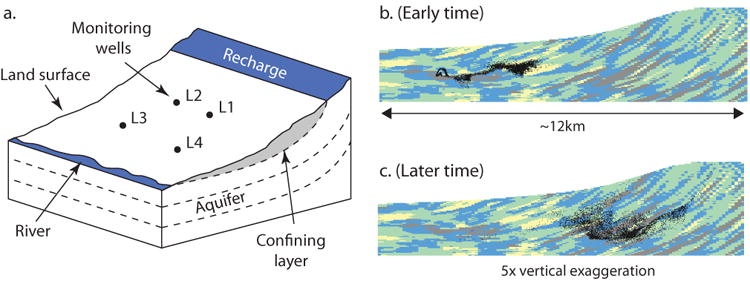
(a) Conceptual model of the regional scale aquifer, (b) Location of particles (black dots) at early time during the backwards in time simulation, and (c) Later time location illustrating the extent of dispersion within the aquifer. The colored regions in (b) and (c) represent discrete hydrofacies categories which increase in hydraulic conductivity from darker to lighter colors. (color version online)

Figure 3.

(a) Simulated age distributions from the backward in time particle tracking simulations, and (b) Tails of the cumulative distribution functions (CDF) for age. The 1-CDF scaling highlights the tailing and the divergent non-Fickian characteristics. (color version online)

Figure 4.

Advection-dispersion (ADE), fractional differential equation (FDE) resulting from the power law model, and truncated power law (TPL) model fits to the simulated age distributions (Sim) L2 and L4 (Figure 3). The FDE and TPL models both provide improvements over the previously derived Fickian (ADE) model. (color version online)

These simulations illustrate how consideration of heterogeneity of subsurface materials gives rise to non-Fickian age distributions on large scales as shown by Weissmann et al. [2002], and that a Fickian model is insufficient for describing such distributions. The TPL model seems to provide the best fit because of its ability to account for the different length scales of heterogeneity which is the cause of the non-Fickian behavior in this particular model. Matrix diffusion or mass transfer into immobile (zero velocity) regions may also produce non-Fickian age distributions [Varni and Carrera, 1998; Ginn et al., 2009] and the models shown here can also be applied to those processes.

5. Discussion and summary

The purpose of this article is to establish that the general model for age can be formulated from a random walk that is not restricted to Fickian conditions. Since most of this article focused on the goal of developing asymptotic, fractional differential equations that include age as a connection to previous works, we did not make use of the relationships developed in section 3.2 where the time and age PDFs were shown to be equivalent, though equation (3.10) conveys a fundamental result. Recall that the mass density distributed over time and age at all times, including pre-asymptotic times, is governed by the general solution of (3.13) or an alternate form where the space and time-age JPDFs are not decoupled. Particularly important is the condition required by equation (3.10) where the Dirac-delta of the conditional probability forced the marginal PDFs in time and age to be identical. In other words, they are always interchangeable. To illustrate the power of this equivalence, assume that the mass density at a particular location can be considered steady with respect to time. For a Dirac-delta in age, the distribution of mass density over the age dimension is the marginal PDF in age and, since the problem is steady in time, we can describe the age PDF with the existing CTRW tools, replacing time for age. From equation (3.10), we know that the time PDF will be identical to the known marginal PDF in age and we can then model the Green's function for the transport problem (with or without an age dimension). This implies that, given an age distribution, it may be possible to build an accurate, effective model of transport without requiring a tracer test or a groundwater model with highly resolved heterogeneity. The potential applications of these tools are quite promising since it can address one of the fundamental criticisms of non-Fickian transport modeling, which is that the parameters of the models cannot be determined a priori [Berkowitz et al., 2006; Neuman and Tartakovsky, 2009].

The physical processes that cause non-Fickian age distributions are the same processes that cause non-Fickian transport; the (steady-state case) age distribution for a water sample is also the solution of the solute transport (with age as time) for an instantaneous unit solute source at all recharge boundaries [Ginn et al., 2009]. Heterogeneities, mass transfer, sorption, and slow-advection are just some of the potential causes of non-Fickian age distributions but it is important to recognize that none of these processes will cause dispersion in the age dimension and neither will transience. In section 4.2, the non-Fickian age distributions in our example result from hydrodynamic dispersion caused by a wide range of velocities. This affects the amount of time it takes a given water molecule to travel from the source to a monitoring location but the aging velocity will always be unity as long as the water is in the aquifer. Similarly, a transient velocity field will affect the time a molecule of water spends in an aquifer by changing the path of the molecules but the aging rate will not change. This highlights one fundamental property of groundwater age that makes it an attractive tracer and model calibration tool because dispersion in the age distributions (Fickian or non-Fickian) can only be caused by the physical processes within the aquifer. If an age distribution in a natural aquifer is found to be non-Fickian, exploring the different non-Fickian models that can be applied to that distribution can reveal a great deal about the internal structure of that aquifer and the physical processes affecting solute transport and groundwater flow. So in addition to being a good candidate for an ideal tracer, groundwater age distributions are valuable tools for subsurface characterization.

In summary, we derived non-Fickian models of groundwater age distributions using a tagged-particle framework based on random walks. The general solution of the age equation was easily expressed in terms of arbitrary jump length PDFs in Fourier-Laplace space and the solutions can create Fickian or non-Fickian dispersion depending on the form of the PDFs selected. Connecting to previous work on fractional dynamics, we used the transition densities of Metzler and Klafter [2000] to highlight the differences between the transport and age equations for the case of time-age fractional dispersion. When the first two moments of the transition probability densities remain finite at late time/age and long distances, our general solution recovers an ensemble averaged, or effective, model of Fickian dispersion that is identical to the equation of Ginn et al. [2009] with constant coefficients. A notable distinction of the present derivation is that age was included as an additional dimension with time whereas Ginn [1999] included age as an analogy to a spatial dimension of the problem space. This required that all Laplace transforms of the continuous random walk be executed with respect to time and age and we showed that that the marginal PDFs in time and age must be identical via a coupled, conditional probability. Identical PDFs must have the same moments, so our coupled time-age JPDF provides a Lagrangian explanation for the equivalence of time and age moments [Harvey and Goerlick, 1995; Varni and Carrera, 1998; Ginn et al., 2009]. The equivalence also implies that knowledge of one marginal PDF gives complete knowledge of the other and that it may be possible to use an age distribution that is steady with respect to time to determine a the correct PDF for a given non-Fickian transport model without conducting a tracer test. We then showed several age distributions that were generated from numerical simulations within a geologically based synthetic example domain. The simulated distributions exhibited diverging characteristics that could not be described with a Fickian model and were fit more accurately using the proposed non-Fickian models of age.

Appendix A: Asymptotic approximation of the joint densities

The transition densities used to generate the governing differential equations and the general solutions are characterized by the asymptotic behavior of the functions. We derive the asymptotic behavior of the Laplace transformed joint PDF in time and age and the Fourier transformed PDF in space. The result of the following derivation is similar to Shlesinger [1974] but with Laplace transforms in time and age and is also similar to the approach outlined by Cushman and Ginn [1993]. Some authors have used special mathematical theorems to investigate the asymptotic behavior of the transition rates which is particularly useful when the moments do not exist [e.g. Montroll and Weiss, 1965; Scher and Montroll, 1975] but we outline a simple approach that works whenever the first two moments of the transition density functions exist.

The two dimensional Laplace transform can be written as

$$\stackrel{\sim }{\overline{f}}(s_t,s_a)=\underset{0}{\overset{\infty }{\int }}exp(-s_{a}a)\underset{0}{\overset{\infty }{\int }}exp(-s_{t}t)f(t,a)\mathrm{d}t\mathrm{d}a$$ (A.1)

The asymptotic behavior of f(t, a) will be dominated by the low frequency portion of the function which is the limiting behavior of the function as it goes to zero in Laplace space. Instead of their continuous functional form, the exponential functions in (A.1) can be approximated using a power series expansion about zero which is

$$exp(x)=\sum _{n=0}^{\infty }\frac{{(x)}^n}{n!}=1+x+\dots \vartheta$$ (A.2)

for the arbitrary function argument x, where ϑ represents higher order terms. Since the concern is the low frequency limit of the transition density, Shlesinger [1974] omitted the high order terms and retained only the first two terms of the expansion. We verified the validity of this assumption numerically by comparing the integral of the squared errors of the series expansion relative to the continuous exponential function near the origin and found that it is a reasonable approximation. Apply the low order series expansion approximation for the kernels of both Laplace transforms then combine (A.1) and the remaining terms of (A.2)

$$\stackrel{\sim }{\overline{f}}(s_t,s_a)=\underset{0}{\overset{\infty }{\int }}(1-s_{a}a)\underset{0}{\overset{\infty }{\int }}(1-s_{t}t)f(t,a)\mathrm{d}t\mathrm{d}a$$ (A.3)

Distributing the factors and carefully distributing the integration gives

$$\stackrel{\sim }{\overline{f}}(s_t,s_a)=\underset{0}{\overset{\infty }{\int }}(1-s_{a}a)[\underset{0}{\overset{\infty }{\int }}f(t,a)\mathrm{d}t-s_t\underset{0}{\overset{\infty }{\int }}tf(t,a)\mathrm{d}t]\mathrm{d}a$$ (A.4a)

$$\stackrel{\sim }{\overline{f}}(s_t,s_a)=\underset{0}{\overset{\infty }{\int }}\underset{0}{\overset{\infty }{\int }}f(t,a)\mathrm{d}t\mathrm{d}a-s_t\underset{0}{\overset{\infty }{\int }}\underset{0}{\overset{\infty }{\int }}tf(t,a)\mathrm{d}t\mathrm{d}a-s_a\underset{0}{\overset{\infty }{\int }}a\underset{0}{\overset{\infty }{\int }}f(t,a)\mathrm{d}t\mathrm{d}a+s_a{s}_t\underset{0}{\overset{\infty }{\int }}a\underset{0}{\overset{\infty }{\int }}tf(t,a)\mathrm{d}t\mathrm{d}a$$ (A.4b)

The first term is unity since it is the integral over the entire JPDF and the final term will be omitted since it can be deemed a higher order term because of the cross-multiplication of the Laplace parameters. Reversing the order of integration in the second term of (A.4b) and simplifying puts both inner integrals into the form of a marginal distribution

$$\stackrel{\sim }{\overline{f}}(s_t,s_a)=1-s_t\underset{0}{\overset{\infty }{\int }}t{f}_{\mathrm{T}}(t)\mathrm{d}t-s_a\underset{0}{\overset{\infty }{\int }}a{f}_{\mathrm{A}}(a)\mathrm{d}a$$ (A.5)

where f_T and f_A are the marginal PDFs in time and age, respectively. The remaining integrals are easily recognized as the first moments (or expectation) of the marginal PDFs in time and age; the first moment is sometimes called the characteristic scale or length of a particular dimension though the formal units are time in this case. An important point is that (A.5) is determined only by the marginal PDFs regardless of the form of the JPDF. For the groundwater age problem, the marginal PDFs in time and age must be identical and will have the same mean which was denoted as τ in this article. Comparing (3.14) to the finite moment case of Shlesinger [1974], the results are identical except for the extra term corresponding to the age dimension which is of identical form to the time term. The characteristic scales of a generalized exposure time need not be identical and it is a straightforward, conceptual, step to recognize that ratio of the characteristic exposure time and the first moment of the time PDF is the mean velocity in the exposure time (or age) dimension.

Using a similar technique, we can also approximate the low wave number behavior of a Fourier transformed transition density function. The Fourier-Transform can be defined as

$$\widehat{f}(k)=\underset{-\infty }{\overset{\infty }{\int }}exp(-ikx)f(x)\mathrm{d}x$$ (A.6)

Approximating the kernel with its series expansion to second order and inserting it into (A.6) gives

$$\widehat{f}(k)=\underset{-\infty }{\overset{\infty }{\int }}[1-ikx+\frac{1}{2}{(-ikx)}^2]f(x)\mathrm{d}x$$ (A.7)

Careful distribution of the exponent and integrals gives

$$\widehat{f}(k)=\underset{-\infty }{\overset{\infty }{\int }}f(\mathbf{x})\mathrm{d}x-ik\underset{-\infty }{\overset{\infty }{\int }}xf(x)\mathrm{d}x-\frac{1}{2}{k}^2\underset{-\infty }{\overset{\infty }{\int }}{x}^{2}f(x)\mathrm{d}x$$ (A.8)

Defining a mean displacement and variance term, one arrives at the simplified form

$$\widehat{f}(k)=1-ik\langle x\rangle -{\sigma }^2{k}^2$$ (A.9)

As with the previous models, the variance term is strictly the second raw moment. For distributions that are symmetric about the origin, the first moment will be zero and the second raw moment is also the variance because of the zero mean. When σ² represents the raw second moment about a non-zero mean, it is straight forward to convert the dispersion coefficient into one that is corrected by the square of the first moment, recovering a description of the variance.

The obvious limitation of this analysis is that it fails when the moments of the PDFs do not exist. For distributions with infinite mean, there are several approaches. If the transition density function can be defined in the time (or age) domain, the limit of the distribution as time goes to infinity can be approximated and Laplace transformed. The LT function can then be expanded as a power series about the origin to approximate the low frequency, asymptotic, form. Alternately, Tauberian theorems can be used which was the preferred method in the early continuous random walk work [e.g. Montroll and Weiss, 1965]. However, if the entire transition density is being considered, no asymptotic behavior approximation is needed and the resulting model will describe asymptotic and pre-asymptotic conditions but such models are not likely to invert from Fourier-Laplace space easily.

Appendix B: Fractional differintegration

Fractional differintegrals are generalizations of integer order integration and differentiaon to arbitrary integer orders. Benson et al. [2000] provide a good explanation of fractional derivatives which are “integer derivatives of partial integrals.” The Reimann-Liouville definition of the fractional derivative which is outlined in the text by Oldham and Spanier [1974] and is given as

$$\frac{{\mathrm{d}}^{-\alpha }}{\mathrm{d}{x}^{-\alpha }}f(x)=\frac{1}{\mathrm{\Gamma }(\alpha )}\underset{0}{\overset{x}{\int }}{(x-k)}^{\alpha -1}(k)\mathrm{d}xk$$ (B.1)

where Γ is the Gamma function and the lower limit of differintegration has been fixed at zero. Equation (B.1) is a convolution and it is through the specific form of the convolution kernel that fractional-derivative based models have been be related to more general nonlocal models of transport [e.g. Cushman and Ginn, 2000]. The notation to describe fractional operators given by Oldham and Spainer is quite convenient: a differintegral can be written as d^q/dt^q where q is the real number order of differintegration that results in a derivative for q > 0 and an integral for q < 0 but note that this notation implies that the lower limit of differintegration is zero. In the manuscript we make use of the Laplace transform to generate real space fractional order differential equations. The Laplace transform of a differintegral can be generalized to arbitrary order as

$$\ell \left\{\frac{{\mathrm{d}}^{q}f(t)}{\mathrm{d}{t}^q}\right\}=s^q\ell \{f\}-\sum _{k=0}^{n-1}{s}^k\frac{{\mathrm{d}}^{q-1-k}}{\mathrm{d}{t}^{q-1-k}}f(0)$$ (B.2)

where ℓ{*} denotes the LT operation, n is the first integer larger than q, k is an integer order index, and s is the Laplace parameter [Oldham and Spanier, 1974]. When q < 0 the differintegral being Laplace transformed is an integral and the terms of the summation are null; this was the case in equation (4.9). The LT of the general differintegral of some constant, C, is also used in this manuscript:

$$\ell \left\{\frac{{\mathrm{d}}^{-q}C}{\mathrm{d}{t}^{-q}}\right\}=s^{-q}\ell \{C\}=s^{-q}\left(\frac{C}{s}\right)=s^{-1-q}C$$ (B.3a)

$$\frac{{\mathrm{d}}^{-q}C}{\mathrm{d}{t}^{-q}}={\ell }^{-1}\left\{s^{-(1+q)}C\right\}$$ (B.3b)

where ℓ⁻¹{*} denotes the inverse LT with 0 < q ≤ 1 [Oldham and Spanier, 1974]. Unlike integer order differentiation, fractional differentiation of a constant does not result in a zero which is most apparent in the current article when comparing the Fickian and non-Fickian differential equations. Using these definitions, it is straight forward to modify the general result of section 4.1 to a time-age fractional derivative in the interval 1 < q ≤ 2; this has been noted by several authors for a time-fractional CTRW model [e.g. Berkowitz et al., 2002; Zhang et al., 2009].

References

- Barkai E, Fleurov VN. Levy walks and generalized stochastic collision models. Physical Review E. 1997;56(6):6355–6361. [Google Scholar]
- Benson DA, Wheatcraft SW, Meerschaert MM. The fractional-order governing equation of Levy motion. Water Resources Research. 2000;36(6):1413–1423. [Google Scholar]
- Berkowitz B, Scher H. Theory of anomalous chemical transport in random fracture networks. Physical Review E. 1998;57(5):5858–5869. [Google Scholar]
- Berkowitz B, Scher H. The role of probabilistic approaches to transport theory in heterogeneous media. Transport in Porous Media. 2001;42(1-2):241–263. [Google Scholar]
- Berkowitz B, Emmanuel S, Scher H. Non-Fickian transport and multiple-rate mass transfer in porous media. Water Resources Research. 2008;44(3) [Google Scholar]
- Berkowitz B, Klafter J, Metzler R, Scher H. Physical pictures of transport in heterogeneous media: Advection-dispersion, random-walk, and fractional derivative formulations. Water Resources Research. 2002;38(10) [Google Scholar]
- Berkowitz B, Cortis M, Dentz M, Scher H. Modeling non-Fickian transport in geological formations as a continuous time random walk. Reviews of Geophysics. 2006;44(2) [Google Scholar]
- Bhattacharya R, Gupta VK. Application of central limit theorems to solute dispersion in saturated porous media: From kinetic to field scales. In: Cushman JH, editor. Dynamics of Fluids in Hierarchical Porous Media. Academic Press; San Diego, CA: 1990. p. 505. [Google Scholar]
- Bohlke J, Denver J. Combined use of groundwater dating, chemical, and isotopic analyses to resolve the history and fate of nitrate contamination in 2 agricultural watersheds, Atlantic coastal-plain, Maryland. Water Resources Research. 1995;31(9):2319–2339. [Google Scholar]
- Carle SF, Fogg GE. Transition probability-based indicator geostatistics. Mathematical Geology. 1996;28(4):453–476. [Google Scholar]
- Carrera J, Sanchez-Vila X, Benet I, Medina A, Galarza G, Guimera J. On matrix diffusion: formulations, solution methods and qualitative effects. Hydrogeology Journal. 1998;6(1):178–190. [Google Scholar]
- Cook PG, Love AJ, Robinson NI, Simmons CT. Groundwater ages in fractured rock aquifers. Journal of Hydrology. 2005;308(1-4):284–301. [Google Scholar]
- Corcho Alvarado JA, Purtschert R, Barbecot F, Chabault C, Rueedi J, Schneider V, Aeschbach-Hertig W, Kipfer R, Loosli HH. Constraining the age distribution of highly mixed groundwater using 39 Ar: A multiple environmental tracer (H-3/He-3, Kr-85, Ar-39, and C-14) study in the semiconfined Fontainebleau Sands Aquifer (France) Water Resources Research. 2007;43(3) [Google Scholar]
- Cornaton FJ. Transient water age distributions in environmental flow systems: The time-marching Laplace Transform solution technique. Water Resources Research. 2012 doi: 10.1029/2011WR010606. in press. [DOI] [Google Scholar]
- Cornaton F, Perrochet P. Groundwater age, life expectancy and transit time distributions in advective-dispersive systems: 1. Generalized reservoir theory. Advances in Water Resources. 2006;29(9):1267–1291. [Google Scholar]
- Cortis A, Berkowitz B. Computing “Anomalous” contaminant transport in porous media: The CTRW MATLAB toolbox. Ground Water. 2005;43(6):947–950. doi: 10.1111/j.1745-6584.2005.00045.x. [DOI] [PubMed] [Google Scholar]
- Cortis A, Gallo C, Scher H, Berkowitz B. Numerical simulation of non-Fickian transport in geological formations with multiple-scale heterogeneities. Water Resources Research. 2004;40(4) [Google Scholar]
- Cushman JH, Ginn TR. Nonlocal dispersion in media with continuously evolving scales of heterogeneity. Transport in Porous Media. 1993;13(1):123–138. [Google Scholar]
- Cushman JH, Ginn TR. Fractional advection-dispersion equation: A classical mass balance with convolution-Fickian flux. Water Resources Research. 2000;36(12):3763–3766. [Google Scholar]
- Cvetkovic V, Dagan G, Cheng H. Contaminant transport in aquifers with spatially variable hydraulic and sorption properties. Proceedings of the Royal Society of London Series a-Mathematical Physical and Engineering Sciences. 1998;454(1976):2173–2207. [Google Scholar]
- Dentz M, Berkowitz B. Transport behavior of a passive solute in continuous time random walks and multirate mass transfer. Water Resources Research. 2003;39(5) [Google Scholar]
- Dentz M, Cortis A, Scher H, Berkowitz B. Time behavior of solute transport in heterogeneous media: transition from anomalous to normal transport. Advances in Water Resources. 2004;27(2):155–173. [Google Scholar]
- Engdahl NB, Weissmann GS. Anisotropic transport rates in heterogeneous porous media. Water Resources Research. 2010;46 [Google Scholar]
- Fogg GE, Noyes CD, Carle SF. Geologically based model of heterogeneous hydraulic conductivity in an alluvial setting. Hydrogeology Journal. 1998;6(1):131–143. [Google Scholar]
- Fogg GE, LaBolle EM, Weissmann GS. Groundwater vulnerability assessment: Hydrogeologic perspective and example from Salinas Valley, California. In: Corwin DL, Loague K, Ellsworth TR, editors. Application of GIS, Remote Sensing, Geostatistical and Solute Transport Modeling. AGU Geophysical Monograph; 1999. [Google Scholar]
- Ginn TR. On the distribution of multicomponent mixtures over generalized exposure time in subsurface flow and reactive transport: Foundations, and formulations for groundwater age, chemical heterogeneity, and biodegradation. Water Resources Research. 1999;35(5):1395–1407. [Google Scholar]
- Ginn TR, Haeri H, Massoudieh A, Foglia L. Notes on Groundwater Age in Forward and Inverse Modeling. Transport in Porous Media. 2009;79(1):117–134. [Google Scholar]
- Goode DJ. Direct simulation of groundwater age. Water Resources Research. 1996;32(2):289–296. [Google Scholar]
- Harvey CF, Gorelick SM. Temporal moment-generating equations: Modeling and mass transfer in heterogeneous aquifers. Water Resources Research. 1995;31(8):1895–1911. [Google Scholar]
- Klafter J, Silbey R. Derivation of the continuous-time random-walk equation. Physical Review Letters. 1980;44(2):55–58. [Google Scholar]
- Klafter J, Blumen A, Shlesinger MF. Stochastic pathway to anomalous diffusion. Physical Review A. 1987;35(7):3081–3085. doi: 10.1103/physreva.35.3081. [DOI] [PubMed] [Google Scholar]
- LaBolle EM. RWHet: Random walk particle model for simulating transport in heterogeneous permeable media, user's manual and program documentation, Version 4.1. University of California; Davis: 2010. p. 27. [Google Scholar]
- LaBolle E, Fogg G, Tompson A. Random-walk simulation of transport in heterogeneous porous media: Local mass-conservation problem and implementation methods. Water Resources Research. 1996;32(3):583–593. [Google Scholar]
- LaBolle EM, Fogg GE. Role of molecular diffusion in contaminant migration and recovery in an alluvial aquifer system. Transport in Porous Media. 2001;42(1-2):155–179. [Google Scholar]
- LaBolle EM, Fogg GE, Eweis JB. Diffusive fractionation of H-3 and He-3 in groundwater and its impact on groundwater age estimates. Water Resources Research. 2006;42(7) [Google Scholar]
- Larocque M, Cook PG, Haaken K, Simmons CT. Estimating Flow Using Tracers and Hydraulics in Synthetic Heterogeneous Aquifers. Ground Water. 2009;47(6):786–796. doi: 10.1111/j.1745-6584.2009.00595.x. [DOI] [PubMed] [Google Scholar]
- Lassey KR. Unidimensional solute transport incorporating equilibrium aand rate-limited isotherms with 1st-order loss: 1. Model conceptualizations and analytic solutions. Water Resources Research. 1988;24(3):343–350. [Google Scholar]
- Lee SY, Carle SF, Fogg GE. Geologic heterogeneity and a comparison of two geostatistical models: Sequential Gaussian and transition probability-based geostatistical simulation. Advances in Water Resources. 2007;30(9):1914–1932. [Google Scholar]
- Maloszewski P, Zuber A. Determining the turnover time of groundwater systems with the aid of environmental tracers. 1. Models and their applicability. Journal of Hydrology. 1982;57(3-4):207–231. [Google Scholar]
- Massoudieh A, Ginn TR. The theoretical relation between unstable solutes and groundwater age. Water Resources Research. 2011;47 [Google Scholar]
- Metzler R, Klafter J. The random walk's guide to anomalous diffusion: a fractional dynamics approach. Physics Reports-Review Section of Physics Letters. 2000;339(1):1–77. [Google Scholar]
- Metzler R, Klafter J, Sokolov IM. Anomalous transport in external fields: Continuous time random walks and fractional diffusion equations extended. Physical Review E. 1998;58(2):1621–1633. [Google Scholar]
- Montroll EW, Weiss GH. Random walks on lattices 2. Journal of Mathematical Physics. 1965;6(2):167–181. [Google Scholar]
- Neuman SP, Tartakovsky DM. Perspective on theories of non-Fickian transport in heterogeneous media. Advances in Water Resources. 2009;32(5):670–680. [Google Scholar]
- Neumann RB, Labolle EM, Harvey CF. The effects of dual-domain mass transfer on the tritium-helium-3 dating method. Environmental Science & Technology. 2008;42(13):4837–4843. doi: 10.1021/es7025246. [DOI] [PubMed] [Google Scholar]
- Oldham KB, Spanier J. The Fractional Calculus: Theory and Applications of Differentiation and Integration to Arbitrary Order. Dover Publications Inc.; Mineola, NY: 1974. [Google Scholar]
- Sanford W. Calibration of models using groundwater age. Hydrogeology Journal. 2011;19(1):13–16. [Google Scholar]
- Scher H, Lax M. Stochastic transport in a disordered solid: 1. Theory. Physical Review B. 1973;7(10):4491–4502. [Google Scholar]
- Scher H, Montroll EW. Anomalous transit-time dispersion in amorphous solids. Physical Review B. 1975;12(6):2455–2477. [Google Scholar]
- Seeboonruang U, Ginn TR. Upscaling heterogeneity in aquifer reactivity via exposure-time concept: Forward model. Journal of Contaminant Hydrology. 2006;84(3-4):127–154. doi: 10.1016/j.jconhyd.2005.12.011. [DOI] [PubMed] [Google Scholar]
- Shlesinger MF. Asymptotic solutions of continuous-time random-walks. Journal of Statistical Physics. 1974;10(5):421–434. [Google Scholar]
- Varni M, Carrera J. Simulation of groundwater age distributions. Water Resources Research. 1998;34(12):3271–3281. [Google Scholar]
- Weissmann GS, Zhang Y, LaBolle EM, Fogg GE. Dispersion of groundwater age in an alluvial aquifer system. Water Resources Research. 2002;38(10) [Google Scholar]
- Willmann M, Carrera J, Sanchez-Vila X. Transport upscaling in heterogeneous aquifers: What physical parameters control memory functions? Water Resources Research. 2008;44(12) [Google Scholar]
- Woolfenden LR, Ginn TR. Modeled Ground Water Age Distributions. Ground Water. 2009;47(4):547–557. doi: 10.1111/j.1745-6584.2008.00550.x. [DOI] [PubMed] [Google Scholar]
- Zhang Y, Benson DA, Reeves DM. Time and space nonlocalities underlying fractional-derivative models: Distinction and literature review of field applications. Advances in Water Resources. 2009;32(4):561–581. [Google Scholar]
- Zinn BA, Konikow LF. Potential effects of regional pumpage on groundwater age distribution. Water Resources Research. 2007;43(6) [Google Scholar]