Laboratory and Field Study of the Potential Benefits of Pinna Cue-Preserving Hearing Aids

Abstract

The potential benefits of preserving high-frequency spectral cues created by the pinna in hearing-aid fittings were investigated in a combined laboratory and field test. In a single-blind crossover design, two settings of an experimental hearing aid were compared. One setting was characterized by a pinna cue-preserving microphone position, whereas the other was characterized by a microphone position not preserving pinna cues. Participants were allowed 1 month of acclimatization to each setting before measurements of localization and spatial release from speech-on-speech masking were completed in the laboratory. Real-world experience with the two settings was assessed by means of questionnaires. Seventeen participants with mild to moderate sensorineural hearing impairments completed the study. An inconsistent pinna cue benefit pattern was observed across the outcome measures. In the localization test, the pinna cue-preserving setting provided a significant mean reduction of 22° in the root mean square (RMS) error in the front–back dimension, with 13 of the 17 participants showing a reduction of at least 15°. No significant mean difference in RMS error between settings was observed in the left–right dimension. No significant differences between settings were observed in the spatial-unmasking test conditions. The questionnaire data indicated a small, but nonsignificant, benefit of the pinna cue-preserving setting in certain real-life situations, which corresponded with a general preference for that setting. No significant real-life localization benefit was observed. The results suggest that preserving pinna cues can offer benefit in some conditions for individual hearing-aid users with mild to moderate hearing loss and is unlikely to harm performances for the rest.

Introduction

Spatial hearing is an important ability. It enables listeners to localize sound sources, and furthermore, it can improve listeners’ ability to understand speech in the presence of competing sound sources. This is the case when the competing sound sources are spatially separated, allowing a number of acoustical and perceptual mechanisms to come into play such that a spatial release from masking (SRM) can occur (e.g., Bronkhorst, 2000; Freyman, Helfer, McCall, & Clifton, 1999; Zurek, 1993).

A listener’s ability to locate the spatial origin of a sound stems from three fundamental types of acoustical cues: interaural time differences (ITDs), interaural level differences (ILDs), and monaural spectral cues (see Blauert, 1997, for a review). The binaural cues (ITDs and ILDs) provide information about a sound source’s position in the horizontal plane (the left–right [L–R] dimension), whereas they provide no information about the position in the median vertical plane (the front–back [F–B] and up–down dimensions). The ability to localize sound sources in the latter plane requires access to monaural spectral cues. These cues arise from the filtering of the incident sound, which is introduced by the human torso, the head, and, in particular, the outer ear. This filtering depends on the angle of incidence and results in characteristic spectral changes above approximately 2 kHz (Mehrgardt & Mellert, 1977).

For listeners with a sensorineural hearing loss, localization performance is degraded compared with normal-hearing listeners (e.g., Häusler, Colburn, & Marr, 1983; Lorenzi, Gatehouse, & Lever, 1999; Noble Byrne, & LePage, 1994; Rakerd, Vander Velde, & Hartmann, 1998). The use of independently operating bilateral hearing aids further deteriorates localization performance compared with unaided performance when sufficient audibility of the stimuli in the unaided condition is provided (e.g., Orton & Preves, 1979; Van den Bogaert, Carette, & Wouters, 2011; Van den Bogaert, Klasen, Moonen, Van Deun, & Wouters, 2006). The decrease in localization performance introduced by independently operating bilateral hearing aids is thought to be partly due to disruption of the binaural ITD and ILD cues caused by, for example, nonsynchronized behavior of adaptive signal processing strategies across ears (Keidser et al., 2006), and partly due to disruption of the monaural spectral cues provided by pinna filtering (Van den Bogaert, Carette, & Wouters, 2009). The disruption of these pinna cues is known to cause increases in elevation errors and F–B confusion (e.g., Asano, Suzuki, & Sone, 1990; Butler, 1986; Musicant & Butler, 1984). The disruption of pinna cues introduced by the hearing aid can, for example, be due to a limited bandwidth of the hearing aid, which restricts the listener from getting access to some of the high-frequency pinna cues (e.g., Butler, 1986). In recent years, this problem has been addressed by increasing the frequency-response bandwidth in hearing aids.

Another very basic cause of disruption of pinna cues is the position of the hearing-aid (HA) microphone. For example, on behind-the-ear (BTE) styles, the microphone position is behind, or at, the top of the outer ear, meaning that sounds are picked up and processed before they have been filtered by the natural pinna cues. This is in contrast to in-the-ear (ITE) styles of hearing aids, which have the microphone positioned at the entrance to (or inside) the ear canal, meaning that access to the natural pinna cues is maintained (Hammershøi & Møller, 1996). BTE devices have recently gained increasing popularity due to the possibility of offering open-ear acoustics (e.g., Flynn, 2003). Although this provides relief to occlusion, it is possible that users are disadvantaged in terms of being denied access to the pinna cues that are important for spatial hearing. A number of studies have compared ITE and BTE hearing aids and have shown better localization performance (in the F–B dimension) with ITE hearing aids in hearing-impaired (HI) listeners (Orton & Preves, 1979; Türk, 1986; Westermann & Tøpholm, 1985) or no difference in localization performance (Byrne, Noble, & Lepage, 1992; Leeuw & Dreschler, 1987). The lack of difference between ITE and BTE observed in the two latter studies might be explained by procedural issues, for example, allowing head movements during localization tests (facilitating benefit of binaural cues), using narrowband noise centered at frequencies where pinna cues are modest, or excluding presentations from behind the listener.

A more recent study by Best et al. (2010) compared localization with a completely-in-the-canal (CIC) hearing aid, which offers a deeper microphone position than the ITE style, with localization with a BTE hearing aid in a group of HI people. They found that the CIC offered a localization benefit over the BTE, in the form of fewer occurrences of F–B confusion, whereas no difference was observed for lateral or vertical localization errors. The lack of difference in the vertical dimension was explained by limited high-frequency gain in the CIC hearing aid used in the study. Furthermore, they found that 4 to 6 weeks of acclimatization improved localization with both types of hearing aids. Van den Bogaert et al. (2011) compared localization performance with different HA styles in a group of HI people, who wore the hearing aids in the laboratory only (thus, without any substantial acclimatization). No difference between HA styles in L–R localization performance was observed, whereas F–B localization performance with a BTE hearing aid equipped with an omnidirectional microphone was worse than with the other styles. The other styles included an open-fitting BTE with directional microphone, an in-the-canal (ITC) hearing aid, and an in-the-pinna (ITP) hearing aid with the microphone positioned in the pinna. Between these three styles, no differences in F–B localization performance were found.

The previously mentioned studies did not investigate whether the observed improvements in F–B localization provided by preservation of pinna cues were accompanied by improvements in speech intelligibility, in particular in the F–B dimension. The spectral cues could potentially be useful in unmasking of speech coming from the front when a masking signal is coming from the back. The question whether this is the case is only sparsely addressed in the literature. In a group of normal-hearing listeners, Rychtáriková, Van den Bogaert, Vermeir, & Wouters (2011) compared localization and speech-intelligibility performance with preservation of pinna cues to performance without preservation of pinna cues. In anechoic conditions, they found a benefit of preservation of pinna cues in F–B localization and in a speech intelligibility test with speech presented at 0° and stationary noise presented at 180°. Furthermore, they found a moderate correlation between the increase in the ability for F–B localization and the improvement of speech intelligibility when the signal and noise were separated by 180°. This indicates that preservation of pinna cues could improve localization and speech understanding in the F–B dimension. Even though the data indicate that the pinna cues were more important for the localization task than for the spatial-unmasking task, this finding supports the hypothesis that preservation of pinna cues could be beneficial for localization and for SRM in the F–B dimension. It should be noted that some of the test conditions in their study were realized through headphone listening by applying a head-related transfer function (HRTF) recorded either in the ear of an artificial head or at the microphone position of a BTE hearing aid positioned on an artificial head. The listeners were not acclimatized to the nonpersonalized spectral cues available in these test conditions.

The studies on the effects of different microphone locations referred to earlier were all based on data collected in the laboratory. Even though some of them included an acclimatization period before conducting tests in the laboratory, none of the studies attempted to investigate whether the effects of microphone location found in the laboratory were perceived by the participants in real life. From studies on other types of HA functionality, for example, directional microphones, it is known that benefits measured in laboratory tests may not be reflected by benefits perceived by users in their everyday life (e.g., Walden, Surr, Cord, Edwards, & Olson, 2000). However, when listening situations in everyday life match the ideal conditions in the laboratory, the correspondence between laboratory and real-life results is improved (Cord, Surr, Walden, & Olson, 2002).

The purpose of the present study was to further investigate the potential benefits offered to HI people by preserving pinna cues when fitted with hearing aids. In this context, preservation of pinna cues means that these cues, to the extent offered by the HA technology, are made available in the electrical signal processed by the hearing aid and made audible in the acoustic signal presented to the individual HA user. The purpose was accomplished by conducting a single-blind crossover field study where a group of participants with mild to moderate sensorineural hearing impairments compared two different HA microphone positions implemented in the same hearing aid: one preserving and one not preserving pinna cues. To optimize preservation of pinna cues, gain was prescribed to ensure sufficient audibility up to at least 8 kHz. Furthermore, a 1-month acclimatization period was included (for each setting) to enable adaptation to the available spatial cues. As in most previous investigations of perceived microphone location effects, a localization experiment was included in the present study, but to assess possible effects of pinna cue preservation on SRM, a test of spatial release from speech-on-speech masking (Neher et al., 2009) was included as well. Because the purpose was to investigate the effect of pinna cues, the focus was on performance in the F–B dimension in both the localization and SRM tests. The hypothesis was that the pinna cue-preserving setting would offer a benefit over the other setting in this dimension. However, performance in the L–R dimension, where the binaural spatial cues come into play, was assessed as well. In this dimension, the hypothesis was that no difference between settings would be observed. Besides testing in the laboratory, perceived differences between the two settings in everyday life were assessed by means of the Speech, Spatial, and Qualities of Hearing Scale-Comparative (SSQ-C) questionnaire (Jensen, Akeroyd, Noble, & Naylor, 2009).

Methods

Participants

An a priori power analysis was conducted to estimate the sample size needed to show a significant benefit of the pinna cue-preserving setting at a .05 significance level and with a statistical power of .8. The power analysis was based on performance in the SRM test. The effect size was the difference in speech reception threshold (SRT) between settings, analyzed with a one-sample two-tailed t test. With an effect size of 2.0 dB and a standard deviation of 2.0 dB (estimated from previous data), the power analysis resulted in a needed sample size of 10 listeners. Twenty HI participants were recruited for the study. During the course of the study, 3 participants dropped out either due to an inability to accept the sound of their own voice or due to technical problems with the hearing aids. Thus, 17 participants completed the study. Another power analysis showed that this sample size allowed for an effect size of 1.4 dB to be shown with the standard deviation and the levels of significance and power mentioned earlier.

In the following, only data from the 17 participants who completed the study are reported. The 17 participants included 6 females and 11 males, aged 42 to 73 years (mean = 62.5 years). They all had sensorineural, gently sloping hearing losses in the mild to moderate range. The four frequency average hearing loss (4FAHL), measured across 0.5, 1, 2, and 4 kHz and across both ears, was in the range of 27 to 51 dB HL (mean = 40 dB HL). Figure 1 shows the mean audiograms of the left and right ears. Some amount of residual high-frequency hearing was required to enable access to spectral cues within the entire bandwidth of the experimental hearing aid (see later). The participants had average high-frequency hearing losses, measured across 2, 4, 6, and 8 kHz and across both ears, of 44 to 64 dB HL (mean = 55 dB HL). They had symmetrical hearing losses, with the difference in 4FAHL across ears not exceeding 10 dB for any participant but allowing three participants to have differences across ears of 20 dB at single audiometric frequencies.

Figure 1.

Mean hearing threshold levels for right and left ears of the 17 participants.

Note. The error bars indicate ±1 standard deviation.

All participants were experienced HA users and had been fitted bilaterally with hearing aids for at least 1 year. The majority (15) of the participants used BTE devices (all being open fittings or having large vents with effective vent diameters between 3 and 9 mm); 1 participant used an ITC device (vent diameter 1.4 mm), and 1 participant used a CIC device (vent diameter 1.4 mm). The participants were selected based on their ability to take advantage of pinna cues in a preceding candidature study (Neher, Laugesen, Jensen, & Kragelund, 2011), as indicated by the level of unaided (open ear) performance in the same localization and SRM tests that were used in the present study, but with sound stimuli made audible to the individual listener by applying gain and spectral shaping based on the hearing loss. The participants were reimbursed for their travel expenses but otherwise not paid for their participation.

Experimental Hearing Aids

The hearing aid used in the field study was a modified version of the Oticon Epoq XW BTE 312 (Oticon, Smørum, Denmark), which offers a bandwidth of approximately 9 kHz. When compared with the commercially available version of the hearing aid, two major modifications were introduced. The first modification was that one of the hearing aid’s two omnidirectional microphones was removed from the BTE shell and placed in an acrylic earmold, which was custommade for each participant. When the hearing aid was in place, the microphone then had a position corresponding to the microphone position in a deeply fitted CIC hearing aid. The microphone was connected to the BTE shell via a thin wire placed next to the tube transmitting sound from the receiver in the BTE shell to the earmold. By implementing the two different microphone positions in the same physical hearing aid, the participants were blinded to the difference between the two settings. The experimental hearing aid is shown in Figure 2, in which the positions of the two microphones are indicated. All earmolds had a 1.4-mm collection vent.

Figure 2.

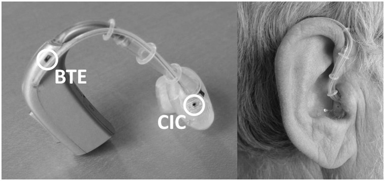
The experimental hearing aid used in the study with circles indicating the two microphone positions is shown (left). The hearing aid when positioned in the ear of one of the participants is shown (right). The opening of the 1.4-mm collection vent of the earmold is hidden behind the sound tube.

The switching between the two settings of the hearing aid, in the following just referred to as CIC (microphone positioned in the earmold) and BTE (conventional microphone position), was performed in the experimental fitting software, and appropriate acoustical transformations were applied to compensate for microphone location effects to equalize gain for frontal sound incidence in the two settings. The acoustical transformations regarding microphone location effects were based on internal measurements made at Oticon headquarters, in accordance with IEC 60118-8 (2005). The overall gains of the two settings were finally equalized by measurements in an anechoic test box (type 4232, Brüel & Kjær, Nærum, Denmark) with a 1-kHz sinusoid presented at 74 dB sound pressure level (SPL). In this way, the frequency response and the compression curve (input–output function) were the same for the two settings for sounds impinging from the front. For other directions of sound incidence, the difference in microphone position introduces spectral differences. Although these spectral differences directly represent the experimental contrast of interest, there is a potential undesired confounding side effect, which is a potential difference in disruptions to ITD and ILD cues between the two settings. However, according to Keidser et al. (2006), ITD cues are not disrupted in a hearing aid without a directional microphone (as used in the present study). Regarding ILD cues, Keidser et al. concluded that compression and noise reduction (which were present in the hearing aids used here) “shifted the magnitude of the ILDs, but had no further effect of clinical significance” (2006, p. 578). Hence, we would not expect any difference of consequence in the disruptions to ILD cues between the two settings tested here.

The spectral effect of each of the two microphone positions, relative to the front direction, is illustrated in Figure 3. The measurements shown in the figure were obtained for different angles of sound incidence from one set of the experimental hearing aids while worn by one of the participants. The participant was placed in the loudspeaker setup, which also was used for the perceptual tests (see later). The measurements were made at the output of the HA filter bank before the acoustical transformations mentioned earlier were applied. The figure shows that both microphone positions could provide a substantial spectral change of up to approximately 15 dB relative to the front direction. Differences of the same magnitude between the two microphone positions can also be observed in the figure. Similar measurements were not performed in the open ear, and the spectral effect of the CIC microphone position can thus not be compared directly with the spectral effect of the open ear. However, according to Hammershøi and Møller (1996), the spatial information in the signal can be assumed to be preserved at the CIC microphone position. Thus, the expected spectral difference between the CIC and the open-ear conditions only reflects the open-ear gain.

Figure 3.

Spectral changes, relative to 0°, at the CIC and BTE microphone positions for sounds coming from different azimuths (loudspeakers 4, 9, and 13 in Figure 5).

Note. The measurements were made at the filter-bank outputs of the experimental hearing aids of one of the participants who wore the hearing aids during the measurements. Measurements were made on the ipsilateral and the contralateral hearing aid. To ease readability of the plot, the 120° data have been offset by ±20 dB while the 45° data have been offset by ±40 dB. CIC = completely-in-the-canal; BTE = behind-the-ear.

The other major modification of the hearing aid concerned the gain prescription. The starting point was the voice aligned compression (VAC) active rationale (see Neher et al., 2009), which is the propriety procedure for fitting of the Epoq hearing aid (Oticon). This rationale was modified to ensure audibility of the high-frequency pinna cues that were the focus of this study, without compromising the provision of a generally well-performing and usable HA fitting. This was accomplished by defining an audibility target and, if necessary, increasing the insertion gain (originally prescribed by the VAC rationale) to amplify the audibility target to the hearing threshold. The audibility target was based on a reference long-term speech spectrum, averaged over male and female talkers, which was taken from Cox and Moore (1988) and adjusted to 65 dB SPL. However, when the long-term average spectrum of speech is computed, such as the Cox and Moore spectrum, the levels at high frequencies actually underestimate the levels of the important high-frequency speech components (short consonant sounds that occur relatively infrequently). Therefore, the reference spectrum was modified to take into account the temporal sparsity of high-frequency information in a running speech signal. The high-frequency modification was based on an analysis of one of the single-talker signals used in the SRM test (see later). The high-frequency speech components of the speech signal were identified, and the long-term spectrum of these was computed in isolation. At frequencies where this spectrum exceeded the overall long-term spectrum of the speech signal, a high-frequency sparsity adjustment was calculated as the difference between the two spectra. The adjustment was about 10 dB at frequencies above 4 kHz. A similar analysis of another single-talker signal provided almost identical results.

Figure 4 shows the reference speech spectrum (transformed to sound pressure level at the eardrum by adding a diffuse field to eardrum correction; Moore, Stone, Fullgrabe, Glasberg, & Puria, 2008) and the audibility target, which was obtained by adding the abovementioned high-frequency sparsity adjustment to the reference speech spectrum. At each audiometric frequency, the audibility target was quantized in 5-dB steps in accordance with the resolution of the aided-threshold measurements, which were performed to verify that the target was made audible (see later).

Figure 4.

The reference speech signal (Cox & Moore, 1988) corresponding to an overall level of 65 dB SPL, the audibility target obtained by adding the high-frequency sparsity adjustment and quantizing to 5-dB steps, and the mean aided thresholds (±1 standard deviation) across participants and ears (after gain adjustments were made).

Note. All sound pressure levels correspond to a position at the eardrum and to one-third octave bands centered at the indicated audiometric frequencies.

The initial fitting of the hearing aid was always performed in the CIC setting where the occurrence of acoustic feedback was considered most likely due to the increased feedback loop response magnitude of the CIC microphone position relative to the BTE microphone position. To verify that the defined audibility targets were being met (i.e., that the target was audible at all frequencies), aided-threshold measurements were performed in an audiometric booth with one-third octave-band noise stimuli at audiometric frequencies up to and including 8 kHz. The aided thresholds were measured separately for each ear, with the other ear blocked by an ear muff. In those cases where a target was not met at one or more frequencies, the hearing aid’s gain for low-level inputs was increased according to the difference between threshold and target. The gain for high-level inputs remained unchanged, and the effective compression ratio was thus increased. The gain adjustment at low input levels was made to obtain the desired level of audibility while avoiding excessive gain at high input levels, which potentially could make the hearing aids intolerable during real-life use. Deviations that required an increase of gain were few for frequencies below 8 kHz, but at 8 kHz, adjustments were typically required. The mean deviation from the audibility target (i.e., the required increase of gain) at 8 kHz, across participants and ears, was approximately 5 dB, with the maximum individual deviation being 15 dB. The final mean-aided thresholds, after gain adjustments were made, are also shown in Figure 4. The fact that gain typically had to be increased at 8 kHz meant that the aided threshold at that frequency was just at target for most of the participants. All targets were met except for two cases, where the 8-kHz target could not be met because of acoustic feedback.

Due to an error in the experimental fitting software, which was first discovered toward the end of the study, approximately 4 dB of additional gain (compared with the prescribed gain) was applied in the BTE setting for frequencies above approximately 5 kHz (the gain error occurred after the filter bank and thus does not affect the measurements shown in Figure 3). Nevertheless, because aided-threshold measurements were completed for the CIC setting to ensure that audibility requirements were met, the gain error did not compromise the intended audibility and the preservation of pinna cues in either setting.

Directional microphones were not activated in the experimental hearing aids. The noise reduction and antifeedback features were enabled during the field test, while the volume control was disabled. Those participants who had an Oticon, Smørum, Denmark as part of their own HA system (enabling wireless communication between the hearing aids and, e.g., a mobile phone) were also able to use it with the experimental hearing aid during the field test.

Spatial Listening Tasks

Sound localization

All sound localization measurements were carried out under anechoic conditions. Thirteen active Genelec 8030A loudspeakers (Genelec, Iisalmi, Finland) were positioned in the horizontal plane in a semicircular arrangement with an angular separation of 15° (see Figure 5). The distance between the loudspeakers and the listening position was 1.5 m. The loudspeakers were connected directly to a 24-channel sound card (MOTU Audio 24I/O, MOTU, Cambridge, MA), which in turn was connected to a computer running the experimental software written in MATLAB.

Figure 5.

Loudspeaker setup used for the localization and SRM tests.

Note. The localization test setup includes the loudspeakers numbered 1 to 13 on one side of the participant (the figure illustrates a right-side test; a left-side test is performed in a mirrored setup). The loudspeakers included in the SRM test setup are marked with gray. In the SRM test, the target speech signal (T) is always presented from the frontal loudspeaker, whereas the loudspeakers presenting the two masker speech signals (M) depend on the masking condition (colocated, displaced F–B, or displaced L–R, as indicated in the figure). SRM = spatial release from masking; F–B = front–back; L–R = left–right.

The participants were seated in a custom-made chair that was equipped with a headrest small enough not to obstruct sound reaching the participants’ ears from behind. The chair was rotated such that, for each participant, the better ear (as determined by a spectral ripple discrimination test [Supin, Popov, Milekhina, & Tarakanov, 1994] completed by all participants in the preceding study; Neher et al., 2011) was turned toward the loudspeaker at 90° (i.e., loudspeaker 7 in Figure 5). The chair was then positioned as necessary to ensure that the center of the participant’s head was located precisely at the center of the test setup in all three planes. The participants were instructed not to move whenever measurements were being made. This was also monitored by the experimenter by means of a video monitoring system. All data were collected with the help of a 12-in. touch screen displaying an outline of the semicircular loudspeaker arrangement, with the 13 loudspeakers labeled as shown in Figure 5. A source identification method was used (e.g., Hartmann, Rakerd, & Gaalaas, 1998) in which the participants responded to each stimulus by first selecting the loudspeaker number (cf. Figure 5) corresponding to the perceived sound source and then confirming the selection by pressing an “OK” button. The response interface was also displayed on a flat-panel computer screen mounted above the frontal loudspeaker, which the participants were asked to look at during stimulus presentation.

The localization stimulus consisted of four noise bursts, which were obtained by digitally generating a white noise signal of length 1.35 s at a sampling rate of 44.1 kHz. This noise was multiplied with an envelope signal giving rise to four 300-ms noise bursts having linear, 10-ms on- and offset ramps and interburst intervals of 50 ms. The resultant burst train was then passed through a 48th-order finite impulse response (FIR) bandpass filter having cutoff frequencies of 4 and 8 kHz. To minimize the risk of the participants relying on overall level differences for F–B discrimination, the presentation level of each stimulus was roved by randomly applying a gain change of −3, 0, or +3 dB to the reference presentation level of 70 dB SPL. This level of gain change corresponds to the magnitude of the acoustic shadow effect of the pinna, which has been estimated to be approximately 3 dB (Freyman, Helfer, & Balakrishnan, 2005), and it is in agreement with rove-level magnitudes used in other studies (e.g., Keidser, O’Brien, Hain, McLelland, & Yeend, 2009). The loudspeaker setup was calibrated in the position corresponding to the center of the listener’s head. The magnitude response of each electroacoustic reproduction channel was equalized using inverse-filtering techniques.

Before making any measurements, all participants were systematically trained in the localization task. This involved introducing the participants to all possible stimulus directions. After the training block, the participants were given qualitative verbal feedback about their performance. Following the training, the actual test was carried out, which consisted of three blocks of 39 stimuli. Within each block, there were three stimulus presentations per direction in random order. Thus, a total of nine responses were obtained per participant and stimulus direction. Feedback was not given to the subjects during the actual test.

To quantify the participants’ localization performance, four different error measures were computed. To start with, the responses were decomposed into an L–R and an F–B dimension as described by Good and Gilkey (1996). With all presentations and responses coming from the hemisphere on one side of the participant, the decomposition in practice only involved the L–R dimension, where azimuths of presentations and responses from the rear hemisphere were folded into mirrored positions in the front hemisphere. Following decomposition, the mean error for both the L–R and F–B dimensions was calculated according to Equation 1:

$$\text{Mean error\hspace{0.5em}}\left({}^{°}\right)=\sum _i\frac{R_i-L_i}{N},$$ (1)

where R_i is the azimuth of the ith decomposed response, L_i is the azimuth of the actual decomposed location of the ith stimulus, and N is the total number of stimulus presentations. Note that although a large mean error is indicative of a systematic bias in a particular direction, a small mean error can be due to either accurate localization performance or an equal number of localization errors in opposite directions. Therefore, the RMS error for both the L–R and F–B dimensions was calculated according to Equation 2:

$$\text{RMS error\hspace{0.5em}}\left(°\right)=\sqrt{\sum _i\frac{{(R_i-L_i)}^2}{N}}.$$ (2)

In contrast to the mean error, the RMS error reflects overall localization accuracy, with 0° implying perfect localization performance.

Spatial release from speech-on-speech masking (SRM)

To quantify SRM, SRTs corresponding to 50%-correct speech intelligibility were measured using a test very similar to the one described by Neher et al. (2009). In summary, the SRT was measured in each of three masking conditions—colocated (CO), F–B, and L–R—by presenting three five-word sentences simultaneously using the loudspeaker setup shown in Figure 5. The sentences were taken from the Danish Dantale II corpus (Wagener, Josvassen, & Ardenkjaer, 2003) and spoken by three different female talkers. In each trial, one sentence acted as the target while the two other sentences acted as maskers. The target sentence was always presented from the front loudspeaker and characterized by a given call sign, that is, the first word of the sentence. The participants’ task was to repeat the target sentence. A method of constant stimuli was used where the target-to-masker ratio (TMR) was held constant within a group of trials and varied between groups of trials. The values of TMR used for each individual participant were determined in a preceding round of pretrials. A total of 60 trials, presented at six different TMRs, were completed in each of the three masking conditions. For each TMR, the percentage of words repeated correctly was calculated, and a psychometric function was derived by means of a maximum-likelihood estimation procedure (Brand & Kollmeier, 2002). The SRT was then extracted from the psychometric function as the 50% correct TMR. Note that the two maskers were always presented at the same level and that a 0-dB TMR corresponded to the target, the first masker, and the second masker all having the same presentation level individually. Thus, using a signal-to-noise ratio (SNR) notation, with the noise level being the combined level of the two maskers, the long-term SNR was −3 dB in this situation. Note also that, to keep the overall presentation level relatively constant, positive TMRs were accomplished by reducing the level of the masker and keeping the target level constant, whereas negative TMRs were accomplished in the opposite manner. The presentation level was chosen such that the combined long-term level of the three speech signals was 70 dB SPL at a TMR of 0 dB.

The resulting SRT estimates are referred to as SRT_CO, SRT_F–B, and SRT_L–R for the CO, F–B, and L–R masking conditions, respectively. Estimates of the SRM for the F–B (SRM_F–B) and L–R (SRM_L–R) masking conditions were derived by subtracting SRT_F–B and SRT_L–R from SRT_CO.

All participants had previous experience with the SRM test from their participation in a preceding study (Neher et al., 2011). This included a training program, which was intended to familiarize them with the CO, F–B, and L–R tasks and to lead to an asymptote in performance. The program took about an hour to complete and was based on a gradual buildup of the task complexity and the provision of feedback. Training elderly HI listeners in this manner had previously been found to reduce intrasubject variability in such measurements considerably (Neher, Behrens, Kragelund, & Petersen, 2008). Furthermore, each test session in the present study included a short refresher program, which was completed prior to the actual SRT measurements.

Questionnaires

SSQ and SSQ-C

To assess the participants’ performance with the experimental hearing aids in real-life situations, the Speech, Spatial, and Qualities of Hearing Scale (SSQ; Gatehouse & Noble, 2004) was used. The SSQ is designed to measure a range of hearing disabilities in several domains, for example, hearing speech in a variety of competing contexts, different components of spatial hearing, the abilities to segregate sounds and to attend to simultaneous speech streams, ease of listening, and the naturalness, clarity, and identifiability of different everyday sounds. The SSQ was only used to assess the performance with the HA setting used in the first round of the crossover test.

To assess the difference in performance between the two settings of the hearing aid, it was decided to use a modified version of the SSQ, the SSQ-C (Jensen et al., 2009). The SSQ-C includes the same items as the SSQ, but as opposed to the SSQ, it does not ask for an absolute rating of the respondent’s perceived ability or experience in a given situation. Instead, the SSQ-C asks the respondent to compare the ability or experience with a current hearing aid to the ability or experience with a previous hearing aid. Thus, in the present study, the SSQ-C was administered at the end of the second test period when participants were asked to compare the second setting with the first setting. This approach is intended to address problems associated with ceiling effects and intraindividual variation in responses, which could negatively affect the assessment of a difference between two settings when administering the SSQ twice. Whereas the SSQ uses a scale from 0 to 10, where 10 always indicates perfect ability, the SSQ-C uses a scale from −5 to 5, where −5 indicates that performance was much better with the first hearing aid, 0 indicates no difference, and 5 indicates that performance was much better with the second hearing aid.

For practical reasons, the SSQ and SSQ-C were used as self-administered tools in this study. Singh and Pichora-Fuller (2010) found no systematic effect of test-administration method on SSQ scores, but they found the interview form (which has been the common way to administer the SSQ) to be slightly more reliable (showing higher test–retest correlation) than self-administration. In this study, paper copies of the SSQ and SSQ-C were handed out to the participants at the beginning of the first and second test periods, respectively. The participants were urged to acquaint themselves with the contents during the test period and fill in the questionnaire toward the end of the test period, just before returning for the next visit. When returning the questionnaire, the experimenter and the participant reviewed the responses together, adding responses to unanswered items or changing responses to misunderstood items, as needed. The full version, including 49 items, of the SSQ and the SSQ-C was used (version 5.6; MRC Institute of Hearing Research, 2012).

Preference questionnaire

At the end of the field test, the participants were asked to fill in a short questionnaire, stating their overall preference for the first (A) or second (B) setting of the hearing aid. The preference was indicated on a 5-point Likert-type rating scale including the options A much better, A somewhat better, No preference, B somewhat better, and B much better. The participants were asked to write down the most important reasons for their preference. The participants were also asked to state their preference for the (preferred setting of the) experimental hearing aid or their own hearing aid, using the same type of question.

Test Protocol

The test protocol comprised six visits per participant. At the first visit, the audiogram was measured and ear impressions were made. The purpose of the second visit was to carry out the physical fitting of the experimental hearing aids. After the second visit, the final assembly of the hearing aids was made. The third visit included the audiological fitting of the hearing aid; that is, aided-threshold measurements were completed to ensure audibility. Additional fine-tuning was kept to a minimum. For eight randomly chosen participants, the setting was then changed to BTE, while the remaining 9 participants kept the CIC setting. The participants were given the SSQ questionnaire and were instructed in how it should be filled in. Visit 4 was conducted between 4 and 5 weeks after the third visit and comprised localization and SRM tests with setting A of the experimental hearing aids. Furthermore, the filled-in SSQ was examined and discussed, as necessary. At the end of the fourth visit, the experimental hearing aids were handed in, and the setting was changed before the next visit. Between Visits 4 and 5, the participants used their own hearing aids. Visit 5 was conducted as shortly after Visit 4 as possible: typically a few days and rarely more than a week. The experimental hearing aids programmed to setting B were given to the participants, and the SSQ-C was handed out. Visit 6 was conducted between 4 and 5 weeks after the fifth visit and comprised localization and SRM tests with setting B of the experimental hearing aids. The filled-in SSQ-C was examined and discussed, as necessary. Finally, the participants filled in the preference questionnaire and handed in the experimental hearing aids.

Statistical Analysis

The single crossover test design allowed for paired-comparison statistical methods to be used in the analysis of the data from the various tests and questionnaires. The main purpose of the analysis was to test for possible differences between the CIC and BTE settings. The choice of the statistical method depended on the distribution of the sampled data. The Shapiro–Wilk W test was used to examine normality. The data from the listening tests (i.e., localization and SRM) could be considered normally distributed, and parametric methods were therefore used in the analysis of these data. The SSQ-C data, on the other hand, turned out to include several variables (items and subscales) that were not normally distributed. To avoid changing between parametric and nonparametric methods in the analysis of different items and subscales within the same questionnaire, it was decided to use nonparametric methods throughout the analysis of all SSQ-C variables, including those that actually were normally distributed. The ordinal Likert-type scale used for the preference ratings required nonparametric methods to be used in the analysis of these data as well.

Results

Localization

The individual and average RMS and mean errors for the F–B and L–R dimensions, for both settings of the hearing aids, are shown in Figure 6.

Figure 6.

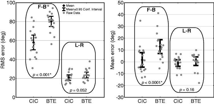
Localization RMS errors (left plot) and mean errors (right plot) in the F–B and L–R dimensions, for the CIC and BTE settings, respectively.

Note. The plots show mean values and 95% confidence intervals, as well as individual data. The indicated p values are according to paired t tests comparing hearing-aid settings within each dimension. CIC = completely-in-the-canal; RMS = root mean square; F–B = front–back; L–R = left–right.

The localization data are generally characterized by a large variation across participants, for example, the F–B RMS errors obtained with the CIC setting ranged from 25° to 83°. The F–B RMS errors (see the left plot in Figure 6) are substantially larger than the L–R RMS errors, indicating that random or systematic reversals are more prominent in the F–B dimension. This observation corresponds well to previous research showing that HI listeners’ localization performance based on monaural pinna cues is generally much poorer than that based on binaural cues, either with (e.g., Keidser et al., 2006, 2009) or without hearing aids (e.g., Noble et al., 1994; Noble, Byrne, & Ter-Horst, 1997). The F–B mean errors (see the right plot in Figure 6) show a trend toward being positive for both microphone settings, although most pronounced for the BTE setting, which means that back-to-front reversals were more common than front-to-back reversals. This finding is in agreement with other data (Best et al., 2010). For both settings, the average L–R mean error was close to 0°, indicating no systematic errors across participants in the L–R dimension.

To compare localization with the two settings, separate analyses (paired t tests) were performed for the two dimensions and the two error measures. In the F–B dimension, the RMS errors were significantly lower with the CIC setting than with the BTE setting (p < .001), with the observed mean difference being 22° (standard deviation = 19°). Of 17 participants, 13 produced a lower F–B RMS error with the CIC setting of at least 15°, while only 1 participant had a lower F–B RMS error with the BTE setting of a similar magnitude. The F–B mean errors also showed a significant mean difference (11°) between settings (p < .0001), with the CIC errors being closest to zero. In the L–R dimension, no significant differences between settings were observed, neither for the RMS errors (3° mean difference, p = .052) nor the mean errors (2° mean difference, p = .16).

Spatial Release From Masking

The individual and average data obtained from the SRM test, that is, the SRT_CO, SRT_F–B, and SRT_L–R, as well as the corresponding values of SRM_F–B and SRM_L–R, for both HA settings, are plotted in Figure 7.

Figure 7.

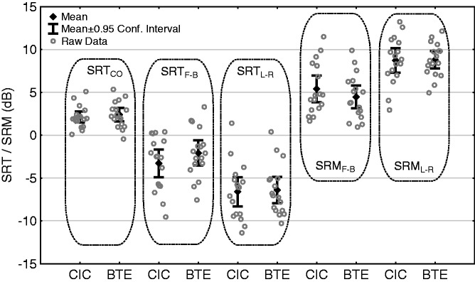
SRTs in the three masking conditions (CO, F–B, and L–R) and the corresponding SRM data in the F–B and L–R masking conditions, for the CIC and BTE settings, respectively.

Note. The plot shows mean values and 95% confidence intervals as well as the individual data. SRM = spatial release from masking; CO = colocated; F–B = front–back; L–R = left–right; CIC = completely-in-the-canal; BTE = behind-the-ear.

Some clear trends can be observed in the SRT data, disregarding the HA settings. Much larger interindividual variation is seen in the SRTs in the two spatially displaced masking conditions than in the SRTs in the colocated masking condition. Furthermore, SRTs are generally highest in the colocated masking condition and lowest in the L–R masking condition, with SRTs in the F–B masking condition being somewhere in between. These trends were also observed in a previous study (Neher et al., 2009) where the same SRM test was used to assess performance with another type of amplification.

The SRM data reflect the trends in the SRT data. That is, SRM was generally higher in the L–R masking condition than in the F–B masking condition, whereas the differences in SRM between HA settings were small in both masking conditions. The mean SRM was 0.9 dB higher (better) with the CIC setting in the F–B condition, whereas it was 0.1 dB lower (worse) with the CIC setting in the L–R condition. A repeated-measures analysis of variance performed on the SRM data with HA setting (CIC/BTE) and masking condition (F–B/L–R) as within-subject factors showed no significant effect of HA setting, F(1, 16) = 0.5, p = .47; a significant effect of masking condition, F(1, 16) = 50.3, p < .00001; and no significant interaction, F(1, 16) = 1.4, p = .25. Thus, the SRM data showed no significant differences between the CIC and BTE settings for any of the masking conditions.

Questionnaire Data

SSQ and SSQ-C

Data from the SSQ and the SSQ-C are reported in the form of the 10 pragmatic subscales developed by Gatehouse & Akeroyd (2006). Table 1 includes the median and the upper and lower quartiles of the SSQ subscale ratings, across participants and HA settings, from the first round of the field test, and similar data for the SSQ-C subscale ratings. In Table 1, the signs of the SSQ-C ratings have been set such that positive ratings indicate a benefit of the CIC setting. The SSQ-C data are also shown for a subgroup consisting of 13 participants because the remaining 4 participants reported that feedback occurred several times daily in the CIC setting. Because the feedback problems may have had a general impact on the SSQ-C ratings, it was decided to recalculate the quartiles of the SSQ-C subscale ratings with the four feedback sufferers excluded.

Table 1.

SSQ and SSQ-C data converted to the pragmatic subscales developed by Gatehouse & Akeroyd (2006).

Subscale label	SSQ (N = 17)	SSQ-C (N = 17)	SSQ-C (N = 13)
Speech in quiet	7.9, 8.6, 9.0	−0.5, 0.0, 1.5	0.0, 0.5, 1.5
Speech in noise	3.8, 5.3, 7.4	−0.5, 0.3, 0.8	0.0, 0.3, 2.5
Speech in speech contexts	5.8, 7.3, 8.2	−0.2, 0.0, 1.0	0.0, 0.0, 2.0
Multiple speech-stream processing and switching	3.0, 5.5, 6.8	0.0, 0.3, 1.3	0.0, 0.7*, 1.5
Localization	8.1, 8.8, 9.0	0.0, 0.0, 0.4	0.0, 0.0, 0.4
Distance and movement	7.9, 8.6, 9.1	0.0, 0.0, 0.1	0.0, 0.0, 0.1
Sound quality and naturalness	8.2, 8.7, 9.3	0.0, 0.0, 0.5	0.0, 0.0, 0.5
Identification of sound and objects	8.6, 9.0, 9.6	0.0, 0.0, 0.2	0.0, 0.0, 0.2
Segregation of sounds	8.7, 9.3, 9.7	0.0, 0.0, 0.5	0.0, 0.0, 0.5
Listening effort	3.7, 6.8, 8.2	−0.5, 0.0, 0.9	−0.1, 0.0, 1.7

Note. The SSQ was used to evaluate the setting used in the first round (on a scale from 0 to 10, where higher is better), whereas the SSQ-C was used to evaluate the difference between the two settings (on a scale from −5 to 5, where positive ratings are in favor of the CIC setting). The 4 participants reporting about frequent feedback problems have been removed from the SSQ-C data shown in the right column. Three quartiles for each subscale with the second quartile (median) in bold are shown. SSQ = Speech, Spatial, and Qualities of Hearing Scale; SSQ-C = Speech, Spatial, and Qualities of Hearing Scale-Comparative; CIC = completely-in-the-canal; BTE = behind-the-ear.

^*Significant benefit of CIC over BTE at p < .05.

Of the 10 SSQ-C subscales, a median rating of zero was observed for eight subscales in the data from all 17 participants, indicating no difference between settings, whereas two subscales had a slightly positive median rating, indicating a benefit of the CIC setting. None of the median values was significantly different from zero according to one-sample Wilcoxon signed-rank tests. The median ratings of zero reflect the fact that many individual ratings of zero were given by the participants. Up to eight ratings of zero on a single subscale were observed. However, among those participants actually stating a preference on those subscales, the trend was a preference for the CIC setting, as indicated by the upper quartiles, which generally were higher than the absolute values of the lower quartiles.

When the four feedback sufferers were excluded from the data analysis, one additional SSQ-C median value became positive, and the median rating of the subscale multiple speech-stream processing and switching now became significantly different from zero (p < .05). The three other speech understanding-related subscales (speech in quiet, speech in noise, and speech in speech contexts) provided p values of .066, .055, and .067, respectively, when testing for deviations from zero. When the items within the speech section of the SSQ-C were analyzed separately, 5 of the 14 items within this section had a positive median value, which was significantly different from zero (p < .05), indicating a benefit of the CIC setting over the BTE setting. Thus, even though the overall trend in the SSQ-C data suggested no difference between the two settings, there were some indications of a preference for the CIC setting in situations involving speech understanding in various contexts. It should be noted that the subscale entitled localization showed no significant difference between settings, with only 6 participants having a positive subscale value (indicating a CIC benefit). This is in contrast to the findings in the localization test described earlier, where a significant benefit of the CIC setting was observed (in the F–B dimension), and where 13 participants showed a CIC RMS-error benefit of at least 15°. It should also be noted that the reported p values were not corrected for multiple comparisons. If the (somewhat conservative) Bonferroni correction had been applied, no significant effects would have remained.

Final preference

The distribution of the participants’ final ratings of preference for the CIC versus BTE settings is shown in Figure 8.

Figure 8.

Distribution of the 17 participants’ final overall preference ratings.

Note. The preferences of the four feedback sufferers are indicated separately.

A total of 12 participants found the CIC setting to be somewhat or much better than the BTE setting, 1 participant had no preference, and a total of 4 participants found the BTE setting to be somewhat or much better than the CIC setting. Thus, the overall trend in the preference ratings was a preference for the CIC setting. This was confirmed by a χ² test in which the distribution of the three overall preference ratings (BTE preference, no preference, and CIC preference) was compared with a pure-chance distribution. The CIC preference was significant (p < .01) both with and without inclusion of the four feedback sufferers in the analysis.

When asked about reasons for their preference, most of the participants stated more than one reason. Among the 12 participants stating a preference for the CIC setting, the most commonly mentioned reasons were related to speech intelligibility (in noise or in groups) and sound quality. There was not any obvious trend in the reasons mentioned by the 4 participants preferring the BTE setting. Acoustic feedback (experienced with the CIC setting) was only mentioned by 1 participant as a specific reason for (strongly) preferring the BTE. In fact, as indicated in Figure 8, two of the four feedback sufferers had a (moderate) overall preference for the CIC setting even though they reported about more feedback problems in that setting.

In the rating of the preference for own versus test hearing aids, 11 participants stated a preference for their own hearing aids, whereas 6 participants stated a preference for the (preferred setting of the) test hearing aids. Thus, the general trend was a preference for the participants’ own hearing aids. The preference was significant (p < .01) according to a χ² test conducted in the same way as in the analysis of the CIC versus BTE preference ratings. The main reasons for preferring the own hearing aids over the test hearing aids were related to the physical fit, the cosmetic appearance, and the acoustic feedback issues experienced with the experimental hearing aid. With most of the participants being used to open BTE fittings (with soft earmolds and no feedback issues), these findings were not surprising.

Correlations Between Outcome Measures

The correlations between preference ratings and objectively and subjectively measured differences between HA settings were calculated using the Spearman’s rank correlation coefficient (r_s). For the localization (RMS error) and SRM data, the differences between CIC and BTE settings were calculated in the L–R and F–B dimension, respectively, with positive values indicating benefits of the CIC setting. The three SSQ-C section mean ratings represented the subjectively measured data. Thus, seven correlation coefficients were calculated. When testing for significance, a Bonferroni correction was applied, which changed the significance level from .05 to .007. The correlations between localization improvements and preference ratings were small, abs(r_s) < .2, and nonsignificant (p > .5). The correlations between SRM improvements and preference rating were .50 for the L–R dimension and .13 for the F–B dimension. Even though neither of these correlations was significant at the Bonferroni-corrected level of .007 (p = .04 and p = .61, respectively), it is noteworthy that the correlation between preference and L–R improvement was substantially stronger than the correlation between preference and F–B improvement. The preference ratings were significantly correlated with the SSQ-C speech mean rating (r_s = .68, p < .007) and qualities mean rating (r_s = .63, p < .007), but not with the spatial mean rating (r_s = .55, p = .02).

The intercorrelations among the measured differences between HA settings in the different outcome domains (localization, SRM, and SSQ-C) were also calculated. However, none of the correlation coefficients were significant at p = .05. This finding reflects a somewhat mixed picture across the different outcome measures. Only 2 of the 17 participants showed consistent benefit from and preference for the CIC setting over the BTE setting on the outcome measures. The remaining participants had inconsistent benefit patterns, showing a CIC benefit on some outcome measures and a BTE benefit (or no difference) on others.

Discussion

Localization

The results from the localization test showed a significant benefit for the CIC setting over the BTE setting in the F–B dimension, with an observed mean RMS error improvement of 22°. On an individual level, a CIC benefit was observed for 15 of the 17 participants. The observed CIC benefit ranged from 1° to 52°, and it exceeded 15° for 13 of the participants. It should be noted that level roving was applied to the stimuli used in the localization test in the present study. Therefore, the observed difference between the settings in the F–B dimension cannot be explained by level cues, which have been used to explain (part of) the differences between ITE and BTE hearing aids observed in other studies (e.g., Byrne & Noble, 1998). In the L–R dimension, no significant localization difference between settings was observed. This was also according to expectations because both settings provided binaural spatial cues (ILDs and ITDs) to the participants in this dimension. As mentioned in the Experimental Hearing Aids section, differences in the disruption of these cues between the two settings were not expected. All in all, the localization results are in agreement with expectations and the results obtained in previous comparisons of hearing aids with microphone positions above the ear and at the entrance to the ear canal, respectively (Best et al., 2010; Orton & Preves, 1979; Türk, 1986; Van den Bogaert et al., 2011; Westermann & Tøpholm, 1985).

Besides microphone positioning, hearing aids offer other means of providing monaural spatial cues and thereby changing the users’ localization abilities in the F–B dimension. Therefore, it seems reasonable to discuss whether the localization benefit observed for the CIC setting (i.e., the benefit of preserving pinna cues) in the F–B dimension could have been obtained in other ways.

Modern BTE hearing aids often include directionality, for example, as an adaptive feature or as a second program in the hearing aid. The effect of adding directionality was not investigated in the present study, but in a study on HI listeners, Keidser et al. (2009) investigated the effects of different directional BTE HA microphone patterns on localization in the horizontal plane, with 3 weeks of acclimatization to each microphone pattern before the testing was carried out. They used stimuli with a variety of spectral characteristics. They found that F–B localization depended on microphone pattern and type of stimulus. The largest improvement in F–B RMS error relative to an omnidirectional pattern was obtained with a microphone pattern offering partial directionality (above 1 kHz) and using a cockatoo stimulus with high-frequency emphasis. In that case, the mean F–B RMS error was reduced from approximately 68° to approximately 55°. Directional patterns with full directionality or with directionality above 2 kHz showed smaller improvements relative to the omnidirectional pattern, and the improvements were smaller or nonexisting for stimuli with fewer high-frequency contents. Thus, disregarding some differences in test procedures between the studies, the average benefit in F–B RMS error of the CIC setting in the present study (22°) was larger than the largest benefit of directionality (13°) observed by Keidser et al. This indicates that a localization benefit may be provided by a CIC microphone position, which exceeds the benefit obtainable with a directional HA microphone. However, when individual variations in the data are taken into account, it must also be realized that some HA users may obtain (at least) the same localization benefit from a directional microphone in a BTE position as they do from an omnidirectional microphone in a CIC position. This is supported by Van den Bogaert et al. (2011), who found the F–B localization performance with a BTE hearing aid equipped with a fixed directional microphone to be just as good as the localization performance with an ITC hearing aid, using a broadband signal as stimulus.

Spatial Release From Masking

The SRM results showed no significant differences between the CIC and BTE settings in either the L–R or the F–B masking condition of the test. The lack of a difference was expected in the L–R masking condition, where the participants had access to binaural spatial cues with both settings. This access also explains the overall improvement in performance from the F–B to the L–R masking condition. However, in the F–B masking condition, the preservation of pinna cues in the CIC setting was expected to result in a spatial-unmasking benefit over the BTE setting. The observed mean benefit on SRT_F–B of approximately 1.2 dB was actually smaller than the benefit expected due to the acoustic shadow effect of the pinna alone, which has been estimated to be approximately 3 dB (Freyman et al., 2005).

The fact that no CIC benefit was observed in the F–B spatial-unmasking task while a significant CIC benefit was observed in the F–B localization task may suggest that different cues are important for the SRM and localization tasks. In particular, the data indicate that the spectral pinna cues are more important for F–B localization than for F–B spatial unmasking. This is also suggested by Hawley, Litovsky, and Colburn (1999) who found little correspondence between differences in localization performance and differences in speech-intelligibility (in noise) performance when free-field listening was compared with binaural and monaural listening in an HRTF-based virtual environment. This is in line with the findings from the present study where no correlation between the spatial-unmasking benefit and the localization benefit was found in either the L–R dimension or the F–B dimension. However, the HRTFs used in Hawley et al.’s study were not personalized, and the participants were offered no time for acclimatization, which the authors suggest could affect some of their observations. This is in contrast to the present study, which focused on providing personalized spectral cues with appropriate time for acclimatization. Furthermore, an actual F–B test condition was not included in their experiments, which only included target and masker positions in front and to the side of the participants.

Another possible explanation for the observed lack of F–B unmasking benefit in the present study may be that the SRM test was unable to detect the F–B spatial-unmasking effect of preserving pinna cues. The difference between the F–B and the L–R conditions is access (or not) to binaural cues, which have been found to be potent for improving speech intelligibility (e.g., Neher et al., 2009), and rather robust to deviations from exact representation (Hawley et al., 1999). In contrast, pinna cues are much more subtle spectral changes at high frequencies, and we will argue that the percept required to perform F–B spatial unmasking is much more fragile and more difficult to access than the percept required to perform L–R spatial unmasking. Thus, although the spatial-unmasking test was able to detect distinct differences, for example, access (or not) to binaural cues, it may have been unable to detect the more subtle differences caused by access (or not) to pinna cues. The different robustness of binaural cues and pinna cues may also explain the observation that the overall preference rating showed a stronger correlation with the L–R SRM improvement (with the CIC setting) than with the F–B SRM improvement.

Questionnaires

One thing that was noteworthy about the SSQ data on the setting used in the first round of the field test was that the median SSQ subscale ratings, across the two HA settings, generally were quite high. When comparing with other available SSQ data about aided performance (e.g., Gatehouse & Akeroyd, 2006; Keidser et al., 2009), the ratings obtained in the present study were generally similar to or above the ratings obtained in other studies. This indicates that the participants in general were satisfied with the experimental hearing aids, and that no serious systematic (performance-degrading) problems occurred.

The SSQ-C data from all 17 participants indicated a minor advantage for the CIC setting, but the difference was not significant on any of the 10 pragmatic subscales used in the analysis. However, exclusion of the four feedback sufferers led to a more pronounced general CIC benefit, with one subscale (and five individual items) within the speech section of the SSQ-C showing a significant difference between settings. This finding is backed up by the general preference for the CIC setting, which was expressed by a majority of the participants, as well as by the stated reasons for their preference. The fact that it was SSQ-C items on speech intelligibility in different contexts that showed a benefit of the CIC, while the spatial subscales (i.e., localization and distance and movement) showed no differences, may be a bit surprising because it is contrary to the results from the laboratory tests. However, this finding may reflect that HA users in real life are more concerned about understanding speech than localizing sound.

Regarding the mismatch between the localization benefit of the CIC setting found in the laboratory and the lack of real-life benefit reported by the participants, this is in agreement with results obtained by Keidser et al. (2009). In a localization test, they found differences between different HA microphone configurations, but no differences were found by means of the SSQ when the same configurations were evaluated in real life. Keidser et al. speculated that the 3-week acclimatization period used in their study was too short to reveal any differences in real-world localization abilities. This could also have been an issue in the present study where the acclimatization period was of the same magnitude (although 1–2 weeks longer). Furthermore, it could be questioned whether the possibly small contrasts between settings could be memorized by the participants when filling in the SSQ-C around 1 month after using the first setting of the hearing aids. This aspect of using the SSQ-C remains to be investigated.

Another possible explanation for the mismatch between the laboratory and real-life measures may be that the laboratory test does not offer a very good representation of the situations encountered by the participants in real life, where meaningful visual cues and head movements can be used (as opposed to the test used in the present study). From that perspective, the lack of correspondence between laboratory and subjective data may not be surprising. This is in agreement with Byrne et al. (1992), who found no difference in performance between ITE and BTE hearing aids in a laboratory setup where head movements were allowed. Conversely, it could also be argued that none of the items in the SSQ-C may be suitable for tapping into the very specific laboratory condition where a significant benefit of the CIC setting was observed. In particular, this relates to the F–B test condition, which in its pure form may be rarely encountered in real-life situations. The experience with directional microphones evaluated in the laboratory versus real life reported by Cord et al. (2002) suggests that, had the participants been urged to seek out resembling situations in their everyday life, they would perhaps have been more likely to perceive a real-life localization benefit.

Conclusion

The localization experiment showed that preserving pinna cues, by moving the microphone from above the ear to within the concha of the ear, leads, on average, to a significant improvement in localization performance in the F–B dimension. The mean RMS error was reduced by 22° with the pinna cue-preserving CIC setting in comparison with the BTE setting, which did not preserve these cues. No difference between settings was observed in the L–R dimension, in agreement with the basic hypothesis of the study and previous findings. However, there was no correspondence between the CIC localization benefit obtained in the laboratory and the reported real-life experience, where no significant mean CIC localization benefit was observed, and where an individual benefit was reported by only 6 participants as opposed to the 13 participants showing a real benefit in the laboratory. The spatial-unmasking test showed no significant effect of providing pinna cues in either the F–B or the L–R dimension, and the hypothesis that preservation of pinna cues provides a spatial-unmasking benefit could not be confirmed. There was a significant overall preference for the CIC setting, but only 2 of the 17 participants showed a consistent benefit from and preference for the CIC setting on all the outcome measures, where the preservation of pinna cues was expected to provide a benefit. The implication of these results for clinical HA fittings is that pinna cue-preserving HA fittings (e.g., fittings based on a CIC microphone position) at best will offer benefit to some users in specific real-life situations and that they do not significantly disadvantage anyone.

Declaration of Conflicting Interests

The authors declared no potential conflicts of interest with respect to the research, authorship, and/or publication of this article.

Funding

The authors received no financial support for the research, authorship, and/or publication of this article.

Authors’ Note

The data from this study were presented orally in preliminary form at the International Hearing Aid Research Conference (IHCON), Lake Tahoe, CA, USA, August 11–15, 2010.

Tobias Neher is now at Cluster of Excellence “Hearing4all,” Medical Physics Group, Department of Medical Physics and Acoustics, Carl-von-Ossietzky Universität, Oldenburg, Germany; and René Burmand Johannesson is now at Phonak AG, Stäfa, Switzerland.

References

- Asano F., Suzuki Y., Sone T. (1990) Role of spectral cues in median plane localization. Journal of the Acoustical Society of America 88: 159–168 [DOI] [PubMed] [Google Scholar]
- Best, V., Kalluri, S., McLachlan, S., Valentine, S., Edwards, B., & Carlile, S. (2010). A comparison of CIC and BTE hearing aids for three-dimensional localization of speech. International Journal of Audiology, 49, 723–732. [DOI] [PubMed]
- Blauert J. (1997) Spatial hearing: The psychophysics of human sound localization, Cambridge, MA: MIT Press [Google Scholar]
- Brand T., Kollmeier B. (2002) Efficient adaptive procedures for threshold and concurrent slope estimates for psychophysics and speech intelligibility tests. Journal of the Acoustical Society of America 111: 2801–2810 [DOI] [PubMed] [Google Scholar]
- Bronkhorst A. W. (2000) The cocktail party phenomenon: A review of research on speech intelligibility in multiple-talker conditions. Acta Acustica United With Acustica 86: 117–128 [Google Scholar]
- Butler R. A. (1986) The bandwidth effect on monaural and binaural localization. Hearing Research 21: 67–73 [DOI] [PubMed] [Google Scholar]
- Byrne D., Noble W. (1998) Optimizing sound localization with hearing aids. Trends in Amplification 3: 51–73 [DOI] [PMC free article] [PubMed] [Google Scholar]
- Byrne D., Noble W., Lepage B. (1992) Effects of long-term bilateral and unilateral fitting of different hearing aid types on the ability to locate sounds. Journal of the American Academy of Audiology 3: 369–382 [PubMed] [Google Scholar]
- Cord M. T., Surr R. K., Walden B. E., Olson L. (2002) Performance of directional microphone hearing aids in everyday life. Journal of the American Academy of Audiology 13: 295–307 [PubMed] [Google Scholar]
- Cox R. M., Moore J. N. (1988) Composite speech spectrum for hearing and gain prescriptions. Journal of Speech and Hearing Research 31: 102–107 [DOI] [PubMed] [Google Scholar]
- Flynn M. (2003) Opening ears: The scientific basis for an open ear acoustic system. Hearing Review 10: 34–37, 67 [Google Scholar]
- Freyman R. L., Helfer K. S., Balakrishnan U. (2005) Spatial and spectral factors in release from informational masking in speech recognition. Acta Acustica United With Acustica 91: 537–545 [Google Scholar]
- Freyman R. L., Helfer K. S., McCall D. D., Clifton R. K. (1999) The role of perceived spatial separation in the unmasking of speech. Journal of the Acoustical Society of America 106: 3578–3588 [DOI] [PubMed] [Google Scholar]
- Gatehouse S., Akeroyd M. (2006) Two-eared listening in dynamic situations. International Journal of Audiology 45(Suppl. 1): S120–S124 [DOI] [PubMed] [Google Scholar]
- Gatehouse S., Noble W. (2004) The Speech, Spatial and Qualities of Hearing Scale (SSQ). International Journal of Audiology 43: 85–99 [DOI] [PMC free article] [PubMed] [Google Scholar]
- Good M. D., Gilkey R. H. (1996) Sound localization in noise: The effect of signal-to-noise ratio. Journal of the Acoustical Society of America 99: 1108–1117 [DOI] [PubMed] [Google Scholar]
- Hammershøi D., Møller H. (1996) Sound transmission to and within the human ear canal. Journal of the Acoustical Society of America 100: 408–427 [DOI] [PubMed] [Google Scholar]
- Hartmann W. M., Rakerd B., Gaalaas J. B. (1998) On the source-identification method. Journal of the Acoustical Society of America 104: 3546–3557 [DOI] [PubMed] [Google Scholar]
- Häusler R., Colburn S., Marr E. (1983) Sound localization in subjects with impaired hearing. Spatial-discrimination and interaural-discrimination tests. Acta Otolaryngologica Supplementum 96(400): 1–62 Retrieved from http://informahealthcare.com/doi/abs/10.3109/00016488309105590 [DOI] [PubMed] [Google Scholar]
- Hawley M. L., Litovsky R. Y., Colburn H. S. (1999) Speech intelligibility and localization in a multi-source environment. Journal of the Acoustical Society of America 105: 3436–3448 [DOI] [PubMed] [Google Scholar]
- IEC 60118-8. (2005). Electroacoustics Hearing aids Part 8: Methods of measurement of performance characteristics of hearing aids under simulated in situ working conditions. Geneva, Switzerland: International Electrotechnical Commission.
- Jensen, N. S., Akeroyd, M., Noble, W., & Naylor, G. (2009, October). The Speech, Spatial and Qualities of Hearing scale (SSQ) as a benefit measure. Poster presented at the 4th International NCRAR conference, Portland, OR.
- Keidser G., O’Brien A., Hain J. U., McLelland M., Yeend I. (2009) The effect of frequency-dependent microphone directionality on horizontal localization performance in hearing-aid users. International Journal of Audiology 48: 789–803 [DOI] [PubMed] [Google Scholar]
- Keidser G., Rohrseitz K., Dillon H., Hamacher V., Carter L., Rass U., Convery E. (2006) The effect of multi-channel wide dynamic range compression, noise reduction, and the directional microphone on horizontal localization performance in hearing aid wearers. International Journal of Audiology 45: 563–579 [DOI] [PubMed] [Google Scholar]
- Leeuw A. R., Dreschler W. A. (1987) Speech understanding and directional hearing for hearing-impaired subjects with in-the-ear and behind-the-ear hearing aids. Scandinavian Audiology 16: 31–36 [DOI] [PubMed] [Google Scholar]
- Lorenzi C., Gatehouse S., Lever C. (1999) Sound localization in noise in hearing-impaired listeners. Journal of the Acoustical Society of America 105: 3454–3463 [DOI] [PubMed] [Google Scholar]
- Mehrgardt S., Mellert V. (1977) Transformation characteristics of the external human ear. Journal of the Acoustical Society of America 61: 1567–1576 [DOI] [PubMed] [Google Scholar]
- Moore B. C., Stone M. A., Fullgrabe C., Glasberg B. R., Puria S. (2008) Spectro-temporal characteristics of speech at high frequencies, and the potential for restoration of audibility to people with mild-to-moderate hearing loss. Ear and Hearing 29: 907–922 [DOI] [PMC free article] [PubMed] [Google Scholar]
- MRC Institute of Hearing Research. (2012). IHR products: Questionnaires available for downloads. Retrieved from http://www.ihr.mrc.ac.uk/index.php/products/display/questionnaires.
- Musicant A. D., Butler R. A. (1984) The influence of pinnae-based spectral cues on sound localization. Journal of the Acoustical Society of America 75: 1195–1200 [DOI] [PubMed] [Google Scholar]
- Neher T., Behrens T., Carlile S., Jin C., Kragelund L., Petersen A. S., Schaik A. (2009) Benefit from spatial separation of multiple talkers in bilateral hearing-aid users: Effects of hearing loss, age, and cognition. International Journal of Audiology 48: 758–774 [DOI] [PubMed] [Google Scholar]
- Neher, T., Behrens, T., Kragelund, L., & Petersen, A. S. (2008). Spatial unmasking in aided hearing-impaired listeners and the need for training. In T. Dau et al. (Eds.), Auditory signal processing in hearing-impaired listeners (pp. 515–522). Copenhagen, Denmark: Centertryk A/S.
- Neher T., Laugesen S., Jensen N. S., Kragelund L. (2011) Can basic auditory and cognitive measures predict hearing-impaired listeners’ localization and spatial speech recognition abilities? Journal of the Acoustical Society of America 130: 1542–1558 [DOI] [PubMed] [Google Scholar]
- Noble W., Byrne D., LePage B. (1994) Effects on sound localization of configuration and type of hearing impairment. Journal of the Acoustical Society of America 95: 992–1005 [DOI] [PubMed] [Google Scholar]
- Noble W., Byrne D., Ter-Horst K. (1997) Auditory localization, detection of spatial separateness, and speech hearing in noise by hearing impaired listeners. Journal of the Acoustical Society of America 102: 2343–2352 [DOI] [PubMed] [Google Scholar]
- Orton J. F., Preves D. A. (1979) Localization ability as a function of hearing aid microphone placement. Hearing Instruments 30: 18–21 [Google Scholar]
- Rakerd B., Vander Velde T. J., Hartmann W. M. (1998) Sound localization in the median sagittal plane by listeners with presbyacusis. Journal of the American Academy of Audiology 9: 466–479 [PubMed] [Google Scholar]
- Rychtáriková M., Van den Bogaert T., Vermeir G., Wouters J. (2011) Perceptual validation of virtual room acoustics: Sound localisation and speech understanding. Applied Acoustics 72: 196–204 [Google Scholar]
- Singh G., Pichora-Fuller M. K. (2010) Older adults’ performance on the Speech, Spatial, and Qualities of Hearing Scale (SSQ): Test-retest reliability and a comparison of interview and self-administration methods. International Journal of Audiology 49: 733–740 [DOI] [PubMed] [Google Scholar]
- Supin A. Y., Popov V. V., Milekhina O. N., Tarakanov M. B. (1994) Frequency resolving power measured by rippled noise. Hearing Research 78: 31–40 [DOI] [PubMed] [Google Scholar]
- Türk R. (1986) A clinical comparison between behind-the-ear and in-the-ear hearing aids. Audiological Acoustics 25: 78–86 [Google Scholar]
- Van den Bogaert, T., Carette, E., & Wouters, J. (2009). Sound localization with and without hearing aids. In M. M. Boone (Ed.), NAG-DAGA International Conference on Acoustics (pp. 1314–1317). Red Hook, NY: Curran Associates.
- Van den Bogaert T., Carette E., Wouters J. (2011) Sound source localization using hearing aids with microphones placed behind-the-ear, in-the-canal, and in-the-pinna. International Journal of Audiology 50: 164–176 [DOI] [PubMed] [Google Scholar]
- Van den Bogaert T., Klasen T. J., Moonen M., Van Deun L., Wouters J. (2006) Horizontal localization with bilateral hearing aids: Without is better than with. Journal of the Acoustical Society of America 119: 515–526 [DOI] [PubMed] [Google Scholar]
- Wagener K., Josvassen J. L., Ardenkjaer R. (2003) Design, optimization and evaluation of a Danish sentence test in noise. International Journal of Audiology 42: 10–17 [DOI] [PubMed] [Google Scholar]
- Walden B. E., Surr R. K., Cord M. T., Edwards B., Olson L. (2000) Comparison of benefits provided by different hearing aid technologies. Journal of the American Academy of Audiology 11: 540–560 [PubMed] [Google Scholar]
- Westermann S., Tøpholm J. (1985) Comparing BTEs and ITEs for localizing speech. Hearing Instruments 36: 20–24, 36 [Google Scholar]
- Zurek P. (1993) Binaural advantages and directional effects in speech intelligibility. In: Studebaker G. A., Hockberg I. (ed.) Acoustical factors affecting hearing aid performance, Needham Heights, MA: Allyn and Bacon, pp. 225–276 [Google Scholar]