A Graphical Model for Estimating Stimulus-Evoked Brain Responses from Magnetoencephalography Data with Large Background Brain Activity

Abstract

This paper formulates a novel probabilistic graphical model for noisy stimulus-evoked MEG and EEG sensor data obtained in the presence of large background brain activity. The model describes the observed data in terms of unobserved evoked and background factors with additive sensor noise. We present an Expectation-Maximization (EM) algorithm that estimates the model parameters from data. Using the model, the algorithm cleans the stimulus-evoked data by removing interference from background factors and noise artifacts, and separates those data into contributions from independent factors. We demonstrate on real and simulated data that the algorithm outperforms benchmark methods for denoising and separation. We also show that the algorithm improves the performance of localization with beamforming algorithms.

1 Introduction

Electromagnetic source imaging (ESI), the reconstruction of the spatiotemporal activation of brain sources from MEG and EEG data, is increasingly being used in numerous studies of human cognition in both normals and in various clinical populations [14, 2, 13]. The major advantage of ESI over other noninvasive functional brain imaging techniques is the ability to obtain valuable information about neural dynamics with high temporal resolution on the order of milliseconds. A major problem in ESI is that MEG and EEG measurements, which use sensors located outside the brain, generally contain not only signals associated with brain sources of interest, but also signals from other sources such as spontaneous brain activity, eye blinks and other biological and non-biological sources of artifacts. Interference signals from these sources overlap spatially and temporally with those from the brain sources of interest, making it difficult to obtain accurate reconstructions.

Many approaches have been taken to address the problems of reducing noise from artifacts, and from interference signals due to background brain activity, with varying degress of success. First, event related averaging of multiple trials may be used to reduce the contributions from non stimulus-locked and non phase-locked activity. Averaging reduces the contribution of background brain activity on the order of the square root of the number of trials. This is often performed after rejection of manually-selected trials that contain conspicuous artifacts, such as eyeblinks or saccades. However, averaging and manual trial segment rejection require that the data be collected for a large number of trials, which effectively limits the number of stimulus conditions in a particular experiment.

Second, model-based approaches have been used to either model the neural generator [9, 7, 6, 3], or to model artifacts[5]. The former involves defining a parametric model for the event-related brain response and the background noise and estimating parameters using a maximum-likelihood methods. The latter involves denoising of the data by identifying and removing portions of data that fit to previously estimated models of an array of artifacts. With the latter technique only irregularities that have been previously identified and modeled well can be removed.

Third, data driven approaches such as Principal Component Analysis (PCA), Wiener filtering and matched filtering and, more recently, Independent Components Analysis (ICA), have been used for denoising and artifact rejection [10, 11, 12, 21, 23, 34, 19, 15, 22, 32, 27, 16, 20, 18].These approaches have provided some benefits but require a subjective choice of many parameters such as dimensionality, thresholds and component selection. Most of these methods usually don't work well for low SNR and are computationally prohibitive for multichannel systems with large number of channels. Furthermore, most of these algorithms also provide no principled mechanism for model order selection. Hence, the selection of the number of spatially distinct evoked sources and the number of sources of interest must be based on ad-hoc methods or by expert analysis.

In this paper we present a novel and powerful approach for the suppression of interference signals and the separation of signals from individual evoked sources. This approach is formulated in the framework of probabilistic graphical models with latent variables, which has been developed and studied in the fields of machine learning and statistics [17]. In the graphical modeling framework, observed data are modeled in terms of a set of latent variables, which are signals that are not directly observable. The dependence of the data on the latent variables is specified by a parameterized probability distribution. The latent variables are modeled by their own probability distribution. The combined distributions define a probabilistic model for the observed data. The model parameters are inferred from data using an expectation-maximization (EM) type algorithm, which is a standard technique for performing maximum likelihood in latent variable models. Problems such as interference suppression and source separation then translate to the problem of probabilistic (Bayesian) inference of appropriate latent variables.

In our case, stimulus-evoked MEG and EEG data are modeled using a new probabilistic graphical model, which is based on the well known factor analysis model [26], and on its extension, independent factor analysis [1]. The new model is termed stimulus evoked independent factor analysis (SEIFA). This model describes the observed data in terms of two sets of independent latent variables, termed factors. The factors in the first set represent evoked sources, and the factors in the second set represent interference sources. The sensor data are generated by linearly combining the factors in the two sets using two mixing matrices, followed by adding sensor noise. The mixing matrices and the precision matrix of the sensor noise constitute the SEIFA model parameters. The interference mixing matrix (the one applied to the interference factors) and the noise precision are inferred from pre-stimulus data, whereas the evoked mixing matrix is inferred from the post-stimulus data.

The paper is organized as follows. The SEIFA probabilistic graphical is defined in mathematical terms in section II. Section III presents a VB-EM (a generalization of standard expectation maximization) algorithm [25, 1] for inferring this model from data. Section IV provides an estimator for the clean evoked response, i.e., the contribution of the evoked factors alone to the sensor data, using the model to remove the contribution of the interference sources. It also breaks this estimator into the separate contributions from each independent evoked factor. Moreover, this section presents an automatically regularized estimator of the correlation matrix of the clean evoked response, as well as the correlation matrix of the separate contribution from each evoked factor. Section V demonstrates, using real and simulated data, that the algorithm provides interference-robust estimates of the time course of the stimulus evoked response. Furthermore, it shows that using the regularized evoked covariance in an existing source localization method improves the performance of that method. Section VI concludes with a discussion of our results and of extensions to the SEIFA framework.

2 SEIFA Probabilistic Graphical Model

This section presents the SEIFA probabilistic graphical model, which is the focus of this paper. The SEIFA model describes observed MEG and EEG sensor data in terms of three types of underlying, unobserved signals: (1) signals arising from stimulus evoked sources, (2) signals arising from interference sources, and (2) sensor noise signals. The model is inferred from data by an algorithm presented in the next section. Following inference, the model is used to separate the evoked source signals from those of the interference sources and from sensor noise, thus providing a clean version of the evoked response. The model further separates the evoked response into statistically independent factors. In addition, it produces a regularized correlation matrix of the clean evoked response and of each independent factors, which facilitates localization.

Let y_in denote the signal recorded by sensor i = 1 : K at time n = 1 : N. We assume that these signals arise from L evoked factors and M interference factors that are combined linearly. Let x_jn denote the signal of evoked factor j = 1 : L, and let u_jn denote the signal of interference factor j = 1 : M, both at time n. We use the term factor rather than source for a reason explained below. Let A_ij denote the evoked mixing matrix, and let B_ij denote the interference mixing matrix. Those matrices contain the coefficients of the linear combination of the factors that produces the data. They are analogous to the factor loading matrix in the factor analysis model. Let v_in denote the noise signal on sensor i. Mathematically,

$$y_{\mathit{\text{in}}}=\sum _{j=1}^L{A}_{\mathit{\text{ij}}}{x}_{\mathit{\text{jn}}}+\sum _{j=1}^M{B}_{\mathit{\text{ij}}}{u}_{\mathit{\text{jn}}}+v_{\mathit{\text{in}}}$$ (1)

We use an evoked stimulus paradigm, where a stimulus is presented at a specific time, termed the stimulus onset time, and is absent beforehand. The stimulus onset time is defined as n = N₀ + 1. The period preceding the onset n = 1 : N₀ is termed pre-stimulus period, and the period following the onset n = N₀ + 1 : N is termed post-stimulus period. We assume the evoked factors are active only post stimulus and satisfy x_jn = 0 before its onset. Hence

$$y_n=\{\begin{array}{ll}{\mathit{\text{Bu}}}_n+v_n,\hfill & n=1:N_0\hfill \\ {\mathit{\text{Ax}}}_n+{\mathit{\text{Bu}}}_n+v_n,\hfill & n=N_0+1:N\hfill \end{array}$$ (2)

To turn (2) into a probabilistic model, each signal must be modelled by a probability distribution. Here, each evoked factor is modelled by a mixture of Gaussian (MOG) distributions. For factor j we have a MOG model with S_j components, also termed states

$$p(x_{\mathit{\text{jn}}})=\sum _{s_j=1}^{S_j}\mathcal{N}(x_{\mathit{\text{jn}}}|{\mu }_{j,s_j},{\nu }_{j,s_j}){\pi }_{j,s_j}$$ (3)

State s_j is a Gaussian¹ with mean μ_j,sj and precision ν_j,sj, and its probability is π_j,sj. We model the factors as mutually statistically independent, hence

$$p(x_n)=\prod _{j=1}^{L}p(x_{\mathit{\text{jn}}})$$ (4)

There are two reasons for using MOG distributions, rather than Gaussians, to describe the evoked factors. First, evoked brain sources are often characterized by spikes or by modulated harmonic functions, leading to non-Gaussian distributions. Second, previous work on ICA has shown that independent Gaussian sources that are linearly mixed cannot be separated. Since we aim to separate the evoked response into contributions from individual factors, we must therefore use independent non-Gaussian factor distributions. Third, as is well known, a MOG model with a suitably chosen number of states can describe arbitrary distributions at the desired level of accuracy.

For interference signals and sensor noise we employ a Gaussian model. Each interference factor is modelled by a zero-mean Gaussian distribution with unit precision, p(u_jn) = ( (u_jn | 0, 1). SEIFA describes the factors as independent,

$$p(u_n)=\prod _{j=1}^M\mathcal{N}(u_{\mathit{\text{jn}}})=\mathcal{N}(u_n|0,I)$$ (5)

The Gaussian model implies that we exploit only second order statistics of the interference signals. This contrasts with the evoked signals, whose MOG model facilitates exploiting higher order statistics, leading to more accurate reconstruction and to separation.

The sensor noise is modelled by a zero-mean Gaussian distribution with a diagonal precision matrix λ,

$$p(v_n)=\mathcal{N}(v_n|0,\mathrm{\lambda })$$ (6)

From (2) we obtain p(y_n | x_n, u_n) = p(υ_n) where we substitute υ_n = y_n − Ax_n − Bu_n with x_n = 0 for n = 1 : N₀. Hence, we obtain the distribution of the sensor signals conditioned on the evoked and interference factors,

$$p(y_n|x_n,u_n,A,B)=\{\begin{array}{ll}\mathcal{N}(y_n|{\mathit{\text{Bu}}}_n,\mathrm{\lambda }),\hfill & n=1:N_0\hfill \\ \mathcal{N}(y_n|{\mathit{\text{Ax}}}_n+{\mathit{\text{Bu}}}_n,\mathrm{\lambda }),\hfill & n=N_0+1:N\hfill \end{array}$$ (7)

SEIFA also makes an i.i.d. assumption, meaning the signals at different time points are independent. Hence

$$\begin{array}{lll}p(y|x,u,A,B)\hfill & =\hfill & \prod _{n=1}^{N}p(y_n|x_n,u_n,A,B)\hfill \\ \hfill p(x)& =\hfill & \prod _{n=N_0+1}^{N}p(x_n)\hfill \\ \hfill p(u)& =\hfill & \prod _{n=1}^{N}p(u_n)\hfill \end{array}$$ (8)

where y, x, u denote collectively the signals y_n, x_n, u_n at all time points. The i.i.d. assumption is made for simplicity, and implies that the algorithm presented below can exploit the spatial statistics of the data but not their temporal statistics.

To complete the definition of SEIFA, we must specify prior distributions over the model parameters. For the noise precision matrix λ we choose a flat prior, p(λ) = const. For the mixing matrices A, B we use a conjugate prior. A prior distribution is termed conjugate w.r.t. a model when its functional form is identical to that of the posterior distribution (see the discussion below Eq. (58)). We choose a prior where all matrix elements are independent zero-mean Gaussians

$$\begin{array}{lll}p(A)\hfill & =\hfill & \prod _{\mathit{\text{ij}}}\mathcal{N}(A_{\mathit{\text{ij}}}|0,{\mathrm{\lambda }}_i{\alpha }_j)\hfill \\ p(B)\hfill & =\hfill & \prod _{\mathit{\text{ij}}}\mathcal{N}(B_{\mathit{\text{ij}}}|0,{\mathrm{\lambda }}_i{\beta }_j)\hfill \end{array}$$ (9)

and the precision of the ijth matrix element is proportional to the noise precision λ_i on sensor i. It is the λ dependence which makes this prior conjugate. (It can be shown that in the limit of zero sensor noise, λ → ∞, the impact of the prior on the posterior mean of A, B would vanish in the absence of this dependence, which would be undesirable.) The proportionality constants α_j and β_j constitute the parameters of the prior, also known as (aka) hyperparameters. Eqs. (8,9) together with Eqs. (4,5,7) fully define the SEIFA model.

3 Inferring the SEIFA Model from Data: A VB-EM Algorithm

This section presents an algorithm that infers the SEIFA model from data. SEIFA is a probabilistic model with latent variables, since the evoked and interference factors are not directly observable. We use an extended version of the expectation maximization (EM) algorithm to infer the model from data. This version is termed variational Bayesian EM (VB-EM).

Standard EM computes the most likely parameter value given the observed data, aka the maximum aposteriori (MAP) estimate. In contrast, VB-EM considers all possible parameters values, and computes the probability of each value conditioned on the observed data. VB-EM therefore treats latent variables and parameters on equal footing by computing posterior distributions for both quantities. One may, however, choose to compute a posterior only over one set of model parameters, while computing just a MAP estimate for the other set.

VB-EM is an iterative algorithm, where each iteration consists of an E-step and an M-step. The E-step computes the sufficient statistics (SS) of the latent variables, and the M-step computes the SS of the parameters. (SS of an unobserved variable are quantities that define its posterior distribution.) The algorithm is iterated to convergence, which is guaranteed.

The VB-EM algorithm has several advantages compared to standard EM. It is more robust to overfitting, which can be a significant problem when working with high-dimensional but relatively short time series, as we do in this paper. It produces automatically regularized estimators, such as for the evoked response correlation matrix, where standard EM produces poorly conditioned ones. In addition, the variance of posterior distribution it computes (essentially the estimator's variance, or squared error) provides a measure of the range of parameter values compatible with the data.

We now describe the VB-EM algorithm for the SEIFA model. A full derivation is provided in the Appendix.

3.1 E-step

The E-step of VB-EM computes the SS for the latent variables conditioned on the data. For the pre-stimulus period, n = 1 : N₀, the latent variables are the interference factors u_n. Compute their posterior mean ū_n and covariance Φ by

$$\begin{array}{lll}{\overline{u}}_n\hfill & =\hfill & \mathrm{\Phi }{\overline{B}}^T\mathrm{\lambda }{y}_n\hfill \\ \mathrm{\Phi }\hfill & =\hfill & {({\overline{B}}^T\mathrm{\lambda }\overline{B}+I+K{\mathrm{\Psi }}_{\mathit{\text{BB}}})}^{-1}\hfill \end{array}$$ (10)

where B̄ are Ψ_BB are computed in the M-step by Eqs. (16–18). B̄ is the posterior mean of the interference mixing matrix, and Ψ_BB is related to its posterior covariance (specifically, the posterior covariance of the ith row of B is Ψ_BB/λ_i; see Appendix).

For the post-stimulus period, n = N₀ + 1 : N, the latent variables include the evoked and interference factors x_n, u_n. They also include the collective state s_n of the evoked factors, defined by the L-dimensional vector s_n = (s_1n, s_2n, …, s_Ln), where s_jn = 1 : S_j is the state of evoked factor j at time n. The total number of collective states is S = Π_j S_j.

To simplify the notation, we combine the evoked and interference factors into a single vector, and their mixing matrices into a single matrix. Let L′ = L + M be the combined number of evoked and interference factors. Let A′ denote the K × L′ matrix containing A and B, and let $x_n^{\prime }$ denote the L′ × 1 vector containing x_n and u_n,

$$x_n^{\prime }=\left(\begin{array}{c}{x}_n\\ u_n\end{array}\right),A^{\prime }=(\mathit{\text{A B}})$$ (11)

The SS are computed as follows. At time n, let r run over all the S collective states. For a given collective state r, compute the posterior means x̄_rn and ū_rn of the evoked and interference factors, and their posterior covariance Γ_r, conditioned on r, by

$$\begin{array}{lll}{{\overline{x}}^{\prime }}_{\mathit{\text{rn}}}\hfill & =\hfill & {\mathrm{\Gamma }}_r({{\overline{A}}^{\prime }}^T\mathrm{\lambda }{y}_n+{{\nu }^{\prime }}_r{{\mu }^{\prime }}_r)\hfill \\ {\mathrm{\Gamma }}_r\hfill & =\hfill & {({{\overline{A}}^{\prime }}^T\mathrm{\lambda }{\overline{A}}^{\prime }+{{\nu }^{\prime }}_r+K\mathrm{\Psi })}^{-1}\hfill \end{array}$$ (12)

Here, as in (11), we have combined the posterior means of the factors into a single vector ${{\overline{x}}^{\prime }}_{\mathit{\text{rn}}}$, and the posterior means of the mixing matrices into a single matrix Ā′,

$${{\overline{x}}^{\prime }}_{\mathit{\text{rn}}}=\left(\begin{array}{l}{\overline{x}}_{\mathit{\text{rn}}}\\ {\overline{u}}_{\mathit{\text{rn}}}\end{array}\right),{\overline{A}}^{\prime }=(\overline{A}\overline{B})$$ (13)

where Ā, B̄, Ψ are computed in the M-step by Eqs. (16–18). As explained in the Appendix, Ψ/λ_i is the posterior covariance of row i of A′, ${{\mu }^{\prime }}_r$, ${{\nu }^{\prime }}_r$ are given in (38,53).

The covariances ${\Gamma }_{\mathit{\text{xx}}}^r$ and ${\Gamma }_{\mathit{\text{uu}}}^r$ of the evoked and interference factors, and their cross-covariance ${\Gamma }_{\mathit{\text{xu}}}^r$, conditioned on collective state r, are obtained by appropriately dividing Γ_r into quadrants

$${\Gamma }_r=\left(\begin{array}{cc}{\mathrm{\Gamma }}_{\mathit{\text{xx}}}^r& {\mathrm{\Gamma }}_{\mathit{\text{xu}}}^r\\ {({\mathrm{\Gamma }}_{\mathit{\text{xu}}}^r)}^T& {\mathrm{\Gamma }}_{\mathit{\text{uu}}}^r\end{array}\right)$$ (14)

where ${\mathrm{\Gamma }}_{\mathit{\text{xx}}}^r$ is the top left L × L block of Γ_r, ${\mathrm{\Gamma }}_{\mathit{\text{xu}}}^r$ is the top right L × M block, and ${\mathrm{\Gamma }}_{\mathit{\text{uu}}}^r$ is the bottom right M × M block. These covariances are used in the M-step.

Finally, for a given collective state r, compute its posterior probability by

$${\overline{\pi }}_{\mathit{\text{rn}}}=\frac{1}{z_n}{\pi }_r\sqrt{|{\nu }_r||{\mathrm{\Gamma }}_r|}exp\left(-\frac{1}{2}{y}_n^T\mathrm{\lambda }{y}_n+\frac{1}{2}{\mu }_r^T{\nu }_r{\mu }_r-\frac{1}{2}{{\overline{x}}^{\prime }}_{\mathit{\text{rn}}}{\mathrm{\Gamma }}_r^{-1}{{\overline{x}}^{\prime }}_{\mathit{\text{rn}}}\right)$$ (15)

where z_n is a normalization constant ensuring Σ_rπ̄_rn = 1 and the MOG parameters μ_r, ν_r are given in (38).

3.2 M-step

The M-step of VB-EM computes the SS for the model parameters conditioned on the data. We divide the parameters into two sets. The first set includes the mixing matrices A, B, for which we compute full posterior distributions. The second set includes the noise precision λ and the hyperparameters matrices α, β, for which we compute MAP estimates.

Compute the posterior means of the mixing matrices by

$$\begin{array}{lll}\overline{A}\hfill & =\hfill & R_{\mathit{\text{yx}}}\mathrm{\Psi }\hfill \\ \overline{B}\hfill & =\hfill & R_{\mathit{\text{yu}}}\mathrm{\Psi }\hfill \end{array}$$ (16)

where

$$\mathrm{\Psi }={\left(\begin{array}{cc}{R}_{\mathit{\text{xx}}}+\alpha & R_{\mathit{\text{xu}}}\\ R_{\mathit{\text{xu}}}^T& R_{\mathit{\text{uu}}}+\beta \end{array}\right)}^{-1}$$ (17)

The quantities R_yx, R_yu, R_xx, R_xu, R_uu are posterior correlations between the factors and the data and among the factors themselves, and are computed below. The hyperparameters α_j, β_j are diagonal entries of diagonal matrices α, β.

The covariances Ψ_AA and Ψ_BB corresponding to the evoked and interference mixing matrix (see Appendix), and Ψ_AB corresponding to their cross-covariance, are obtained by appropriately dividing Ψ into quadrants

$$\mathrm{\Psi }=\left(\begin{array}{cc}{\mathrm{\Psi }}_{\mathit{\text{AA}}}& {\mathrm{\Psi }}_{\mathit{\text{AB}}}\\ {\mathrm{\Psi }}_{\mathit{\text{AB}}}^T& {\mathrm{\Psi }}_{\mathit{\text{BB}}}\end{array}\right)$$ (18)

where Ψ_AA is the top left L × L block of Ψ, Ψ_AB is the top right L × M block, and Ψ_BB is the bottom right M × M block.

Next, use those covariances to update the hyperparameter matrices α, β by

$$\begin{array}{lll}{\alpha }^{-1}\hfill & =\hfill & \text{diag}\left(\frac{1}{K}{\overline{A}}^T\mathrm{\lambda }\overline{A}+{\mathrm{\Psi }}_{\mathit{\text{AA}}}\right)\hfill \\ {\beta }^{-1}\hfill & =\hfill & \text{diag}\left(\frac{1}{K}{\overline{B}}^T\mathrm{\lambda }\overline{B}+{\mathrm{\Psi }}_{\mathit{\text{BB}}}\right)\hfill \end{array}$$ (19)

and to update the noise precision matrix λ by

$${\mathrm{\lambda }}^{-1}=\frac{1}{N+L+M}\text{diag}(R_{\mathit{\text{yy}}}-\overline{A}{R}_{\mathit{\text{yx}}}^T-\overline{B}{R}_{\mathit{\text{yu}}}^T)$$ (20)

3.3 Posterior Means and Correlations of the Factors

Here we compute the posterior correlations, used above, between the factors and the data and among the factors themselves. Let x̄_n = 〈x_n〉 and ū_n = 〈u_n〉 denote the posterior mean of the evoked and interference factors. During the pre-stimulus period n = 1 : N₀, x̄_n = 0 and ū_n is given by (10). During the post-stimulus period n = N₀ + 1 : N they are given by

$$\begin{array}{lll}{\overline{x}}_n\hfill & =\hfill & \sum _{r=1}^S{\overline{\pi }}_{\mathit{\text{rn}}}{\overline{x}}_{\mathit{\text{rn}}}\hfill \\ {\overline{u}}_n\hfill & =\hfill & \sum _{r=1}^S{\overline{\pi }}_{\mathit{\text{rn}}}{\overline{u}}_{\mathit{\text{rn}}}\hfill \end{array}$$ (21)

Let $R_{\mathit{\text{yx}}}={\sum }_n\langle y_n{x}_n^T\rangle$ and $R_{\mathit{\text{yu}}}={\sum }_n\langle y_n{u}_n^T\rangle$ denote the data-evoked and data-interference posterior correlations. Then

$$\begin{array}{lll}{R}_{\mathit{\text{yx}}}\hfill & =\hfill & \sum _{n=N_0+1}^N{y}_n{\overline{x}}_n^T\hfill \\ R_{\mathit{\text{yu}}}\hfill & =\hfill & \sum _{n=1}^N{y}_n{\overline{u}}_n^T\hfill \end{array}$$ (22)

Let $R_{\mathit{\text{xx}}}={\sum }_n\langle x_n{x}_n^T\rangle$, $R_{\mathit{\text{xu}}}={\sum }_n\langle x_n{u}_n^T\rangle$, and $R_{\mathit{\text{uu}}}={\sum }_n\langle u_n{u}_n^T\rangle$ denote the evoked-evoked, evoked-interference, and interference-interference posterior correlations. Then

$$\begin{array}{lll}{R}_{\mathit{\text{xx}}}\hfill & =\hfill & \sum _{n=N_0+1}^N\sum _{r=1}^S{\overline{\pi }}_{\mathit{\text{rn}}}({\overline{x}}_{\mathit{\text{rn}}}{\overline{x}}_{\mathit{\text{rn}}}^T+{\mathrm{\Gamma }}_{\mathit{\text{xx}}}^x)\hfill \\ R_{\mathit{\text{xu}}}\hfill & =\hfill & \sum _{n=N_0+1}^N\sum _{r=1}^S{\overline{\pi }}_{\mathit{\text{rn}}}({\overline{x}}_{\mathit{\text{rn}}}{\overline{u}}_{\mathit{\text{rn}}}^T+{\mathrm{\Gamma }}_{\mathit{\text{xu}}}^r)\hfill \\ R_{\mathit{\text{uu}}}\hfill & =\hfill & \sum _{n=1}^{N_0}({\overline{u}}_n{\overline{u}}_n^T+\mathrm{\Phi })+\sum _{n=N_0+1}^N\sum _{r=1}^S{\overline{\pi }}_{\mathit{\text{rn}}}({\overline{u}}_{\mathit{\text{rn}}}{\overline{u}}_{\mathit{\text{rn}}}^T+{\mathrm{\Gamma }}_{\mathit{\text{uu}}}^r)\hfill \end{array}$$ (23)

using the factors covariances (14).

Finally, let R_yy denote the data-data correlation

$$R_{\mathit{\text{yy}}}=\sum _{n=1}^N{y}_n{y}_n^T$$ (24)

4 Estimating Clean Evoked Responses and their Correlation Matrices

In this section we present two sets of estimators computed by the SEIFA model after inferring it from data. The first set of estimators compute the clean evoked response and decompose it into independent factors. The second set of estimators compute well-conditioned correlation matrices for the signals obtained by the first set.

Let $z_{\mathit{\text{in}}}^j$ denote the individual contribution from evoked factor j to sensor signal i, and let z_in denote the combined contribution from all evoked factors to sensor signal i. Then

$$\begin{array}{lll}{z}_{\mathit{\text{in}}}^j\hfill & =\hfill & A_{\mathit{\text{ij}}}{x}_{\mathit{\text{jn}}}\hfill \\ z_{\mathit{\text{in}}}\hfill & =\hfill & \sum _{j=1}^L{A}_{\mathit{\text{ij}}}{x}_{\mathit{\text{jn}}}=\sum _{j=1}^L{z}_{\mathit{\text{in}}}^j\hfill \end{array}$$ (25)

Let ${\overline{z}}_{\mathit{\text{in}}}^j$ and z̄_in denote the estimators of $z_{\mathit{\text{in}}}^j$ and z_in. This means that ${\overline{z}}_{\mathit{\text{in}}}^j=\langle z_{\mathit{\text{in}}}^j\rangle$ and z̄_in = 〈z_in〉 where the average is w.r.t. the posterior over A, x. Computing these estimates amounts to obtaining a clean version of the individual contribution from each factor and of their combined contribution, and removing contributions from interference factors and sensor noise. For the individual contributions we obtain

$${\overline{z}}_{\mathit{\text{in}}}^j={\overline{A}}_{\mathit{\text{ij}}}{\overline{x}}_{\mathit{\text{jn}}}$$ (26)

For the combined contribution we obtain

$${\overline{z}}_{\mathit{\text{in}}}=\sum _{j=1}^L{\overline{A}}_{\mathit{\text{ij}}}{\overline{x}}_{\mathit{\text{jn}}}=\sum _{j=1}^L{\overline{z}}_{\mathit{\text{in}}}^j$$ (27)

Next, consider the correlation matrix of the evoked response, which is a required input for localization algorithms such as beamforming. Let C^j denote the correlation of the individual contribution from evoked factor j, and let C denote the correlation of the combined contribution from all evoked factors. Then

$$\begin{array}{lll}{C}^j\hfill & =\hfill & \sum _{n=N_0+1}^N{z}_n^i{(z_n^j)}^T\hfill \\ C\hfill & =\hfill & \sum _{n=N_0+1}^N{z}_n{z}_n^T\hfill \end{array}$$ (28)

Let C̄^j and C̄ denote the estimators of C^j and C. This means, as above, that C̄^j = 〈C^j〉 and C̄ = 〈C〉. For the former we obtain

$${\overline{C}}^j=[{\overline{a}}^j{({\overline{a}}^j)}^T+{\mathrm{\lambda }}^{-1}{({\mathrm{\Psi }}_{\mathit{\text{AA}}})}_{\mathit{\text{jj}}}]{(R_{\mathit{\text{xx}}})}_{\mathit{\text{jj}}}$$ (29)

where ā^j denotes the jth column of Ā and is a K × 1 vector, and the posterior correlations matrices are given by equations (55,56,60). For the latter correlation matrix we similarly obtain

$$C=\overline{A}{R}_{\mathit{\text{xx}}}{\overline{A}}^T+{\mathrm{\lambda }}^{-1}\text{Tr}(R_{\mathit{\text{xx}}}{\mathrm{\Psi }}_{\mathit{\text{AA}}})$$ (30)

We point out two facts about C̄^j and C̄. First, unlike the signal estimates which satisfy ${\overline{z}}_{\mathit{\text{in}}}={\sum }_j{\overline{z}}_{\mathit{\text{in}}}^j$, their correlation matrices satisfy Σ_j C^j ≠ C. Second, and most importantly, all estimated correlation matrices are well-conditioned due to the diagonal Ψ_AA terms. Hence, the VB-EM approach automatically produces regularized correlation matrices. Notice that the correlation matrix obtained directly from the signal estimates, ${\sum }_n{\overline{z}}_n{\overline{z}}_n^T$, is poorly conditioned.

5 Localization of Cleaned Evoked Responses

The localization of cleaned sensor responses from the individual evoked factors ${\mathit{z}}_n^j$ and from the combined contribution of all evoked factors z_n can be achieved with many algorithms, such as maximum-likelihood dipole estimation or tomographic reconstruction methods. In this paper, we use adaptive spatial filters that use data correlation matrices as inputs for localization because these methods have been shown to have superior spatial resolution and zero localization bias [31]. Here, we use an adaptive spatial filtering algorithm called the minimum-variance vector-beamformer which we briefly review here [33, 29].

Let z_in denote the magnetic field of the cleaned evoked response (either from a single factor or from the sum of all evoked factors) measured by the ith sensor at time n, and let the column vector z_n = [z_1n, z_2n, …, z_Kn]^T denote the set of cleaned evoked response data across sensor array. Let R_z denote the correlation matrix of the cleaned sensor data. For SEIFA we compute correlation matrix R_z of this evoked response as described in the previous section for each evoked factor (C̄^j) or the summed contribution from all evoked factors (C̄). Many denoising algorithms such as SVD [30] and JADE [8] do not provide regularized source correlation matrices. In such cases, one must apply regularization methods such as Tikhonov or its variants to the matrix ${\sum }_n{\mathit{z}}_n{\mathit{z}}_n^T$.

We assume a current dipole at each location whose position, orientation and magnitude are fixed over time. Let the spatial location of each brain source be denoted by a 3-D vector r = (x, y, z). The dipole moment magnitude of each source at time n is denoted by s_n. The orientation of the source η, is denoted by the angles between its moment vector and the x, y, and z axes as η^x, η^y, and η^z, respectively. The forward field vector for the x component of a source at r is denoted by ${\mathit{l}}_x(\mathit{r}))=[l_1^x(\mathit{r}),l_2^x(\mathit{r}),\cdots ,l_K^x{(\mathit{r})}^T]$, where $l_k^x(\mathit{r})$ expresses the kth sensor output induced by the unit-magnitude source that is located at r and directed in the x direction. The forward field matrix L(r) = [l^x(r),l^y(r),l^z(r)], represents the sensitivity of the sensor array at r in all directions. The forward field vector which represents the sensitivity of the sensor array in the η direction at r_q is denoted by l(r, η) = L(r)η^T.

An adaptive spatial filter estimate of the moment magnitude, sˆ_n located at r and directed in the η direction uses the following linear spatial filter operation:

$${\widehat{\mathit{s}}}_n(\mathit{r})={\mathit{w}}^T(\mathit{r},\mathit{\eta },{\mathit{R}}_{\mathit{z}}){\mathit{z}}_n$$ (31)

The column vector w(r, η, R_z) represents a set of weights that characterizes the property of the beamformer. In this paper, we use a linearly-constrained minimum variance vector beamformer with optimized orientation estimates, where the weight vector w(r) for each voxel is:

$$\mathit{w}(\mathit{r},\mathit{\eta },{\mathit{R}}_{\mathit{z}})=\frac{{\mathit{R}}_{\mathit{z}}^{-1}\mathit{L}(\mathit{r})\mathit{\eta }}{{\mathit{\eta }}^T{\mathit{L}}^T(\mathit{r}){\mathit{R}}_{\mathit{z}}^{-1}\mathit{L}(\mathit{r})\mathit{\eta }}$$ (32)

The optimum orientation η_opt for each voxel is computed by maximizing $\langle {\widehat{\mathit{s}}}_n{\widehat{\mathit{s}}}_n^T\rangle$ with respect to η and is given by the eigenvector corresponding to the minimum eigen-value of the matrix: [L^T(r)R_z⁻¹L(r)] [28].

6 Results

6.1 Simulated Data

Computer simulations are shown for a small number of evoked and background sources, each of which has a sinusoidal time course of random frequency (chosen uniformly over a finite range). The finite length of each evoked source is enforced by modulating the corresponding sinusoid by a Hanning window having random length and random placement within the post-stimulus window. In contrast, the background sources were not modulated by a Hanning window. A spherical volume conductor model is assumed and simulated sources are assumed to lie in the x = 0 (coronal) plane. A 275 axial gradiometer whole-head MEG system is simulated by passing the source activity through an estimated forward field matrix using a random physical location and orientation for each neural signal and then adding white Gaussian noise to each sensor. The power of the evoked sources relative to the power of the background sources (computed in sensor space and averaged over all channels) is referred to as the signal-to-interference ratio (SIR), which is defined by,

$$\mathit{\text{SIR}}=10{log}_{10}\left(\frac{\sum _{i=1}^K\sum _{n=1}^N{(A_i{x}_n)}^2}{\sum _{i=1}^K\sum _{n=1}^N{(B_i{u}_n)}^2}\right)(\mathit{\text{dB}})$$ (33)

where A_i and B_i are the i^th rows of A and B, respectively. Likewise, the signal-to-noise ratio (SNR) defined by,

$$\mathit{\text{SNR}}=10{log}_{10}\left(\frac{\sum _{i=1}^K\sum _{n=1}^N{(A_i{x}_n)}^2}{\sum _{i=1}^K\sum _{n=1}^N{v}_{\mathit{\text{in}}}^2}\right)(\mathit{\text{dB}})$$ (34)

is used to quantify the power of the evoked sources relative to the power of the additive sensor noise. A larger SNR is used for shorter data lengths to emulate the fact that averaging data over trials has the effect of increasing the stimulus-locked signal power relative to the power of the sensor noise at the cost of reducing N, the number of data samples. The SNR for the simulations is fixed at 10 dB for N = 1000 and at 5 dB for N = 10000. The stimulus onset, N₀, is 375 for N = 1000 and is 3750 for N = 10000. The results below are given for several different values of SIR.

The comparisons include the proposed method (SEIFA), an ICA method (JADE), results obtained by selecting the most energetic singular-value components (SVD), and the results obtained when no denoising procedure is used (Raw Data). For the simulated results it is assumed that the number of evoked sources and background sources is known. Consequently, the number of components extracted using SEIFA is explicitly set to L. ICA is performed using JADE following an SVD truncation, where the number of components kept during the truncation is L + M. The denoised sensor signals are based on the L ICA components that have the highest ratio of post-stimulus energy to pre-stimulus energy. The SVD results are based on keeping the largest L components. For SVD and JADE, a regularized covariance matrix was computed on the denoised sensor data output and used for beamforming.

Figure 2 shows results for two configurations of evoked and interference sources. The left two columns shows a simulation with two evoked sources, L = 2, three interference sources, M = 3, with N = 10000 and SIR=0 dB and SNR=5dB. The right two columns show a simulation with L = 2, M = 20,N = 1000, SNR=5 dB and SIR=10 dB. The time axis is represented in terms of ms, where the sample frequency is 1 kHz. The time axis is also shifted so that 0 ms corresponds to the stimulus onset, N₀ + 1. The first and third panel of the first row in this figure shows the true locations of the evoked sources, each of which is denoted by •, and the true locations of the background sources, each of which is denoted by ×. The second and fourth columns of the first row show the time courses of the evoked sources as they appear at the sensors. The time courses of the actual sensor signals, which also include the effects of background sources and sensor noise, are shown in the second and fourth columns of the last row. Rows 2-4 show the localization and the time courses of the denoised outputs of the competing methods. For M = 3 background sources SEIFA and JADE provide good localization of the two evoked sources, whereas the Raw Data and SVD activations have spread to include one or more background sources. Furthermore, the Raw Data includes an additional peak corresponding solely to a background source. When M is increased to 20 the results for JADE, SVD, and the Raw Data include one or more spurious peaks and the activation for JADE becomes much more diffuse. The results for SEIFA, however, are largely unaffected by the increase in the number of background sources.

Figure 2.

Simultation results. The left two columns show a simulation with two evoked sources,L = 2, three interference sources, M = 3, with N = 10000 and SIR=0 dB and SNR=5dB. The right two columns show a simulation with L = 2, M = 20,N = 1000, SNR=5 dB and SIR=10 dB. For all rows, first and third panels from left show the localization of the stimulu-evoked sources. Second and fourth panel from left show the time courses of the evoked sources as they appear at the sensors. Top row shows the true location of the evoked sources which is denoted by •, and the true locations of the background sources, each of which is denoted by ×. Second row - Results from SEIFA. Third row - Corresponding results from JADE. Fourth row - Corresponding results from SVD. Fifth row - Results from raw data. For M = 3 background sources (left two columns) both SEIFA and JADE provide good localization of the two evoked factors, whereas the raw data and SVD activations have spread to include one or more background sources. When M is increased to 20 the results for JADE, SVD, and the Raw Data include one or more spurious peaks and the activation for JADE becomes much more diffuse. Results for SEIFA, however, are largely unaffected by the increase in the number of background sources.

Figure 3 shows the separation results for the single dataset that corresponds to the left two columns of Figure 2. Notice that SEIFA separates the two sources quite well and provides an accurate localization of each, individual evoked source. JADE, which is able to separate the evoked sources from the background sources as indicated by Figure 2, is unable to completely separate the two evoked sources from each other. The error in the separation is sufficient so that the localization of each ’independent’ component produces erroneous results. Notice that, due to the nonlinearity (due to beamforming) involved in constructing the localization maps, the sum of the two individual localizations in Figure 3 is not guaranteed to equal the single localization of the combined result shown in Figure 2. Results are not shown for SVD because of poor separation performance.

Figure 3.

Separation of individual (estimated) evoked factors for the simulated dataset that corresponds to the left two columns of Figure 1, for L = 2, M = 3, K = 275, N = 10000. SEIFA separates the two sources quite well and provides an accurate localization of each, individual evoked source. JADE, which is able to separate the evoked sources from the background sources as indicated by Figure 1, is unable to completely separate the two evoked sources from each other.

Figures 2 and 3 correspond to two specific examples. Figures 4 and 5, on the other hand, show the mean results across 50 Monte Carlo trials as a function of SIR for L = 2 and for four combinations of M and N; namely, M/N = 3/1000, 20/1000, 3/10000, and 20/10000. For these figures the amount of denoising is quantified using the output signal-to-(noise+interference) ratio (SNIR), which is defined by,

Figure 4.

Simulation results using 50 Monte Carlo trials for L = 2, M = 3, K = 275, N = 1000 in the left column and for L = 2, M = 3, K = 275, N = 10000 in the right column. An SNR of 10 dB is assumed for all simulations and performance is plotted as a function of the input SIR. For each condition, the location and frequency of the evoked sources and the interference sources were randomized. Top row - Mean output SNIR for SEIFA, JADE, SVD and Raw Data. Middle row - Mean SSNIR for SEIFA and JADE. Bottom row - Mean localization error for SEIFA, JADE, SVD and Raw Data.

Figure 5.

Legend same as for Figure 3 but for larger number of interference sources M = 20.

$$\mathit{\text{Output SNIR}}=10{log}_{10}\left(\frac{1}{K}\sum _{i=1}^K\frac{\sum _{n=N_0+1}^N{(y_{\mathit{\text{in}}}^{\ast })}^2}{\sum _{n=N_0+1}^N{({y^{\prime }}_{\mathit{\text{in}}}-y_{\mathit{\text{in}}}^{\ast })}^2}\right)(\mathit{\text{dB}})$$ (35)

where $y_{\mathit{\text{in}}}^{\ast }$ is the portion of the i^th sensor at time n due only to the set of evoked sources and ${y^{\prime }}_{\mathit{\text{in}}}$ represents the denoised signal at the i^th sensor found by applying one of the methods above to the observed (raw) data. Larger values of the output SNIR represent improved performance and an infinite value represents perfect denoising.

The separation metric is given by the (separated-signal)-to-(noise+interference) ratio (SSNIR),

$$\mathit{\text{SSNIR}}=\frac{1}{L}\sum _{j=1}^{L}10{log}_{10}\left(\frac{1}{2-2|\frac{1}{N-N_0}\sum _{n=N_0+1}^N{x}_{\mathit{\text{jn}}}^{\ast }{x}_{\mathit{\text{jn}}}|}\right)(\mathit{\text{dB}})$$ (36)

where $x_{\mathit{\text{jn}}}^{\ast }$ is the value of the j^th evoked factor at time n , x_jn is the j^th estimated factor, both $x_{\mathit{\text{jn}}}^{\ast }$ and x_jn are normalized to have unit variance, and the ordering of the factor estimates is such that it produces the best alignment between the evoked factors and the factor estimates. This last requirement is needed due to a fundamental permutation indeterminacy of BSS. The argument of the absolute value represents the normalized correlation coefficient between a particular evoked source and the corresponding source estimate, which takes values between −1 and +1. Similar to the output SNIR the separation metric becomes infinite when the source estimates perfectly match the true evoked sources. The output SNIR can be thought of as a collective measure of separation between the set of evoked sources and the set of background sources/sensor noise, whereas the separation metric provides a mean measure of separation between a specific evoked source and all other signals (including other evoked sources). The localization error is the mean distance in cm between the true evoked source locations and the estimated locations. It is defined by,

$$\mathit{\text{Localization Error}}=\frac{1}{L}\sum _{j=1}^L\Vert {\mathit{r}}_j^{\ast }-{\mathit{r}}_j\Vert (\mathit{\text{cm}})$$ (37)

where ${\mathit{r}}_j^{\ast }$ is the true location of the j^th evoked source in the y – z plane, r_j represents the estimated location, the estimated locations are determined as the locations of the L largest peaks that result from the beamforming reconstruction of the set of denoised observations, and the estimated locations are paired with the true source locations in the manner that minimizes the mean distance. Unlike the preceding two metrics, smaller values of the localization metric indicate improved performance. Error bars, not shown in the figures, are on the order of 0.4 dB, 0.9 dB, and 0.3 cm for the output SNIR, separation metric, and localization error, respectively.

In terms of denoising performance, SEIFA provides a 5-10 dB improvement over JADE for small N and a 2-3 dB advantage over JADE for large N. Both SEIFA and JADE outperform SVD, which provides no improvement over the raw data for low SIR and a significant improvement over the raw data for large SIR. In terms of separation performance the results for SEIFA far outperform those of JADE for this set of examples. JADE is able to separate the background sources from the evoked sources (hence gives good denoising performance), but it is not always able to separate the evoked sources from each other (the results shown in Figure 3 are fairly representative). The Infomax algorithm [4], results not shown, also exhibited poor separation performance on this data, similar to JADE. These ICA algorithms perform poorly for the separating of these source presumably due to incorrect assumptions about the source distributions and due to limited data length (especially in the case of N = 1000). In terms of localization, notice that using SVD actually hurts performance. JADE has trouble for the most challenging case, where N is small and M + L is large. SEIFA, on the other hand, performs quite well across all conditions and consistently outperforms the other three methods. Note that we model background sources as Gaussians instead of bimodal probability distributions corresponding to sinusoidal sources. Yet, performance of SEIFA is not affected by violation of this assumption. Therefore, according to this data SEIFA appears to be quite robust to the i.i.d. assumption of the evoked and background sources.

6.2 Real Data

SEIFA is also applied to real data produced from four experiments. These experiments are chosen to demonstrate the performance of SEIFA for denoising, artifact rejection, and two examples of separation of multiple evoked sources. MEG data for these experiments were collected using a 275-channel, whole-head MEG system (Omega 2000, VSM MedTech Inc., Port Coquitlam, Canada). The MRI data was collected using either a 1.5T Signa or 3.0T Signa Excite by General Electric (Milwaukee, WI). For each experiment either an auditory and/or somatosensory stimulus are presented for a total of N_avg number of trials. The ’raw’ magnetic field is defined as the trial-averaged data, which is found by aligning the trials based on the timing of the stimulus presentation and computing the mean.

For visualization of the results of these experiments, three kinds of displays are used. First, the time courses of the cleaned evoked factors before and after denoising are displayed. Second, a contour map that shows the polarity and magnitude of the denoised and raw sensor signals in sensor space are shown. The contour plot of the magnetic field on the sensor array, corresponding to the mapping of three-dimensional sensor surface array to points within a circle. The contour map typically shows the magnetic field profile at a particular instant of time relative to the stimulus presentation. Third and finally, localization of a particular evoked factor or the sum of all evoked factors are overlaid on the subjects' MRI. Three orthogonal projections - axial, sagittal and coronal MRI slices, that highlight all voxels having 80% or more of the energy found in the maximum-energy voxel (the energy of each voxel is time-averaged over the entire post-stimulus period) are shown. All results are shown in the neurological convention. MRI coregistration is done using the NUTMEG software toolkit (http://www.mrsc.ucsf.edu/∼sarang/nutmeg/).

6.2.1 Denoising averages from small number of trials

Results for the first experiment are shown in Figures 6-7. The stimulus is a 400 ms duration, 1kHz tone presented binaurally once every 1.35 s (± 100 ms). Figure 6 shows a representative set of the denoised sensor signals (every tenth channel) from each of four methods as a function of the number of trials used to compute the average. The number of components used for SEIFA is L = 1 and SVD uses the 10 largest singular vectors and JADE was performed after preprocessing with SVD. The results for JADE and SVD assume L = 5 and M = 5. Subsequently, for reconstruction of denoised signals with SVD and JADE; specific components were picked to maximize pre-post stimulus power. The results from all four methods produce meaningful time courses for large N_avg, but there is a significant deterioration of the results as N_avg is reduced. Notice that the M100 and the M150 responses for SEIFA are still clearly distinguishable for N_avg as small as 10.

Figure 6.

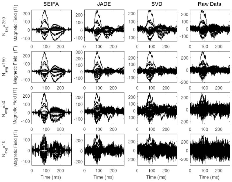
Denoising auditory-evoked responses. Each row shows the averaged auditory-evoked response for N_avg = 10, 50, 150, 250 respectively. Columns show the performance of SEIFA, JADE, SVD and Raw Data. Using SEIFA it can be seen that an evoked-response is observable even for averages with very small number of trials.

Figure 7.

Denoising performance for auditory-evoked data. The output SNIR is plotted as a function of the number of trials used in the averages. The inset shows the signals used as a surrogate reference for ground-truth response. Superior performance of SEIFA can be observed for averages from a small number of trials.

For real data the time courses at the sensors generated solely by the evoked sources, $y_{\mathit{\text{in}}}^{\ast }$, are not known, hence the previously defined denoising metric is not directly applicable. In an attempt to quantify the performances of the different methods a filtered version of the raw data for N_avg = 250 is used in place of $y_{\mathit{\text{in}}}^{\ast }$. Filtering was done using a zero-phase band-pass filter with cutoff frequencies of 1 and 100 Hz. Figure 7 shows the output SNIR as a function of N_avg and in the inset shows the signals used for $y_{\mathit{\text{in}}}^{\ast }$. For this example the output SNIR for SEIFA is nearly flat for N_avg > 50. SEIFA also produces the best performance of the four methods for N_avg < 225. As can be seen, the SVD method outperforms the others as N_avg becomes large since SVD becomes an ideal method in this case, i.e., for large SIR.

6.2.2 Artifact rejection

Results for the second experiment are shown in Figures 8-9. The stimulus is a binaural presentation of a 400 ms duration, 1 kHz tone every 1 s. Data was collected for N_avg = 100 trials. The subject was also asked to blink both eyes every other tone presentation to ensure that, for the purpose of this experiment, the eyeblink artifacts occur synchronously with the stimulus. This unrealistic scenario is chosen for demonstrative purposes only. SVD and SEIFA are applied separately to the left-half and right-half sensors. In both cases SVD uses the two largest singular vectors and SEIFA assumes L = 2 since two evoked sources are expected, one due to the eyeblink and one due to the auditory stimulus. The eyeblink may be considered to be ’evoked’ for this data due to the experimental design. Figure 8a shows the original trial-averaged magnetic fields recorded at the sensors. Notice that the subject was anticipating the regularly-occurring tones. It is surmised that the subject started the eyeblink early so that her eyes were shut just as the tone occurred. The auditory response is competely obscured by the eyeblinks, which have a much larger magnitude. Figures 8b and 8c show the two results for SVD, one for each subset of sensors. The contour plots are shown for t = 150ms since this corresponds to the expected timing of one of the two largest auditory responses and since the eyeblink magnitude at this time is relatively small. The reconstruction using the left-half sensors shows a reponse in A1, as desired. The reconstruction using the right-half sensor, however, does not show a response in A1.

Figure 8.

Auditory-evoked responses contaminated by eye-blink artifacts. Each factor localization plot in this figure and all subsequent ones consists of five panels. First, localizations are overlaid on the subjects' MRI. Three orthogonal projections - coronal (top left), sagittal (top right) and axial (center left) MRI slices are shown.In each MR overlay, all voxels having 80% or more of the energy found in the maximum-energy voxel (the energy of each voxel is time-averaged over the entire post-stimulus period) are shown in white.The bottom row shows the time-course of the cleaned evoked factors after denoising are also displayed. A contour map (center right) that shows the polarity and magnitude of the sensor signals in sensor space is shown for a particular instant of time as indicated by the vertical dotted line in the bottom panel. A. The averaged auditory-evoked responses that is dominated by the eye-blink artifact. B. SVD results for sensors in the left hemisphere, using 2 largest singular vectors. C. SVD results for sensors in the right hemisphere, using 2 largest singular vectors.

Figure 9.

Localization of SEIFA estimated factors for eye-blink data. Legend for each sub-figure is similar to figure 7. A and B. SEIFA results for first and second factor from sensors in left hemisphere. C and D. SEIFA results for the first and second factor from sensors in the right hemisphere. In each hemisphere, a factor can be localized to the eye-blink and another to auditory cortex.

Figures 9a and 9c show the reconstructions of the first of the two factors using SEIFA for the left and right hemispheres, respectively. These are clearly due to the eyeblink artifact. Figures 9b and 9d show the second factors for both hemispheres, which both show activity in A1. Notice that the extracted auditory responses have a significantly smaller magnitude than the eyeblink. This demonstrates the ability of SEIFA to remove artifacts, although it should be mentioned that there are other approaches that could be used for this particular dataset. Namely, one could use SVD and remove the most energetic singular-value component, which is expected to be related to the eyeblink.

6.2.3 Separation of evoked sources I

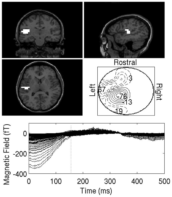
To highlight SEIFA's ability to separately localize evoked factors and sources, we conducted an experiment involving simultaneous presentation of auditory and somatosensory stimuli. We expected simultaneous activation of contralateral auditory and somatosensory cortex. A pure tone (400ms duration, 1kHz, 5 ms ramp up/down) was presented binaurally with a delay of 50 ms following a pneumatic tap on the left index finger. Averaging is performed over N_avg = 100 trials triggered on the onset of the tap. Results for this experiment are shown in Figure 10. Results are based on using the right hemisphere channels above contralateral somatosensory and auditory cortices. The figure shows localization and time-course of each of the three factors extracted by SEIFA. The first two factors localize to primary somatosensory cortex (SI), however with differential latencies. The first factor shows a peak response at a latency of 50 ms, whereas the second factor shows the response at a later latency. Interestingly, the third factor localizes to auditory cortex and the extracted time-course corresponds well to an auditory evoked response that is well-separated from the somatosensory response.

Figure 10.

Localization of SEIFA estimated evoked sources for auditory-somatosensory data in Experiment #3. Three factors extracted using SEIFA for the combined auditory/somato-sensory stimulus are shown. Legend for each sub-figure is identical to figure 7. A and B. Two factors that localize to somatosensory cortex correspond to and early and late somatosensory response. C. A third factor localizes to auditory cortex and has the time-course consistent with an auditory-evoked response.

6.2.4 Separation of evoked sources II

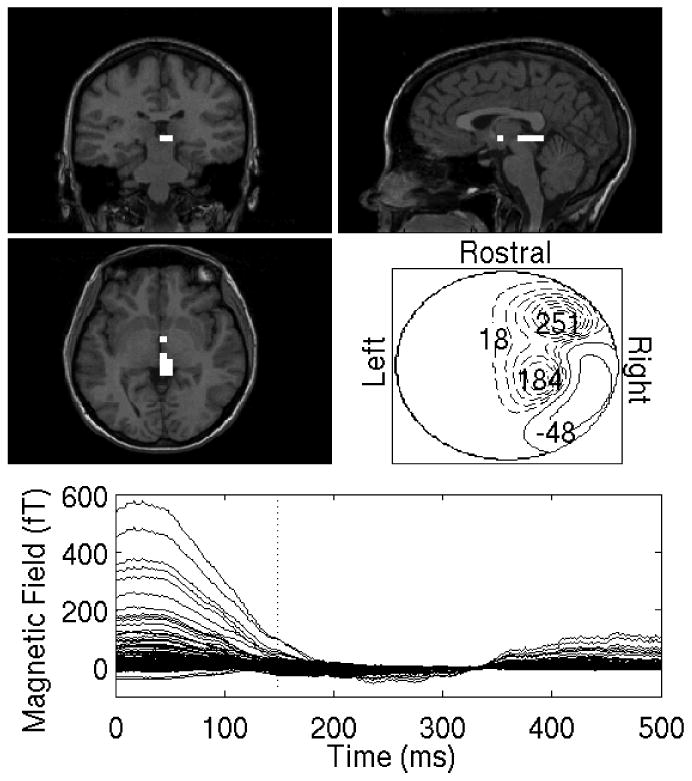
The patient involved in this example represents an interesting clinical case in that the auditory response in the right hemisphere is noticeably delayed relative to the response in the left hemisphere. This is particularly pronounced for the case of 500 Hz tones, such as used in this example. The cause of this anomaly is unknown but maybe be related to the presence of a brain tumor on one side. Auditory responses are otherwise normal. Responses to such data are normally analyzed by beamformer localization one hemisphere at a time. Beamforming of the entire sensor array produces (incorrect) localizations in the center of the brain due to the presence of highly correlated source activity in both hemispheres. SEIFA was run on data from the entire sensor array and results are shown in Figure 11. Figure 11a shows the SVD reconstruction, which is based on the two largest singular vectors. The reconstruction shows center of the head localization. This is expected since SVD is not able to separate spatially-distinct sources and the activation is symmetric with respect to the center of the head. SEIFA was able to successfully separate the sources in each hemisphere. Figures 11b-11c show the first and second factors extracted by SEIFA, respectively. The first factor shows significant activity near the left A1 and the second factor shows activity near the right A1. The time-course of these factors clearly shows the early response in the left hemisphere (∼85 ms) when compared with the right (∼100ms). Hence, SEIFA is able to separate constituent sources in this experiment.

Figure 11.

Localization of SEIFA estimated auditory-evoked sources in Patient F. Legend for each sub-figure same as in figure 7. A. SVD beamformer results using two largest singular vectors using sensors in both hemispheres localizes to the center of the head. B. Localization of the first factor esimated by SEIFA corresponds to auditory cortex in the left hemisphere and has an early response ( 85ms). C.Localization of the second factor estimated by SEIFA corresponds to auditory cortex in the right hemisphere with a later response ( 100ms)

7 Discussion

We have presented a novel algorithm for denoising, separation and localization of stimulus-evoked brain activity obtained from MEG and EEG measurements. Although, the results presented here focus on MEG data, the framework presented here is applicable to EEG data and combined measurements as well. We used a latent-variable probabilistic modeling approach to model sensor measurements as the sum of unobserved non-Gaussian stimulus-evoked sources, Gaussian interference sources and Gaussian sensor noise. We used a VB-EM algorithm to infer the latent variables and model parameters. We further exploited the pre-stimulus data to infer parameters of interference sources and sensor noise. We demonstrate the superior performance of our algorithm with other benchmarks both for simulations with high-noise and interference and small data lengths and with real data.

Whereas the framework presented in this paper bears some similarities to the independent components analysis (ICA) approach, there are several important differences. ICA algorithms learn unmixing matrices and are limited to square noiseless mixing of independent brain sources. In the case of measurement systems with 275 channels, for good performance dimensionality reduction is necessary. Often, SVD methods are used in conjunction with ICA algorithms for dimensionality reduction. Signal sub-space dimensionality estimation can be difficult for low SIR and SNR data and dimension reduction will result in erroneous results. In contrast, SEIFA learns unknown mixing matrices for cases that are not limited to square-mixing and offers a natural form of dimensionality reduction with no loss of information. Furthermore, it is optimal in non-zero noise and also can exploit pre-stimulus data to learn the interference model. As we have shown, SEIFA significantly outperforms JADE in our simulations, especially for short data lengths and high-noise conditions.

One advantage of the algorithm presented here is that it offers a principled way of model-order selection and to learn evoked source distributions. In our simulations and data analysis presented so far we have assumed that the number of factors L is known. In our algorithm, one can use the MAP estimates of the hyperparameters of the mixing matrices to estimate the number of factors by thresholding. Alternatively, one can determine the number of factors in the data by computing the evidence or marginal likelihood for different number of factors and then choose L such that the marginal likelihood of the data is maximized. This involves computing equation (46) for different model orders and choosing the model order that maximizes F. We also assume that the source distributions are known and correspond to damped and windowed sinusoids. Using the EM-algorithm, we can also in principle learn the means and variances of these mixture of Gaussian distribution parameters from the data. Such investigations of model-order selection and learning of source distributions within the SEIFA framework presented in this paper is currently under investigation.

SEIFA improves localization of denoised and separated sources with beamforming by computing regularized data covariance matrices of evoked sources and the noise. Localization of data denoised using SEIFA can be achieved by algorithms other than beamforming. Since SEIFA computes regularized evoked source and noise correlation matrices, it can also be used in conjunction with maximum-likelihood dipole estimation procedures and with MUSIC [24]. Such investigations are also currently underway.

Figure 1.

SEIFA Graphical Model. Left column shows the graphical model for pre-stimulus data. y is the observed spatiotemporal data, B is the interference factor loading matrix and u the unobserved interference factors. Right column shows the graphical model for post-stimulus data. Note the addition of stimulus-evoked factors x, which are modelled as a mixture of Gaussians defined by states s, and the stimulus-evoked factor loading matrix A. The dashed box encloses all the variables and the nodes outside the box indicate paramters, all of which are estimated from the data.

Appendix: The VB-EM Algorithm

This section outlines the derivation of the VB-EM algorithm that infers the SEIFA model from data.

7.1 Model

We start by rewriting the model in a form that explicitly includes the collective states s_n of the evoked factors as latent variables. Let r be a L-dimensional vector denoting a particular collective state: r = (r₁, r₂, …,r_L) denotes the configuration where evoked factor j is in state r_j = 1 : S_j; there are S = Π_j S_j configurations. Let the L-dimensional vector μ_r and diagonal L × L matrix ν_r denote the mean and precision, respectively, corresponding to collective state r, and let π_r denote its probability. Hence

$${\mu }_r=\left(\begin{array}{c}{\mu }_1,r_1\\ {\mu }_2,r_2\\ \cdots \\ {\mu }_L,r_L\end{array}\right),{\nu }_r=\left(\begin{array}{c}{\nu }_{1,r_1}\\ & {\nu }_{2,r_2}\\ & & \cdots & \\ & & & {\nu }_{L,r_L}\end{array}\right),{\pi }_r={\pi }_{1,r_1}{\pi }_{2,r_2}\cdots {\pi }_{L,r_L}$$ (38)

We now have

$$p(x_n|s_n=r)=\mathcal{N}(x_n|{\mu }_r,{\nu }_r),p(s_n=r)={\pi }_r$$ (39)

and from the i.i.d. assumption

$$\begin{array}{lll}p(x|s)\hfill & =\hfill & \prod _{n=N_0+1}^{N}p(x_n|s_n)\hfill \\ \hfill p(s)& =\hfill & \prod _{n=N_0+1}^N{\pi }_{s_n}\hfill \end{array}$$ (40)

The full joint distribution of the SEIFA model is given by

$$p(y,x,s,u,A,B)=p(y|x,u,A,B)p(x|s)p(s)p(u)p(A)p(B)$$ (41)

together with Eqs. (5,7,8,39,40).

7.2 Variational Bayesian Inference

The Bayesian approach, as discussed above, treats latent variables and parameters on equal footing: both are unobserved quantities for which posterior distributions must be computed. A direct application of Bayes' rule to the SEIFA model would compute the joint posterior over the latent variables x, s, u and parameters A, B

$$p(x,s,u,A,B|y)=\frac{1}{p(y)}p(y,x,s,u,A,B)$$ (42)

where the normalization constant p(y), termed the marginal likelihood, is obtained by integrating over all other variables

$$p(y)=\sum _s\int \mathit{\text{dx du dA dB}}p(y,x,s,u,A,B)$$ (43)

However, this exact posterior is computationally intractable, because the integral above cannot be obtained in closed form.

The VB approach approximates this posterior using a variational technique. The idea is to require the approximate posterior to have a particular factorized form, then optimize it by minimizing the Kullback-Leibler (KL) distance from the factorized form to the exact posterior. Here we choose a form which factorizes the latent variables from the parameters given the data,

$$p(x,s,u,A,B|y)\approx q(x,s,u,A,B|y)=q(x,s,u|y)q(A,B|y)$$ (44)

It is worth emphasizing that (1) beyond the factorization assumption, we make no further approximation when computing q, and (2) the factorized form still allows correlations among x, s, u, as well as among the matrix elements of A, B, conditioned on the data.

Rather than minimize the KL distance directly, it is convenient to start from an objective function defined by

$$\mathcal{F}[q]=\sum _s\int \mathit{\text{dx du dA dB}}q(x,s,u,A,B|y)[logp(y,x,s,u,A,B)-logq(x,s,u,A,B|y)]$$ (45)

It can be shown that

$$\mathcal{F}[q]=logp(y)-\mathit{\text{KL}}[q(x,s,u,A,B|y)||p(x,s,u,A,B|y)]$$ (46)

and since the marginal likelihood p(y) is independent of q, maximizing ( w.r.t. q is equivalent to minimizing the KL distance. Furthermore, ( is upper bounded by log p(y) because the KL distance is always nonnegative. Hence, any algorithm that successively maximizes ( , such as VB-EM, is guaranteed to converge.

7.3 Derivation of VB-EM

VB-EM is derived by alternately maximizing ( w.r.t. the two components of the posterior q. In the E-step one maximizes w.r.t. the posterior over latent variables q(x, s, u | y), keeping the second posterior fixed. In the M-step one maximizes w.r.t. the posterior over parameters q(A, B | y), keeping the first posterior fixed. When performing maximization, normalization of q must be enforced by adding two Lagrange multiplier terms to ( in (45).

Maximization is performed by setting the gradients to zero

$$\begin{array}{lll}\frac{\partial \mathcal{F}}{\partial q(x,s,u|y)}\hfill & =\hfill & {\langle logp(y,x,s,u,A,B)\rangle }_2-logq(x,s,u|y)+C_1=0\hfill \\ \frac{\partial \mathcal{F}}{\partial q(A,B|y)}\hfill & =\hfill & {\langle logp(y,x,s,u,A,B)\rangle }_1-logq(A,B|y)+C_2=0\hfill \end{array}$$ (47)

where C₁, C₂ are constants depending only on the data y and not on the variables that are used in the E- and M- steps. 〈·〉₁ denotes averaging only w.r.t. q(x, s, u | y), and 〈·〉₂ denotes averaging only w.r.t. q(A, B | y). Hence, the posteriors are given by

$$\begin{array}{lll}q(x,s,u|y)\hfill & =\hfill & \frac{1}{Z_1}exp[{\langle logp(y,x,s,u,A,B)\rangle }_2]\hfill \\ \hfill q(A,B|y)& =\hfill & \frac{1}{Z_2}exp[{\langle logp(y,x,s,u,A,B)\rangle }_1]\hfill \end{array}$$ (48)

where Z₁, Z₂ are normalization constants.

7.4 E-step

It follows from (48) that the posterior over u, x, s factorizes over time, and has different pre- and post-stimulus forms,

$$q(u,x,s|y)=\prod _{n=1}^{N_0}q(u_n|y_n)\cdot \prod _{n=N_0+1}^{N}q(u_n,x_n,s_n|y_n)$$ (49)

It also follows that in the pre-stimulus period q(u_n | y_n) is Gaussian in u_n, and in the post-stimulus period q(u_n, x_n, s_n | y_n) is Gaussian in u_n, x_n for a given s_n. To see this, consider log q(x, s, u | y) in (48) and observe that it is a sum over n, where the nth element depends only on x_n, u_n and the dependence is quadratic.

For the pre-stimulus period we obtain

$$q(u_n|y_n)=\mathcal{N}(u_n|{\overline{u}}_n,{\mathrm{\Phi }}^{-1})$$ (50)

with mean ū_n and covariance matrix Φ given by (10). (One first obtains Φ = (〈B^TλB〉 + I)⁻¹, and then performs the average using (61).) For the post-stimulus period, we write the posterior in the form

$$q(u_n,x_n,s_n|y_n)=q(x_n,u_n|s_n,y_n)q(s_n|y_n)$$ (51)

The first component on the right hand side is Gaussian

$$q(x_n,u_n|s_n=r,y_n)=q(x_n^{\prime }|s_n=r,y_n)=\mathcal{N}(x_n^{\prime }|{{\overline{x}}^{\prime }}_{\mathit{\text{rn}}},{\mathrm{\Gamma }}_r^{-1})$$ (52)

with mean ${{\overline{x}}^{\prime }}_{\mathit{\text{rn}}}$ and covariance matrix ${\mathrm{\Gamma }}_r^{-1}$ given by (12) (as for Φ above, one first obtains Γ_r = (〈A′^TλA′〉 + I)⁻¹, then applies (61).) ${{\mu }^{\prime }}_r$ and ${{\nu }^{\prime }}_r$ are defined as the L′ × 1 mean vector and L′ × L′ diagonal precision matrix, respectively, for collective state r, obtained from μ_r and ν_r of (38) by padding with M zeros

$${{\mu }^{\prime }}_r=\left(\begin{array}{c}{\mu }_r\\ 0_M\end{array}\right){{\nu }^{\prime }}_r=\left(\begin{array}{cc}{\nu }_r& \\ & 0_M\end{array}\right)$$ (53)

The state posterior is given by q(s_n = r | y_n) = π̄_rn (15), which is obtained by some further algebra.

It is useful to make explicit the correlations among the factors implied by their posteriors (50,52). For the pre-stimulus period we obtain

$$\langle u_n{u}_n^T\rangle ={\overline{u}}_n{\overline{u}}_n^T+\mathrm{\Phi }$$ (54)

For the post-stimulus period we obtain, conditioning on the collective state, $\langle x_n^{\prime }|s_n=r\rangle ={{\overline{x}}^{\prime }}_{\mathit{\text{rn}}}$ and $\langle x_n^{\prime }{x^{\prime }}_n^T|s_n=r\rangle ={{\overline{x}}^{\prime }}_{\mathit{\text{rn}}}{{\overline{x}}^{\prime }}_{\mathit{\text{rn}}}^T+{\mathrm{\Gamma }}_r$. In terms of x_n, u_n

$$\begin{array}{lll}\hfill \langle x_n|s_n=r\rangle & =\hfill & {\overline{x}}_{\mathit{\text{rn}}}\hfill \\ \hfill \langle u_n|s_n=r\rangle & =\hfill & {\overline{u}}_{\mathit{\text{rn}}}\hfill \\ \hfill \langle x_n{x}_n^T|s_n=r\rangle & =\hfill & {\overline{x}}_{\mathit{\text{rn}}}{\overline{x}}_{\mathit{\text{rn}}}^T+{\mathrm{\Gamma }}_{\mathit{\text{xx}}}^x\hfill \\ \hfill \langle u_n{u}_n^T|s_n=r\rangle & =\hfill & {\overline{u}}_{\mathit{\text{rn}}}{\overline{u}}_{\mathit{\text{rn}}}^T+{\mathrm{\Gamma }}_{\mathit{\text{uu}}}^r\hfill \\ \hfill \langle x_n{u}_n^T|s_n=r\rangle & =\hfill & {\overline{x}}_{\mathit{\text{rn}}}{\overline{u}}_{\mathit{\text{rn}}}^T+{\mathrm{\Gamma }}_{\mathit{\text{xu}}}^r\hfill \end{array}$$ (55)

where we have used (13,14).

To obtain the posterior means and correlations (21,23) we must sum over the collective state, since

$$\begin{array}{lll}\hfill \langle x_n^{\prime }\rangle & =\hfill & \sum _r\int {\mathit{\text{dx}}}_n^{\prime }q(s_n=r)q(x_n^{\prime }|s_n=r)x_n^{\prime }=\sum _r{\overline{\pi }}_{\mathit{\text{rn}}}\langle x_n^{\prime }|s_n=r\rangle \hfill \\ \langle x_n^{\prime }{x}_n^{\prime T}\rangle \hfill & =\hfill & \sum _r\int {\mathit{\text{dx}}}_n^{\prime }q(s_n=r)q(x_n^{\prime }|s_n=r)x_n^{\prime }{x}_n^{\prime ;T}=\sum _r{\overline{\pi }}_{\mathit{\text{rn}}}\langle x_n^{\prime }{x}_n^{\prime T}|s_n=r\rangle \hfill \end{array}$$ (56)

Eqs. (55,56) lead to the results (21,23).

7.5 M-step

It follows from (48) that the parameter posterior factorizes over the rows of the mixing matrices, and correlates their columns. Let wⁱ denote a column vector containing the ith row of the combined mixing matrix A′ = (A, B)

$$A^{\prime }=\left(\begin{array}{lll}\cdots \hfill & w^1\hfill & \cdots \hfill \\ \cdots \hfill & w^2\hfill & \cdots \hfill \\ \cdots \hfill & \cdots \hfill & \cdots \hfill \\ \cdots \hfill & w^K\hfill & \cdots \hfill \end{array}\right)$$ (57)

so $w_j^i=A_{\mathit{\text{ij}}}^{\prime }$. Then the posterior over each row is Gaussian

$$q(A,B|y)=q(A^{\prime }|y)=\prod _{i=1}^K\mathcal{N}(w^i|{\overline{w}}^i,{\mathrm{\lambda }}_i{\mathrm{\Psi }}^{-1})$$ (58)

with mean ${\overline{w}}_j^i={\overline{A}}_{\mathit{\text{ij}}}$ computed by (16). The precision matrix λ_iΨ⁻¹ is computed using (17). To see this, consider log q(A, B | y) in (48) and observe that it is a sum over i, where the ith element depends only on the ith rows of A, B and the dependence is quadratic.

It is now evident that p(A, B) of Eq. (9) is indeed a conjugate prior. Rewriting it in the form

$$p(A,B)=p(A^{\prime })=\prod _{i=1}^K\mathcal{N}(w^i|0,{\mathrm{\lambda }}_i{\alpha }^{\prime })$$ (59)

where α′ is a diagonal matrix with the hyperparameter matrices α, β on its diagonal, shows that its functional form is identical to that of the posterior (58), with Ψ⁻¹ replacing α′.

It is useful to make explicit the correlations among the elements of the mixing matrices implied by their posterior (58). They are $\langle A_{\mathit{\text{ij}}}^{\prime }{A}_{\mathit{\text{kl}}}^{\prime }\rangle ={\overline{A}}_{\mathit{\text{ij}}}^{\prime }{\overline{A}}_{\mathit{\text{kl}}}^{\prime }+{\delta }_{\mathit{\text{ik}}}{\mathrm{\Psi }}_{\mathit{\text{jl}}}/{\mathrm{\lambda }}_i$, or in terms of A, B

$$\begin{array}{lll}\langle A_{\mathit{\text{ij}}}{A}_{\mathit{\text{kl}}}\rangle \hfill & =\hfill & {\overline{A}}_{\mathit{\text{ij}}}{\overline{A}}_{\mathit{\text{kl}}}+{\delta }_{\mathit{\text{ik}}}\frac{1}{{\mathrm{\lambda }}_i}{({\mathrm{\Psi }}_{\mathit{\text{AA}}})}_{\mathit{\text{jl}}}\hfill \\ \langle B_{\mathit{\text{ij}}}{B}_{\mathit{\text{kl}}}\rangle \hfill & =\hfill & {\overline{B}}_{\mathit{\text{ij}}}{\overline{B}}_{\mathit{\text{kl}}}+{\delta }_{\mathit{\text{ik}}}\frac{1}{{\mathrm{\lambda }}_i}{({\mathrm{\Psi }}_{\mathit{\text{BB}}})}_{\mathit{\text{jl}}}\hfill \\ \langle A_{\mathit{\text{ij}}}{B}_{\mathit{\text{kl}}}\rangle \hfill & =\hfill & {\overline{A}}_{\mathit{\text{ij}}}{\overline{B}}_{\mathit{\text{kl}}}+{\delta }_{\mathit{\text{ik}}}\frac{1}{{\mathrm{\lambda }}_i}{({\mathrm{\Psi }}_{\mathit{\text{AB}}})}_{\mathit{\text{jl}}}\hfill \end{array}$$ (60)

where we used (18). It follows that

$$\begin{array}{lll}\hfill \langle A^T\mathrm{\lambda }A\rangle & =\hfill & {\overline{A}}^T\mathrm{\lambda }\overline{A}+K{\mathrm{\Psi }}_{\mathit{\text{AA}}}\hfill \\ \hfill \langle B^T\mathrm{\lambda }B\rangle & =\hfill & {\overline{B}}^T\mathrm{\lambda }\overline{B}+K{\mathrm{\Psi }}_{\mathit{\text{BB}}}\hfill \\ \hfill \langle {A^{\prime }}^T\mathrm{\lambda }{A}^{\prime }\rangle & =\hfill & {{\overline{A}}^{\prime }}^T\mathrm{\lambda }{\overline{A}}^{\prime }+K\mathrm{\Psi }\hfill \end{array}$$ (61)

which are needed for (10,12).

To obtain the update rules for the hyperparameters (19), observe that the part of the objective function ( (45) that depends on α, β is

$$\langle logp(A)+logp(B)\rangle$$ (62)

where the averaging is w.r.t. the posterior q. Next, compute the derivative of this expression w.r.t. α, β and set it to zero. The solution of the resulting equation is (19). It is easier to first compute the derivative and then apply the average. Similarly, to obtain the update rule for the noise precision (20), observe that the part of that depends on λ is

$$\langle logp(y|x,u,A,B)+logp(A)+logp(B)\rangle$$ (63)

and set its derivative w.r.t. λ to zero.

References

- 1.Attias H. Independent factor analysis. Neural Comput. 1999;11(4):803–51. doi: 10.1162/089976699300016458. [DOI] [PubMed] [Google Scholar]
- 2.Baillet S, Mosher JC, Leahy RM. Electromagnetic brain mapping. Signal Processing Magazine. 2001;18:14–30. [Google Scholar]
- 3.Baryshnikov BV, Van Veen BD, Wakai RT. Maximum-likelihood estimation of low-rank signals for multiepoch MEG/EEG analysis. IEEE Trans Biomed Eng. 2004;51(11):1981–93. doi: 10.1109/TBME.2004.834285. [DOI] [PubMed] [Google Scholar]
- 4.Bell Antony J, Sejnowski Terrence J. An information maximisation approach to blind separation and blind deconvolution. Neural Computation. 1995;7(6):1129–1159. doi: 10.1162/neco.1995.7.6.1129. [DOI] [PubMed] [Google Scholar]
- 5.Berg P, Scherg M. Dipole modelling of eye activity and its application to the removal of eye artefacts from the EEG and MEG. Clin Phys Physiol Meas. 1991;12(Suppl A):49–54. doi: 10.1088/0143-0815/12/a/010. [DOI] [PubMed] [Google Scholar]
- 6.Bijma F, de Munck JC, Bocker KB, Huizenga HM, Heethaar RM. The coupled dipole model: an integrated model for multiple MEG/EEG data sets. Neuroimage. 2004;23(3):890–904. doi: 10.1016/j.neuroimage.2004.06.038. [DOI] [PubMed] [Google Scholar]
- 7.Bijma F, de Munck JC, Huizenga HM, Heethaar RM. A mathematical approach to the temporal stationarity of background noise in MEG/EEG measurements. Neuroimage. 2003;20(1):233–43. doi: 10.1016/s1053-8119(03)00215-5. [DOI] [PubMed] [Google Scholar]
- 8.Cardoso Jean-François. High-order contrasts for independent component analysis. Neural Computation. 1999 Jan;11(1):157–192. doi: 10.1162/089976699300016863. [DOI] [PubMed] [Google Scholar]
- 9.de Munck JC, Bijma F, Gaura P, Sieluzycki CA, Branco MI, Heethaar RM. A maximum-likelihood estimator for trial-to-trial variations in noisy MEG/EEG data sets. IEEE Trans Biomed Eng. 2004;51(12):2123–8. doi: 10.1109/TBME.2004.836515. [DOI] [PubMed] [Google Scholar]
- 10.de Weerd JP. Facts and fancies about a posteriori wiener filtering. IEEE Trans Biomed Eng. 1981;28(3):252–7. doi: 10.1109/TBME.1981.324697. [DOI] [PubMed] [Google Scholar]
- 11.de Weerd JP. A posteriori time-varying filtering of averaged evoked potentials. i. introduction and conceptual basis. Biol Cybern. 1981;41(3):211–22. doi: 10.1007/BF00340322. [DOI] [PubMed] [Google Scholar]
- 12.de Weerd JP, Kap JI. A posteriori time-varying filtering of averaged evoked potentials. ii. mathematical and computational aspects. Biol Cybern. 1981;41(3):223–34. doi: 10.1007/BF00340323. [DOI] [PubMed] [Google Scholar]
- 13.Ebersole JS. Magnetoencephalography/magnetic source imaging in the assessment of patients with epilepsy. Epilepsia. 1997;38(Suppl 4):S1–5. doi: 10.1111/j.1528-1157.1997.tb04533.x. [DOI] [PubMed] [Google Scholar]
- 14.Hmlinen M, Hari R, Ilmoniemi RJ, Knuutila J, Lounasmaa OV. Magnetoencephalography – theory, instrumentation, and applications to noninvasive studies of the working human brain. Reviews of Modern Physics. 1993;65:413–497. [Google Scholar]
- 15.Ikeda S, Toyama K. Independent component analysis for noisy data–MEG data analysis. Neural Netw. 2000;13(10):1063–74. doi: 10.1016/s0893-6080(00)00071-x. [DOI] [PubMed] [Google Scholar]
- 16.James Christopher J, Gibson Oliver J. Temporally constrained ICA: an application to artifact rejection in electromagnetic brain signal analysis. IEEE Trans Biomed Eng. 2003;50:1108–1116. doi: 10.1109/TBME.2003.816076. [DOI] [PubMed] [Google Scholar]
- 17.Jordan MI, editor. Learning in Graphical Models. The MIT Press; Cambridge, Massachusetts: 1998. [Google Scholar]
- 18.Joyce Carrie A, Gorodnitsky Irina F, Kutas Marta. Automatic removal of eye movement and blink artifacts from EEG data using blind component separation. Psychophysiology. 2004;41:313–325. doi: 10.1111/j.1469-8986.2003.00141.x. [DOI] [PubMed] [Google Scholar]
- 19.Jung TP, Makeig S, Humphries C, Lee TW, McKeown MJ, Iragui V, Sejnowski TJ. Removing electroencephalographic artifacts by blind source separation. Psychophysiology. 2000;37(2):163–78. [PubMed] [Google Scholar]
- 20.Lee PL, Wu YT, Chen LF, Chen YS, Cheng CM, Yeh TC, Ho LT, Chang MS, Hsieh JC. Ica-based spatiotemporal approach for single-trial analysis of postmovement MEG beta synchronization. Neuroimage. 2003;20(4):2010–30. doi: 10.1016/j.neuroimage.2003.07.024. [DOI] [PubMed] [Google Scholar]
- 21.Lutkenhoner B, Wickesberg RE, Hoke M. A posteriori wiener filtering of evoked potentials: comparison of three empirical filter estimators. Rev Laryngol Otol Rhinol (Bord) 1984;105(2):153–6. [PubMed] [Google Scholar]
- 22.Makeig S. Response: event-related brain dynamics – unifying brain electrophysiology. Trends Neurosci. 2002;25(8):390. doi: 10.1016/s0166-2236(02)02198-7. [DOI] [PubMed] [Google Scholar]
- 23.Makeig S, Jung TP, Bell AJ, Ghahremani D, Sejnowski TJ. Blind separation of auditory event-related brain responses into independent components. Proc Natl Acad Sci U S A. 1997;94(20):10979–84. doi: 10.1073/pnas.94.20.10979. [DOI] [PMC free article] [PubMed] [Google Scholar]
- 24.Mosher JC, Lewis PS, Leahy RM. Multiple dipole modeling and localization from spatio-temporal MEG data. IEEE Trans Biomed Eng. 1992;39(6):541–57. doi: 10.1109/10.141192. [DOI] [PubMed] [Google Scholar]
- 25.Neal RM, Hinton G. A view of the EM algorithm that justifies incremental, sparse and other variants. In: Jordan MI, editor. Learning in Graphical Models. Kluwer Academic Publishers; Dordrecht: 1998. pp. 355–368. [Google Scholar]
- 26.Rubin DB, Thayer DT. EM algorithms for ML factor analysis. Psychometrika. 1982:69–76. [Google Scholar]
- 27.Sander Tilmann H, Wübbeler Gerd, Lueschow Andreas, Curio Gabriel, Trahms Lutz. Cardiac artifact subspace identification and elimination in cognitive MEG data using timedelayed decorrelation. IEEE Trans Biomed Eng. 2002;49:345–354. doi: 10.1109/10.991162. [DOI] [PubMed] [Google Scholar]
- 28.Sekihara K, Nagarajan SS, Poeppel D, Marantz A. Asymptotic snr of scalar and vector minimum-variance beamformers for neuromagnetic source reconstruction. IEEE Trans Biomed Eng. 2004;51(10):1726–34. doi: 10.1109/TBME.2004.827926. [DOI] [PMC free article] [PubMed] [Google Scholar]
- 29.Sekihara K, Nagarajan SS, Poeppel D, Marantz A, Miyashita Y. Reconstructing spatio-temporal activities of neural sources using an MEG vector beamformer technique. IEEE Trans Biomed Eng. 2001;48(7):760–71. doi: 10.1109/10.930901. [DOI] [PubMed] [Google Scholar]
- 30.Sekihara K, Nagarajan SS, Poeppel D, Marantz A, Miyashita Y. Application of an meg eigenspace beamformer to reconstructing spatio-temporal activities of neural sources. Human Brain Mapping. 2002;15:199–215. doi: 10.1002/hbm.10019. [DOI] [PMC free article] [PubMed] [Google Scholar]
- 31.Sekihara K, Sahani M, Nagarajan SS. Localization bias and spatial resolution of adaptive and non-adaptive spatial filters for MEG source reconstruction. Neuroimage. 2005;25(4):1056–1067. doi: 10.1016/j.neuroimage.2004.11.051. [DOI] [PMC free article] [PubMed] [Google Scholar]
- 32.Tang AC, Pearlmutter BA, Malaszenko NA, Phung DB, Reeb BC. Independent components of magnetoencephalography: localization. Neural Comput. 2002;14(8):1827–58. doi: 10.1162/089976602760128036. [DOI] [PubMed] [Google Scholar]
- 33.Van Veen BD, van Drongelen W, Yuchtman M, Suzuki A. Localization of brain electrical activity via linearly constrained minimum variance spatial filtering. IEEE Trans Biomed Eng. 1997;44(9):867–80. doi: 10.1109/10.623056. [DOI] [PubMed] [Google Scholar]
- 34.Vigario R, Sarela J, Jousmaki V, Hamalainen M, Oja E. Independent component approach to the analysis of EEG and MEG recordings. IEEE Trans Biomed Eng. 2000;47(5):589–93. doi: 10.1109/10.841330. [DOI] [PubMed] [Google Scholar]