

Abstract
Most statistical analyses of fMRI data assume that the nature, timing and duration of the psychological processes being studied are known. However, in many areas of psychological inquiry, it is hard to specify this information a priori. Examples include studies of drug uptake, emotional states or experiments with a sustained stimulus. In this paper we assume that the timing of a subject's activation onset and duration are random variables drawn from unknown population distributions. We propose a technique for estimating these distributions assuming no functional form, and allowing for the possibility that some subjects may show no response. We illustrate how these distributions can be used to approximate the probability that a voxel/region is activated as a function of time. Further a procedure is discussed that uses a hidden Markov random field model to cluster voxels based on characteristics of their onset, duration, and anatomical location. These methods are applied to an fMRI study (n = 24) of state anxiety, and are well suited for investigating individual differences in state-related changes in fMRI activity and other measures.
Keywords: fMRI, change-point, density estimation, hidden Markov random field model, state-related changes, statistical analysis
1 Introduction
The voxel-wise general linear model (GLM) (Worsley and Friston, 1995) has arguably become the dominant approach towards analyzing fMRI data. It tests whether variability in a voxel's time course can be explained by a set of a priori defined regressors that model predicted responses to psychological events of interest. The GLM has been shown to be a powerful and efficient way of analyzing data as long as the nature, timing and duration of the psychological processes under study can be specified in advance (Loh, Lindquist, and Wager, 2008). However, in many areas of psychological inquiry, it is hard to specify this information a priori. Examples include studies of drug uptake, emotional states or experiments with sustained stimulus. In these situations standard GLM-based analysis may not be able to accurately model brain activity and new kinds of statistical models are needed to capture state-related changes in activity.
The effectiveness of the GLM in modeling state-related activity is limited in several ways. One limitation concerns the match between the desired inference and that supported by the model. In many experiments, the primary parameter of interest may be the timing of activation rather than the magnitude. However, a GLM analysis does not allow for direct inference on the onset and duration of activation. The interpretable parameters of the GLM model refer to the magnitude rather than the timing of the activation response. A set of regressors which do a poor job of modeling the true activation profile will have smaller estimated magnitudes than a set which accurately reflects the timing, but there is no way to directly estimate the true timing of activation. It may be possible to indirectly account for timing differences by using a set of flexible basis functions in the GLM (Friston, Fletcher, Josephs, Holmes, Rugg, and Turner, 1998; Glover, 1999). However, the a priori specification of an onset time is still necessary for the definition of the regressors, and they are typically only able to account for very small timing shifts. Further, such models are usually constrained in their flexibility in order to avoid substantial losses in power and stability (Calhoun, Stevens, Pearlson, and Kiehl, 2004; Lindquist and Wager, 2007; Lindquist, Loh, Atlas, and Wager, 2008). Another limitation of the GLM approach is related to reproducibility. Suppose that a brain region reproducibly responds to a particular emotion, though the onset and duration varies across participants and studies depending on the particular task demands and individual propensities. In this case, there is no GLM model that will give reproducible activation in the region of interest. However, a more flexible model may capture consistencies in activation magnitude while allowing for variations in timing.
For the situations outlined above, model flexibility is critical. Models that permit more data-driven estimates of activation, and inferences on when and for how long activation occur, may be advantageous for discovering state-related activations whose timing can only be specified loosely a priori. Rather than treating psychological activity as a zero-error fixed effect specified by the analyst (as in the GLM) and testing for brain changes that fit the specified model, data-driven approaches attempt to characterize reliable patterns in the data, and relate those patterns to psychological activity post hoc. One particularly popular approach is independent components analysis (ICA) (Calhoun, Adali, Pearlson, and Pekar, 2001; McKeown and Makeig, 1998; Beckmann and Smith, 2004). Though ICA has proven efficient in identifying brain activity patterns (components) that are reliable across participants and state-related changes in activity that can subsequently be related to psychological processes, they do not provide statistics for inferences about whether a component varies over time and when changes occur in the time series; subsequent GLM-based tests have been used for this purpose. In addition, because they do not contain any model information, they capture regularities whatever the source; thus, they are highly susceptible to noise, and components can be dominated by artifacts.
In sum, the GLM approach is attractive due to its power to test statistical hypotheses, while data-driven techniques are attractive due to their flexibility to handle uncertainties in the timing of activation. For these reasons, there is interest in extending the GLM framework to enable it to handle uncertainties in onset and duration. In past work (Lindquist, Waugh, and Wager, 2007; Lindquist and Wager, 2008), we have introduced a technique that allows the predicted signal to depend non-linearly on the transition time. It is a multi-subject extension of the exponentially weighted moving average (EWMA) method used in change-point analysis. We extended existing EWMA models for individual subjects so that they were applicable to fMRI data, and developed a group analysis using a hierarchical model, which we termed Hierarchical EWMA (HEWMA). The HEWMA method can be used to analyze fMRI data voxel-wise throughout the brain, data from regions of interest, or temporal components extracted using ICA or similar methods. While the HEWMA method is exploratory in nature, it retains the inferential nature of the GLM approach. Further, the HEWMA framework includes a step for estimating the time when the activation profile in the population changes from a baseline state to a state of activation, which we refer to as the “change point”, in keeping with statistical literature on similar models.
A drawback of this estimation procedure is that the change points were assumed to be fixed across subjects, i.e. all subjects change states (e.g., from inactive to activated) at the same time. In this work, we relax this condition, assuming that the change points for each subject are randomly drawn from unknown population distributions (see Figure 1). We develop a procedure for estimating, for each individual voxel, the distributions of onset and duration of the BOLD response. We estimate these distributions assuming no functional form, and allowing for the possibility that some subjects may show no response at all. In our model we allow for up to two change points in each subject's voxel time course, signifying the beginning and end of the activated state. Joseph and Wolfson (Joseph and Wolfson, 1993) addressed the problem of maximum likelihood estimation in multi-path change-point problems. The procedure described in this paper is an extension of their method applied to multi-subject fMRI data with multiple change points. We further illustrate how these distributions can be used to approximate the probability that a voxel is active at a given time point.
Figure 1.
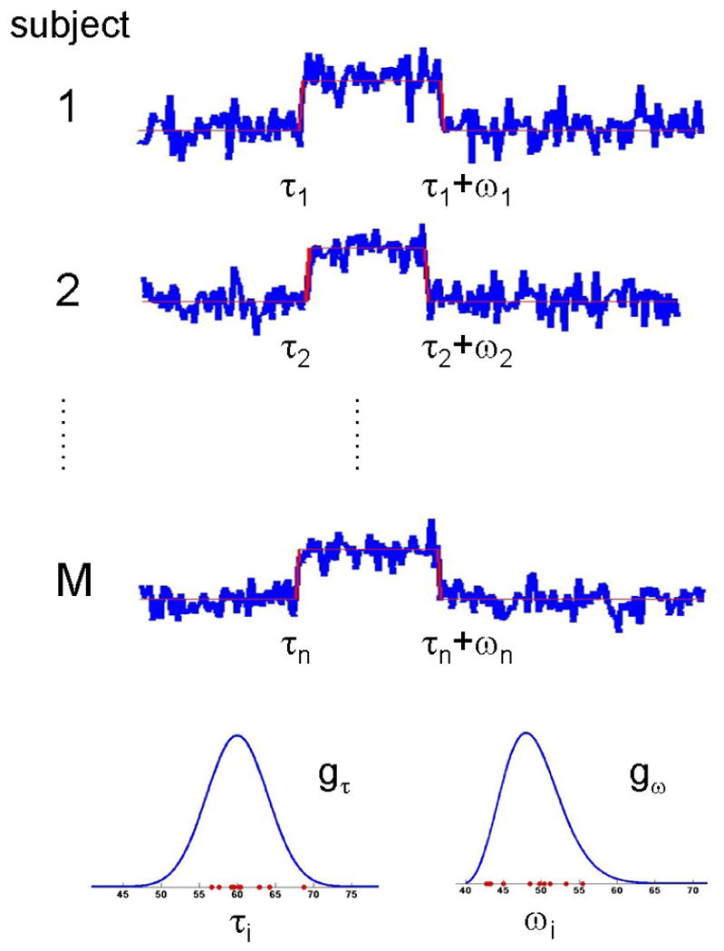
In our model formulation each subject is allowed to switch states up to two times. The timing of these state-changes are determined by change points τi and ωi, chosen at random from the population distributions gτ and gω, respectively. In this formulation, gτ represents the population distribution of the onset of activation, while gω represents the population distribution of the duration.
This model is formulated for a state-related shift from a baseline to activated state and a subsequent return to baseline at a later, unknown time. This type of model is suited for studying state-related, single epoch paradigms, such as acute social stress (Wager, Waugh, Lindquist, Noll, Fredrickson, and Taylor, 2009b; Wager, van Ast, Hughes, Davidson, Lindquist, and Ochsner, 2009a), bolus drug infusion (Wise, Williams, and Tracey, 2004; Breiter, Gollub, Weisskoff, Kennedy, Makris, Berke, Goodman, Kantor, Gastfriend, Riorden, Mathew, Rosen, and Hyman, 1997), or social exclusion (Eisenberger, Lieberman, and Williams, 2003). In each of these paradigms, scanning begins during a baseline condition, and partway into scanning, an irreversible event happens (stressor, exclusion, drug delivery), which persists for a period of time. The condition is either reversed with a new manipulation (stress-relieving instructions, inclusion) or the brain returns to baseline naturally after some period of time (e.g., drug washout). These situations are less readily amenable to GLM-based analyses, making change-point models an appealing choice for analysis.
Once the activation onset and duration have been estimated for individual voxels, it is important to identify patterns of similar activation across voxels and across brain regions. As a final step of our analysis, we perform spatial clustering of voxels according to onset and duration values and anatomical location using a hidden Markov random field model. These types of models have been successfully used to segment images based on structural characteristics (Zhang, Brady, and Smith, 2001; Zhang, Johnson, Little, and Cao, 2008). Here we use a multivariate hidden Markov random field (HMRF) model to estimate the grouping of voxels based on their activation characteristics.
In summary, in this work we develop an approach towards estimating voxel-specific distributions of onset times and durations from the fMRI response, by modeling each subject's onset and duration as random variables drawn from an unknown population distribution. We also discuss a technique for performing spatial clustering of voxels according to onset and duration characteristics, and anatomical location using an HMRF model. Together these procedures provide a spatio-temporal model for dealing with data with uncertain onset and duration.
2 Theory
In this section we develop the ideas surrounding the estimation of population distributions for onset and duration of activation and for performing spatial clustering using the HMRF approach.
2.1 Multi-subject change point modeling
We model each voxels time course using a two-state model where at a given point in time a subject is considered to be either in an active or an inactive state. For each voxel, suppose we have data from M subjects measured at N different time points. For subject i, the time profile of the voxel is modeled as a sequence of independent identically distributed random observations yij, j = 1 … N, which may at an unknown time point τi undergo a shift in mean of unknown magnitude. This shift, referred to as a change point, represents the location where the time course shifts from the inactive to the active state. Further, this shift may be followed by a return to the inactive state at time τi + ωi, where the second change point ωi is also unknown. In this formulation τi represents the onset of activation for subject i, while ωi represents the duration. Both τi and ωi are assumed to be randomly drawn from separate unknown population distributions denoted gτ and gω, respectively. Fig. 1 provides an illustration.
The time course for each voxel can be modeled as arising from a mixture of two distributions, one corresponding to the active and the other to the inactive state, with the added constraint that, except where separated by a change point, temporally contiguous observations come from the same mixture component. If f1 is the density of observations generated during the non-activated state, and f2 is the density for the activated state, the positions of the change points, τi and τi + ωi, determine whether each observation yij was drawn from f1 or f2.
In this work, we assume that f1 and f2 are both Gaussian, and seek to estimate their parameters θ1 = (μ1, , i = 1 … M) and θ2 = (μ2, , i = 1, … M), as well as the population distributions for the change points τi and ωi. While the change points are allowed to vary across subjects, the means of the baseline and activation states, μ1 and μ2, are assumed to be equal for all subjects. In addition, the variances are assumed to be constant across time, but allowed to differ across subjects. In order to fit the model, τ = {τi}i=1…M and ω = {ωi}i=1…M are treated as missing data. The sequences of onset times {τi} and durations {ωi} are both assumed to be independent and identically distributed sets of discrete random variables. No functional form is assumed for the population distributions gτ(t) = P(τi = t) and gω(k) = P(ωi = k). Rather, gω(k) is estimated for the time points k = ωmin, …, ωmax and gτ(t) is estimated for t = 1, …, N −ωmin, where ωmin and ωmax are specified by the researcher. Note that the values of ωmin and ωmax could be set to 1 and N, respectively, but for speed of estimation we typically choose a smaller range of reasonable values for activation duration. Finally, the onsets and durations are assumed to be independent of one another.
Given the onset and duration of the signal and assuming independence in time, the joint density of the time series for subject i is the product of the densities of the yij, i.e.
| (1) |
Since in practice τ and ω are unknown, the data can be modeled by a mixture of components with different values of τ and ω weighted by gτ(·) and gω(·), making the joint likelihood given the entire data Y = {yij}, i = 1 … M, j = 1 … N,
| (2) |
To estimate the unknown parameters θ = {μ1, μ2, , gτ(·), gω(·)} we must compute
| (3) |
The maximum likelihood estimates (MLEs) can not be computed directly from the likelihood function, but by treating τi and ωi as missing data, we can employ the EM-algorithm (Dempster, Laird, and Rubin, 1977) to compute the estimates. The details of the EM-algorithm implementation are in Appendix A. Here we simply note that as the EM-algorithm is deterministic, it can converge to a local maximum and is sensitive to initial parameter estimates. The analysis should therefore be repeated under various initial conditions until the investigator is reasonably certain that the global MLE has been found.
2.1.1 Estimating gτ and gω with smoothness constraints
The voxel-specific estimates of gτ and gω can be defined as the MLEs under the change-point mixture model formulated above. The drawback of this approach is that gτ(τ) is assumed to be independent of its neighboring terms gτ(τ − 1) and gτ (τ + 1) for each possible value of τ, resulting in estimated densities which tend to be noisy and rough (see Fig. 2 for an example). It is common in non-parametric density estimation to perform some regularization of the estimated density, based on the assumption that in most situations, g(τ) will tend to be close to g(τ + 1), meaning that even if g does not assume a standard parametric form (e.g., Gaussian), we still assume it will be relatively smooth. As regularization reduces the variability in the density estimates, it is often considered to be preferable to unregularized non-parametric MLE. To obtain smoother estimates, we can incorporate additional smoothness assumptions about gτ and gω into the model formulation. We first discuss two equivalent approaches: maximum penalized likelihood and a Bayesian approach that allows for the inclusion of a prior on gτ and/or gω. In addition, we also discuss the smoothed EM-algorithm (Silverman, Jones, Wilson, and Nychka, 1990).
Figure 2.
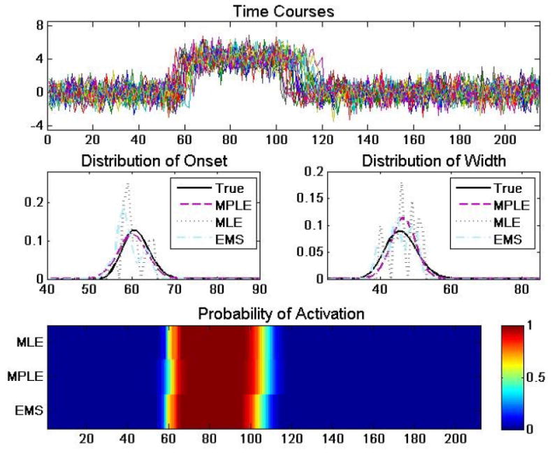
(A) An example of 20 simulated time courses of length 215 whose onset and duration were randomly sampled from population distributions gτ and gω, respectively. (B) The true distribution of gτ (bold black) compared to estimates obtained using the MLE, MPLE and EMS approaches. Note the roughness of the estimate obtained using the MLE approach. (C) The same results for gω. (D) A heat map depicting the probability of activation as a function of time computed using the MLE, MPLE and EMS estimates of gτ and gω.
Maximum penalized likelihood estimation (MPLE) (Silverman, 1986) imposes a penalty term on the log-likelihood function, creating a new objective function from which the parameters are estimated:
| (4) |
where l(·) is the likelihood function defined in (2), J is a penalty function and λ is a tuning parameter controlling the relative impact of the penalty term. The use of the penalized likelihood necessitates the specification of the tuning parameter λ, which can either be pre-specified or incorporated directly into the estimation procedure. The penalty term can alternatively be interpreted as the logarithm of the prior density in a Bayesian formulation. If we incorporate priors on gτ and gω into the model, the log posterior distribution will contain a term which behaves like a penalty term with respect to the maximum a posteriori (MAP) estimates of gτ and gω. The standard maximum likelihood estimates for gτ and gω can in this context be viewed as being the MAP estimates calculated using a non-informative prior.
We have found that rather than placing priors directly on gτ and gω, it is beneficial to first model them as functions constrained to be non-negative and sum to 1, thus ensuring that they are proper density functions, and thereafter place priors on the parameters of these functions. We begin by defining two auxiliary variables ητ and ηk and modeling gτ and gω using the softmax function (Bishop, 2006), i.e.
| (5) |
and
| (6) |
Next, we assume that ητ ∼ N(0, Στ) and ηω ∼ N(0, Σω). To obtain a smooth solution we define both covariance terms to be on the form
| (7) |
where h represents the precision of the covariance and k allows one to truncate the co-variance after a certain number of observations. In general, our prior/penalty imposes a covariance structure on the density across values of τ and ω in which nearby values have positive covariance, which decreases exponentially as a function of proximity. The parameters h and k impact the width and smoothness, respectively, of the estimated distributions. Larger values of h result in very peaked distributions (potentially with peaks at multiple modes), smaller values give wider distributions. Small values of k allow for more jagged distributions, while still shrinking the estimates at most possible values of τ and ω. Values of h and k can either be determined empirically, or in a more principled manner using leave-one-out cross-validation. We take the former approach in the first simulation study, while we take the latter approach in the second simulation study and in the analysis of experimental data. Cross-validation is performed by finding the values of h and k that minimize the average mean squared error between the left-out time course and expected time course obtained from fitting the model to the remaining M − 1 subjects. To fit the maximum penalized likelihood model one needs to use a generalized EM-algorithm outlined in Appendix B.
The smoothed EM-algorithm (Silverman, Jones, Wilson, and Nychka, 1990) is an alternative approach that adds a smoothing step to each iteration of the standard EM-algorithm. For our problem, after the model parameters are estimated using maximum likelihood in the M-step, a pre-defined smoothing kernel can be applied to the estimates of gτ and gω, and these smoothed estimates are used in the next iteration. We use a simple local smoother,
| (8) |
to create a smoothed version of , the estimated density from the kth iteration of the EM-algorithm. We then pass on to the (k + 1)th iteration in place of .
In certain special cases the smoothed EM can be shown to be related to the maximum penalized likelihood estimates, but is essentially an ad hoc procedure without rigorous theoretical justification. Fig. 2 compares the results of the standard MLE, MPLE, and smoothed EM estimation procedures on simulated data.
2.2 Spatial Clustering
A natural unit of analysis in fMRI is a multi-voxel region whose voxels show similar properties with respect to the timing of activation and de-activation. We wish to create a segmented image consisting of cluster labels for each voxel in the brain, identifying which voxels exhibit similar behavior with respect to onset and duration of activation. We expect the clusters containing similar voxels will exhibit some spatial coherence, but allow clusters which consist of networks of spatially disjoint regions. To achieve these goals we implement a hidden Markov random field model described below. We begin by giving a brief overview of Markov random field models.
2.2.1 Markov random field models
We use a Markov random field (MRF) model for the unobserved field of cluster labels to describe the spatial structure of the image. MRFs are a way to incorporate an assumption of spatial smoothness into the image segmentation algorithm. In our application we assume that two neighboring voxels are somewhat more likely to be in the same cluster than two non-neighboring voxels. The global dependence properties of a MRF are controlled by the specification of local properties, i.e. the spatial dependence structure of the entire image is determined completely by the conditional distribution of a voxel given neighboring voxels. This property eases the computational burden and is a reasonable assumption in many applications. The use of MRFs in image analysis was popularized by, among others, Besag (Besag, 1974) and Geman and Geman (Geman and Geman, 1984).
Let S = (1, 2, …, N) be the index of voxels in the image. Suppose each voxel has a label from the set
 = {1, 2, …, L} where L denotes the total number of clusters. Further let X = (x1, x2, …, xN), be the configuration of labeled voxels, where xi ∈
for every i ∈ S. The collection of all possible configurations of labeled sites, denoted
= {1, 2, …, L} where L denotes the total number of clusters. Further let X = (x1, x2, …, xN), be the configuration of labeled voxels, where xi ∈
for every i ∈ S. The collection of all possible configurations of labeled sites, denoted
 , is then
| (9) |
A random field X is said to be a Markov Random Field if after conditioning on the cluster labels of its neighborhood, the probability that a given voxel belongs to any particular cluster is independent of the rest of the image. The neighborhoods are defined by a neighborhood system, which in our application consists of the 4 immediately adjacent voxels.
An important theoretical result in Markov random field theory is that any MRF can be equivalently characterized by a Gibbs distribution on X = (x1, …, xN) of the form
| (10) |
where U(X) is called the energy function. In this application we consider models with only pair-wise interactions between voxels. Let i ∼ j denote that xi and xj are neighbors. We can then write the energy function as
| (11) |
the exact form of which will be described below.
2.2.2 Hidden Markov random field models
A Hidden Markov Random Field (HMRF) model derives from the concept of a Hidden Markov Model. In an HMRF model, the random field of cluster labels, X, is unobserved while the data D is observed on S. At each voxel, we assume that the observed value di, which may be multivariate, is drawn from a probability distribution whose parameters depend on the cluster to which it belongs. Given xi = l, the conditional distribution of di is
| (12) |
We assume that that the functional form of f(·) is the same for each l ∈
, and that the di are conditionally independent of one another given the field X, i.e.
| (13) |
The joint density of an (xi, di) pair given the neighborhood X i is given by
| (14) |
and thus the marginal distribution of di given the labels of neighboring sites is
| (15) |
If we assume that the random variables xi are independent of one another the HMRF reduces to a finite mixture model with mixing weights all equal to 1/L.
In our application, the observed data in the HMRF model consists of features estimated from the fMRI time courses such as the expected value and standard deviation of the onset and duration in the population, as well as the difference in means between states. Further, we assume that f(·) is multivariate Gaussian with dimension p, where p is the number of features; typically equal to five in our application. Finally, we also need to model the distribution of the unobserved cluster labels X. We choose a model of the form (10) with
| (16) |
where 1xi=xj is equal to 1 if xi and xj belong to the same cluster, and 0 otherwise. The local characteristics of this model are then given by
| (17) |
Here the β parameters control the amount of spatial coherence, with larger values giving increased coherence. If βij = β for all i and j, this is the Potts model, a well-studied model originating in statistical mechanics (Potts, 1952). The goal of the Markov random field model is to enforce some spatial smoothness in the estimated clusters. However, there is a danger of over-smoothing with these models if the spatial dependence overwhelms the observed differences between neighboring regions. Therefore special care needs to be taken when determining β, and in our implementation it is estimated directly from the data.
Once we have formulated the model we are interested in estimating X and θ based on the data D. The conditonal maximum a posteriori estimate (MAP) of X is given by
| (18) |
Since X and θ are both unknown and highly interdependent, they cannot be estimated directly. As in the two-state change point problem described above, if we phrase the problem as one of missing data, where the missing data is the set of class labels X, we can again employ an EM-algorithm. In our implementation we use an EM-algorithm with stochastic variation (Zhang, Johnson, Little, and Cao, 2008) to estimate clusters. Using this approach the expectation of the conditional log likelihood given the observed data is computed stochastically in the E-step using the Swendsen-Wang algorithm (Swendsen and Wang, 1987); an efficient sampler developed specifically for the Potts model. In the M-step, the cluster-wide means and standard deviations and the spatial regularization parameter β are updated. The appropriate number of clusters is determined using the AIC-criterion (Akaike, 1973). For more details about the EM-algorithm we refer interested readers to Zhang et al. (Zhang, Johnson, Little, and Cao, 2008).
In implementing the HMRF model, we typically incorporate additional a priori information about the image. Specifically, the boundaries of the entire brain region may be known, and it is useful to remove non-brain regions from the clustering algorithm, as they affect brain region voxels through spatial proximity, and waste computational time. Also, when the non-brain region is large or non-contiguous, we may see more than one cluster label assigned in the non-brain region, which affects the within-brain clustering. In our analysis we typically prescreen voxels using HEWMA and hence perform clustering on a fractured image consisting solely of active voxels.
2.3 Estimation of the within-cluster distribution
Once we have clustered voxels according to characteristics related to their onset and duration, it may be of interest to obtain within-cluster estimates of gτ and gω. We assume that the image can be segmented into clusters 1, …, L, and that within each cluster the voxels have common distributions for onset and duration and , l = 1, … L. The voxel-specific estimates ĝτ and ĝω are assumed to be replicated estimates of the true and . Because for each voxel the ĝτ and ĝω have typically been smoothed as a part of the penalized estimation procedure, we have determined empirically that simply averaging across voxels in the cluster provides results that well represent the true underlying population distribution. However, if we use estimates that are rougher (i.e. obtained using the standard MLE) we can compute a smoothed estimate of the cluster density using a spline basis set and obtain a solution which is constrained to be positive and integrate to 1 (Silverman, 1986).
2.4 Approximating the probability of activation
As a final step in the analysis, we can approximate the probability that a certain cluster is active at a specific time point. Given estimates of and , l = 1, … L, the probability of activation for cluster l is given by
| (19) |
This allows us to quantify our uncertainty about the activation status of a cluster and allows us to compare the timing of activation of different clusters with one another. For an example see the heat map in Fig. 2. The estimates of and can also be used to estimate the expected time of onset of the activation, as well as the expected duration. These values are given by
| (20) |
and
| (21) |
respectively.
3 Methods
3.1 Simulations
To assess the performance of our method we performed two separate simulation studies. The first illustrates the multi-subject change point estimation procedure for estimating population distributions for the onset and duration of activation. In particular we compare the fits obtained using the various fitting procedures (EM, Penalized EM and smoothed EM). The second illustrates the application of the combined change-point detection/spatial clustering methodology to simulated fMRI data.
Simulation 1
To illustrate the multi-subject change point estimation procedure, it was applied to three sets of simulated data consisting of M = 20 subjects and N = 200 time points. For each data set, the onset and duration of activation for the 20 subjects were randomly drawn from different discrete probability distributions. For the first data set the onset distribution was assumed to follow a Poisson distribution with mean 10. The observed onset times were thereafter shifted 50 time points. In the second data set, 15 subjects were simulated in a similar manner as described above. The remaining 5 subjects were assumed to have no activation. Finally a bimodal distribution (a mixture of Poisson) was used to generate onset times for a third data set. In each of the three data sets the distribution for the duration followed a Poisson distribution with mean 20. Noise was added to each time course, corresponding to signal-to-noise ratios (SNR) of .5, 1, and 2. See Fig. 3 for an example of the generating distributions and sample time courses for the second data set.
Figure 3.
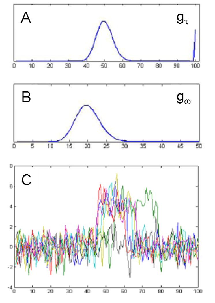
Illustration of Simulation 1 (second data set). Data was simulated for M = 20 subjects and N = 200 time points. (A) The onsets for the first 15 subjects were drawn from a Poisson distribution with mean 10. The onset times were thereafter shifted 50 time points. The remaining 5 subjects were assumed to have no activation. (B) The distribution for the duration followed a Poisson distribution with mean 20. (C) Example time courses with change points sampled from the distributions shown in (A) and (B). Note 25% of the subjects showed no activation.
The multi-subject change point estimation procedure was applied to all three data sets. Estimates of gτ and gω were computed using the standard MLE (henceforth denoted MLE), the penalized maximum likelihood method (MPLE) with penalty terms preset to h = .005 and k = 5 and the smoothed EM-algorithm (EMS) using the smoothing kernel from (8) with j = 2. This whole procedure was repeated 100 times. After each repetition, the Kullback-Leibler divergence between the true and estimated values of gτ were computed. The same procedure was repeated for gω. This allowed us to quantify the similarity between the estimated distributions and their true values.
Simulation 2
To assess the effectiveness of our multi-stage analysis procedure, images of size 40 × 40 were simulated. The images are grouped into 3 activation clusters in which the locations of shifts into and out of the activated state were drawn randomly from common (by region) distributions for onset and duration. The simulated images contain multiple regions with homogeneous distributions of timing parameters amid voxels with no activation, see Fig. 4. Noise was added to the simulated images corresponding to SNRs of .5, 1, and 2. HEWMA was applied to each of the three sets of functional data and significant voxels (p < 0.01) were moved to the second stage of the analysis. Estimates of gτ and gω were computed for these voxels using the MLE, the EMS with j = 2, and the MPLE with penalty terms h and k determined using leave-one-out cross-validation. Images were segmented with the HMRF clustering algorithm, using the expected values and standard deviations of the estimated gτ(k) and gω(k) and the differences in means between the activated and inactivated states as observed data (i.e. p = 5). The appropriate number of clusters was determined in each case using the AIC-criterion.
Figure 4.
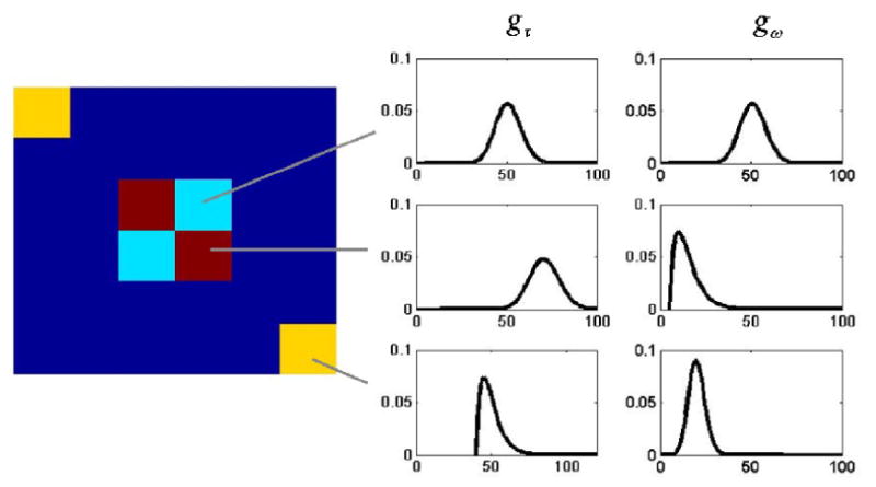
Illustration of Simulation 2. Time courses for the dark red, light blue and yellow voxels are generated using the distributions for activation onset and duration shown at the right. Dark blue voxels consist of noise time courses with no activation.
3.2 Experimental data
We applied our methods to data from 24 participants scanned with BOLD fMRI at 3T (GE, Milwaukee, WI). The experiment was conducted in accordance with the Declaration of Helsinki and was approved by the University of Michigan institutional review board. The task used was a variant of a well-studied laboratory paradigm for eliciting anxiety (Dickerson and Kemeny, 2004; Gruenewald, Kemeny, Aziz, and Fahey, 2004; Roy, Kirschbaum, and Steptoe, 2001), shown in Fig. 5. The design was an off-on-off design, with an anxiety-provoking speech preparation task occurring between lower-anxiety resting periods. Participants were informed that they were to be given two minutes to prepare a seven-minute speech, and that the topic would be revealed to them during scanning. They were told that after the scanning session, they would deliver the speech to a panel of expert judges, though there was “a small chance” that they would be randomly selected not to give the speech. After the start of fMRI acquisition, participants viewed a fixation cross for 2 min (resting baseline). At the end of this period, participants viewed an instruction slide for 15 s that described the speech topic, which was to speak about “why you are a good friend”. The slide instructed participants to be sure to prepare enough for the entire 7 min period. After 2 min of silent preparation, another instruction screen appeared (a relief instruction, 15 s duration) that informed participants that they would not have to give the speech. An additional 2 min period of resting baseline followed, which completed the functional run. Heart rate was monitored continuously, and heart rate increased after the topic presentation, remained high during preparation, and decreased after the relief instruction. Because this task involves a single change in state, as in some previous fMRI experiments (Breiter and Rosen, 1999; Eisenberger, Lieberman, and Williams, 2003), and the precise onset time and time course of subjective anxiety are unknown, this design is a good candidate for our change point analysis.
Figure 5.
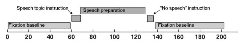
The experimental paradigm. Participants were told they would silently prepare a speech under high time pressure during fMRI scanning, which they would subsequently give in front of a panel after the session. They were informed of the topic via visual presentation after 2 min of baseline scanning. After 2 min of speech preparation, they were informed (visually) that they would not have to give a speech after all, and they rested quietly for the final 2 min of scanning.
A series of 215 images were acquired using a T2*-weighted, single-shot reverse spiral acquisition (gradient echo, T = 2000, TE = 30, flip angle = 90) with 40 sequential axial slices (FOV = 20, 3.12 × 3.12 × 3 mm, skip 0, 64 × 64 matrix). This sequence was designed to enable good signal recovery in areas of high susceptibility artifact, e.g. orbitofrontal cortex. High-resolution T1 spoiled gradient recall (SPGR) images were acquired for anatomical localization and warping to standard space.
Offline image reconstruction included correction for distortions caused by magnetic field inhomogeneity. Images were corrected for slice acquisition timing differences using a custom 4-point sync interpolation and realigned (motion corrected) to the first image using Automated Image Registration (AIR; (Woods, Grafton, Holmes, Cherry, and Mazziotta, 1998)). SPGR images were coregistered to the first functional image using a mutual information metric (SPM2). When necessary, the starting point for the automated registration was manually adjusted and re-run until a satisfactory result was obtained. The SPGR images were normalized to the Montreal Neurological Institute (MNI) single-subject T1 template using SPM2 (with the default basis set). The warping parameters were applied to functional images, which were then smoothed with a 9 mm isotropic Gaussian kernel. Individual-subject data were subjected to linear detrending across the entire session (215 images) and analyzed with EWMA. An AR(2) model was used to calculate the EWMA statistic and its variance, and they were both carried forward to the group level HEWMA analysis. We used custom software to calculate statistical maps throughout the brain, including HEWMA (group) t and p-values for activations (increases from baseline) and deactivations (decreases from baseline).
Significant voxels (p < 0.01) were brought forth to the next level of analysis, where the distribution of onset and duration were estimated using the penalized maximum likelihood method with penalty terms h and k determined using leave-one-out cross-validation. Next, images were segmented with the HMRF clustering algorithm, using the expected values and standard deviations of the estimated gτ(k) and gω(k) and the differences in means between the activated and inactivated states as observed data. The number of clusters was determined using the AIC-criterion. Finally, for each cluster the estimates of the distribution of onset and duration were combined to cluster-wise estimates and the probability of activation as a function of time was estimated for each cluster.
4 Results
4.1 Simulations
Simulation 1
The KL-divergence was used to assess the difference between the estimated values of gτ(t) and gω(k) and the true distributions used to create the simulations. The results for gτ(t) are shown in Fig. 6. Analogous results for gω(k), not presented here, gave rise to similar results. The left column shows the 3 distributions used to generate the subject-specific onset times. The center and right columns show boxplots of the estimated KL-divergence between the true and estimated value of gτ(t) for 100 different repetitions of the simulation obtained using the MLE and MPLE approaches, respectively. Results for the EMS approach produced similar results to the MLE and are not presented here. Each set of simulations were repeated using 3 different SNRs. It is clear from studying the boxplots that when the SNR is low (e.g., 0.5), the MLE approach gives rise to extremely variable estimates of the true onset distribution. The estimates improve as the SNR increases. These results are consistent with empirical evidence showing that for low SNR values the MLE estimation gives rise to noisy and rough estimates that are ill-suited for estimating the true underlying distribution which is smooth. The MPLE approach performs consistently better than the MLE, particularly at low SNR. This is not surprising as these estimates not only reflect the shape of the true underlying distribution but also its smoothness properties.
Figure 6.
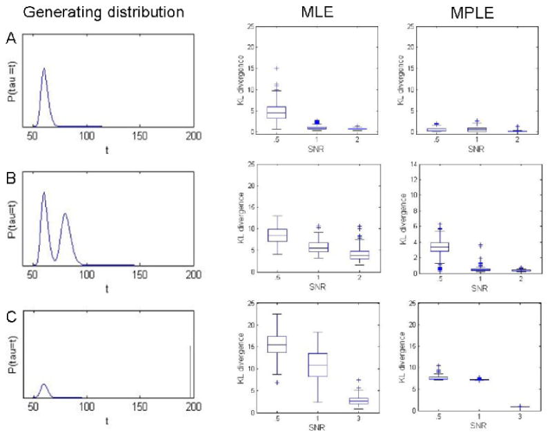
Results of Simulation 1. The left column shows the true value of gτ for the three simulated data sets. Note that the bottom right figure represents a distribution with positive (.25) probability of no activation, indicated by mass at the end of the time course. The center column shows box plots of the KL-divergence between the true and estimated onset distributions at three different SNR levels, with estimates computed using the MLE approach. The right column shows similar results for the MPLE approach. Clearly the inclusion of the penalty term gives rise to closer fits and therefore smaller KL-divergences.
Results varied according to the shape of the generating distribution. For a simple unimodal distribution (Fig. 6A), the MPLE gave consistently accurate results for all SNR levels. However, as the generating distribution became more complicated the difference in accuracy between low and high SNR became more apparent. This was particularly true for the distribution where some subjects showed no reaction (Fig. 6C).
Simulation 2
HEWMA analysis was performed on each data set and voxels deemed significant (p < 0.01) were moved to the second stage of analysis. For these voxels, estimated clusters were computed using our spatial clustering algorithm with observed data obtained using both the MLE and the MPLE approach. Results using data obtained with the EMS approach produced similar results to the MLE and are not presented here. Results for three different SNR levels are shown in Fig. 7. In each case the AIC-criterion correctly picked 3 clusters of activation. For the MLE approach the ability of the clustering algorithm to correctly classify regions is adversely effected by decreases in SNR. This effect is much less pronounced when using observations obtained via the MPLE approach. Both these results are consistent with those found in Simulation 1, as the noisy estimates of the distribution of onset and duration obtained using the MLE method would appear to be ill-suited to use for clustering purposes.
Figure 7.
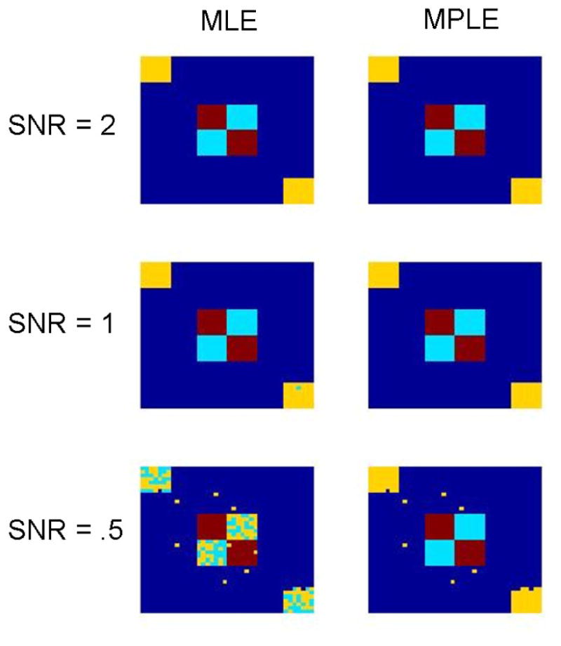
Results of Simulation 2. Using the results of our change-point methods, simulated images were segmented into spatial clusters. For low SNRs, clustering based on the results of the MPLE approach performed significantly better than the MLE approach.
In general, our simulations indicate that the MPLE approach gives the most accurate estimates of the true underlying distributions that generated the observed change points. For these reasons, we strongly recommend using the MPLE approach over the MLE and EMS approaches unless the SNR of the data is high.
4.2 Experimental data
A full description of the results of the HEWMA analysis can be found in previous work (Lindquist, Waugh, and Wager, 2007; Lindquist and Wager, 2008). Here we instead concentrate on results relating directly to the change point/spatial clustering framework developed in this paper. The results for a single slice are presented in Figs. 8-9. The HEWMA analysis passed through 5 spatially coherent regions of activation consisting of 301 voxels. For each of these voxels, the MPLE estimation procedure was performed and the results were spatially clustered. The analysis revealed four coherent clusters of activation (see Fig. 8). Fig. 9 shows the estimated distributions of onset and duration averaged across all voxels contained in each of the clusters. The average probability of activation was calculated for each cluster, as was the probability of elevated heart rate (Fig. 8).
Figure 8.
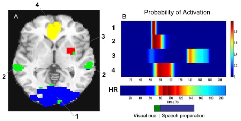
(A) The brain is split into 4 clusters of spatially coherent activation. (B) The estimated probability of activation is shown in a heat map for each of the four clusters. In addition the probability of elevated heart rate (HR) is shown. The timing of the original visual cue and the speech preparation is shown in block format on the bottom right hand side for comparison purposes. Activation in the ventromedial prefrontal cortex (Cluster 4) correlates highly with heart-rate increases in the task.
Figure 9.
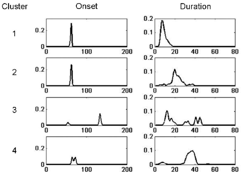
The estimated distributions for onset and duration are shown for each of the four clusters defined in Fig. 8. The results are averaged across all voxels contained in each cluster. These distributions are used to calculate the probability of activation presented in Fig. 8.
Results indicate that the visual cortex (blue in Fig. 8) has high probability of being activated during the presentation of the visual cue (as expected). The ventral striatum (red in Fig. 8) has a high probability of activation after the relief cue was given, indicating this region may be associated with relief. The superior temporal cortices (green) associated in social neuroscience studies with inferences about agency, among other things, showed evidence of activation during the first part of the speech preparation task. Finally, the ventromedial prefrontal cortex (yellow), an area associated with visceromotor control, self-related attention, and generation and regulation of emotion based on context was the only area to show sustained activation during speech preparation. Activation in this region correlated highly with heart-rate increases in the task (Wager, Waugh, Lindquist, Noll, Fredrickson, and Taylor, 2009b).
The results show how the HEWMA analysis with activation probability estimation can identify brain regions with different relationships to task performance. Because of differences in onsets and durations, these activations could not be easily detected using the widely adopted GLM framework.
5 Discussion
In this work we introduce a technique for studying state-related single epoch paradigms, which we apply to an fMRI study of state anxiety. The data analysis was performed in a three step procedure. In the first stage we employed HEWMA (Hierarchical EWMA) (Lindquist, Waugh, and Wager, 2007; Lindquist and Wager, 2008), as a simple screening procedure to determine which voxels have time courses that deviate from a baseline level and should be moved into the next stage of the analysis. Once a systematic deviation from baseline was detected, the second step in the analysis entailed estimating when exactly the change took place, as well as the recovery time (if any). We estimated voxel-specific distributions of onset times and durations from the fMRI response, by modeling each subjects onset and duration as random variables drawn from an unknown population distribution. We estimated these distributions assuming no functional form, and allowing for the possibility that some subjects may show no response. Finally, we performed spatial clustering of voxels according to onset and duration characteristics, and anatomical location using a hidden Markov random field model. This three step procedure provides a general spatio-temporal model for dealing with data with uncertain onset and duration. Earlier work (Lindquist, Waugh, and Wager, 2007; Lindquist and Wager, 2008) introduced the HEWMA procedure, as well as a simple approach towards performing the latter two steps of the analysis which employed a finite mixture model and k-means clustering, respectively. The current paper is concerned with introducing improved methods for performing these two latter steps; relaxing the assumption that all subjects have the same onset and duration of activation and incorporating spatial considerations into the clustering algorithm.
While the whole analysis procedure outlined above could reasonably be combined into a single model, it would be complicated and computationally expensive to fit. We propose the multi-stage approach as a stop-gap solution until a single spatio-temporal model is feasible. Simulations indicate that the multi-stage approach provides an adequate balance between computational costs and efficiency. A weakness of the proposed approach is the fact that the parameter estimates between steps are treated as data, measured without error. This comes with certain risk of increased bias due to the propagation of errors through various steps of the analysis. In the current context, reducing data using HEWMA may result in inflated false positives and false negatives (i.e. voxels may be moved to the second stage that ought not and voxels that aren't moved may have mistakenly been left behind, thus biasing results).
It is important to note that the HEWMA stage of the analysis is simply used to locate voxels of interest and can be replaced by an alternative data reduction technique or excluded altogether. In the latter case the change point methodology could be applied directly to every voxel in the brain. However, the computational costs would be high and we find the use of an initial data reduction procedure to be beneficial. As an alternative to HEWMA, the change point methodology could be applied directly to data from ROI studies or to temporal components obtained from a PCA or ICA analysis. Alternatively, the combined change point/spatial clustering technique could be applied to voxels deemed active in a mediation analysis (Wager, Davidson, Hughes, Lindquist, and Ochsner, 2008).
The change point methods developed in this paper are appropriate for group fMRI data, particularly for studies when it is not possible to replicate experimental manipulations within subjects (e.g., a state anxiety induction that cannot be repeated without changing the psychological nature of the state). Emotional responses are one prime candidate for application of the method. Others include identifying voxels of interest and characterizing brain responses in ‘ecologically valid’ tasks, changes in state-related activity evoked by learning, or to studies of tonic increases following solutions to ‘insight’ problem-solving tasks. Still another interesting application is longitudinal studies of brain function or structure, and how they change with development or with the progression of a neurological or psychiatric disorder. In general, our proposed approach may be particularly useful for arterial spin labeling and per-fusion MRI studies, which measure brain activity over time without the complicating factors of signal drift and highly colored noise found in fMRI (Liu, Wong, Frank, and Buxton, 2002; Wang, Rao, Wetmore, Furlan, Korczykowski, Dinges, and Detre, 2005).
Currently the model is designed to handle a single state-related shift from a baseline to activated state and a subsequent return to baseline at a later unknown time. This type of model is suited for studying state-related single epoch paradigms. The current approach does not readably extend to event-related paradigms, as it only allows for a single activation and it does not directly take information about the hemodynamic response into consideration. The model could potentially be generalized for other situations, including more rapid alteration among multiple states. One possible extension is to allow for the possibility of multiple activation onsets and durations though out the course of the time series. This can be done by extending the likelihood function defined in (1) and (2) to allow for multiple returns to the active state at unique time points, and the problem would extend to estimating distributions for multiple onsets and durations. Though the extension of the likelihood function and the resulting EM-algorithm used to estimate these multiple distributions would appear relatively straight forward, it would lead to a significant increase in computational costs. In addition, there may be particular confounds if the response is non-linear which will mean that simply adding extra parameters to the likelihood will not necessarily give the same form of the distributions. Finally, the conditional nature of change points in this situation may complicate matters even further. Another possible extension relates to the number of states included in the model. In certain applications it may be desirable to extend the model to allow for different baseline means before and after activation, thereby necessitating a three-state model. This can be done within our current model formulation by exchanging the last term in the product of (1) by f(yij, θ3) where θ3 = (μ3, , i = 1 … M) represents the parameters associated with the second baseline period.
Our model makes a number of assumptions, namely that the data is independent identically distributed within states and that state means are equal across subjects. While it is generally assumed that fMRI data is autocorrelated, we make the independence assumption to simplify computation. There remains the option to pre-whitened the data prior to analysis (Woolrich, Ripley, Brady, and Smith, 2001), though as data used for this type of model tend to have a strong low frequency component special care must be taken to avoid removing signal from the data. The method could alternatively be generalized to handle colored noise, by incorporating a covariance matrix corresponding to an autocorrelation model (e.g. AR(p) or ARMA(1,1)) in the likelihood function shown in (1).
The spatial clustering algorithm can be extended by using an inhomogeneous model that implies that some neighbor pairs have a greater degree of spatial dependence than others. These types of models are therefore useful in preserving edges between regions of high contrast and are often used as priors in Bayesian image analysis (Brezger, Fahrmeir, and Hennerfeind, 2007; Aykroyd and Zimeras, 1999). In our application we could also employ information from the time domain, or from prior anatomical knowledge in specifying the degree of spatial smoothness between voxels. If information on the degree of temporal correlation or regions of grey/white matter is available, it can also be incorporated into the image model.
Acknowledgments
We would like to thank Doug Noll, Stephan F. Taylor, Barbara Fredrickson, and Luis Hernandez for providing the data set used in this paper. MATLAB code implementing the methods described in this paper is freely available by contacting the authors.
Appendix
A. EM algorithm for the MLE approach
E-step: Given the current estimates at the tth step, , , and , estimate the M × (N − ωmax + 1) × (ωmax − ωmin + 1) matrix Z, whose elements zijk represent the probability that subject i has change points τi = j and ωi = k, conditional on the data Y and the current parameter estimates. Let
| (22) |
Then the elements of Z are given by
| (23) |
| (24) |
M-step: Given zijk update the parameter estimates.
| (25) |
| (26) |
| (27) |
| (28) |
| (29) |
where
| (30) |
B. EM-algorithm for the MPLE approach
In the penalized version of the EM-algorithm, a smoothness penalty λJ(gτ, gω) is placed on the unknown population distributions gτ and gω. Both the E-step and the M-Step estimates of μ and σ remain the same as in the EM-algorithm described in Appendix A. Computing and becomes more complicated, as there is no closed-form solution to the M-step update equation after the addition of the penalty term. The (N − ωmin)-dimensional system of equations for updating the parameters ητ = (ητ(1), ητ(2), …, ητ(τmax))′ from (5) is
| (31) |
where 0 and 1 are vectors of zeros and ones, respectively, Σ is as given in (7), and g( η τ) = (g(1|ητ), g(2|ητ), …, g(τmax|ητ))′ as in (5). As the M-step estimates cannot be computed directly, we employ a variation of the EM-algorithm, called the Generalized EM-algorithm ((McLachlan and Krishnan, 2007)). Here an optimization algorithm is used to iteratively compute in the M-step. To ensure that the algorithm moves closer to the MLE it is not necessarily to find the root of (31) in each M-step, but simply move towards it. Thus, we can implement a pre-specified number of steps of a numerical optimization algorithm such as Newton-Raphson, and even if we do not reach convergence within the M-step, the Generalized EM-algorithm should converge to the MLE.
Footnotes
Publisher's Disclaimer: This is a PDF file of an unedited manuscript that has been accepted for publication. As a service to our customers we are providing this early version of the manuscript. The manuscript will undergo copyediting, typesetting, and review of the resulting proof before it is published in its final citable form. Please note that during the production process errors may be discovered which could affect the content, and all legal disclaimers that apply to the journal pertain.
References
- Akaike H. Information theory and an extension of the maximum likelihood principle. Proc of the 2nd Int Symp on Information Theory. 1973:267–281. [Google Scholar]
- Beckmann CF, Smith SM. Probabilistic independent component analysis for functional magnetic resonance imaging. EEE Transactions on Medical Imaging. 2004;23:137–152. doi: 10.1109/TMI.2003.822821. [DOI] [PubMed] [Google Scholar]
- Besag J. Spatial interaction and the statistical analysis of lattice systems. Journal of the Royal Statistical Society, Series B. 1974;36:179–195. [Google Scholar]
- Bishop CM. Pattern Recognition and Machine Learning (Information Science and Statistics) Springer; 2006. [Google Scholar]
- Breiter HC, Gollub RL, Weisskoff RM, Kennedy DN, Makris N, Berke JD, Goodman JM, Kantor HL, Gastfriend DR, Riorden JP, Mathew RT, Rosen BR, Hyman SE. Acute effects of cocaine on human brain activity and emotion. Neuron. 1997;19(3):591–611. doi: 10.1016/s0896-6273(00)80374-8. [DOI] [PubMed] [Google Scholar]
- Breiter Hc, Rosen BR. Functional magnetic resonance imaging of brain reward circuitry in the human. Ann N Y Acad Sci. 1999;877:523–547. doi: 10.1111/j.1749-6632.1999.tb09287.x. [DOI] [PubMed] [Google Scholar]
- Calhoun VD, Adali T, Pearlson G, Pekar J. Spatial and temporal independent component analysis of functional mri data containing a pair of task-related waveforms. Human Brain Mapping. 2001;13:43–53. doi: 10.1002/hbm.1024. [DOI] [PMC free article] [PubMed] [Google Scholar]
- Calhoun VD, Stevens MC, Pearlson GD, Kiehl KA. fMRI analysis with the general linear model: removal of latency-induced amplitude bias by incorporation of hemodynamic derivative terms. NeuroImage. 2004;22:252–257. doi: 10.1016/j.neuroimage.2003.12.029. [DOI] [PubMed] [Google Scholar]
- Dempster AP, Laird NM, Rubin DB. Maximum-likelihood from incomplete data via the EM algorithm. Journal of Royal Statistical Society B. 1977;39:1–38. [Google Scholar]
- Dickerson SS, Kemeny ME. Acute stressors and cortisol responses: a theoretical integration and synthesis of laboratory research. Psychol Bull. 2004;130:355–391. doi: 10.1037/0033-2909.130.3.355. [DOI] [PubMed] [Google Scholar]
- Eisenberger NI, Lieberman MD, Williams KD. Does Rejection Hurt? An fMRI Study of Social Exclusion. Science. 2003;302(5643):290–292. doi: 10.1126/science.1089134. [DOI] [PubMed] [Google Scholar]
- Friston KJ, Fletcher P, Josephs O, Holmes A, Rugg MD, Turner R. Event-related fmri: characterizing differential responses. NeuroImage. 1998;7:30–40. doi: 10.1006/nimg.1997.0306. [DOI] [PubMed] [Google Scholar]
- Geman S, Geman D. Stochastic relaxation, gibbs distributions, and the bayesian restoration of images. I E E E Trans Pattern Anal Machine intell. 1984;6:721–741. doi: 10.1109/tpami.1984.4767596. [DOI] [PubMed] [Google Scholar]
- Glover GH. Deconvolution of impulse response in event-related BOLD fMRI. NeuroImage. 1999;9(4):416–429. doi: 10.1006/nimg.1998.0419. [DOI] [PubMed] [Google Scholar]
- Gruenewald TL, Kemeny ME, Aziz N, Fahey JL. Acute threat to the social self: shame, social self-esteem, and cortisol activity. Psychosom Med. 2004;66:915–924. doi: 10.1097/01.psy.0000143639.61693.ef. [DOI] [PubMed] [Google Scholar]
- Joseph J, Wolfson DB. Maximum likelihood estimation in the multipath changepoint problem. Annals of the Institute of Statistical Mathematics. 1993;45:511–530. [Google Scholar]
- Lindquist MA, Loh J, Atlas L, Wager TD. Modeling the hemodynamic response function in fmri: Efficiency, bias and mis-modeling. NeuroImage. 2008;45:S187–S198. doi: 10.1016/j.neuroimage.2008.10.065. [DOI] [PMC free article] [PubMed] [Google Scholar]
- Lindquist MA, Wager TD. Validity and power in hemodynamic response modeling: A comparison study and a new approach. Human Brain Mapping. 2007;28:764–784. doi: 10.1002/hbm.20310. [DOI] [PMC free article] [PubMed] [Google Scholar]
- Lindquist MA, Wager TD. Application of change-point theory to modeling state-related activity in fmri. In: Cohen P, editor. Applied Data Analytic Techniques for “Turning Points” Research. Mahwah, NJ: Lawrence Erlbaum Associates Publishers; 2008. [Google Scholar]
- Lindquist MA, Waugh C, Wager TD. Modeling state-related fMRI activity using change-point theory. NeuroImage. 2007;35:1125–1141. doi: 10.1016/j.neuroimage.2007.01.004. [DOI] [PubMed] [Google Scholar]
- Liu TT, Wong EC, Frank LR, Buxton RB. Analysis and design of perfusion-based event-related fmri experiments. NeuroImage. 2002;16:269–282. doi: 10.1006/nimg.2001.1038. [DOI] [PubMed] [Google Scholar]
- Loh J, Lindquist MA, Wager TD. Residual analysis for detecting mis-modeling in fmri. Statistica Sinica. 2008;18:1421–1448. [Google Scholar]
- McKeown MJ, Makeig S. Analysis of fmri data by blind separation into independant spatial components. Human Brain Mapping. 1998;6:160–188. doi: 10.1002/(SICI)1097-0193(1998)6:3<160::AID-HBM5>3.0.CO;2-1. [DOI] [PMC free article] [PubMed] [Google Scholar]
- McLachlan GJ, Krishnan T. The EM Algorithm and Extensions (Wiley Series in Probability and Statistics) Wiley-Interscience; 2007. [Google Scholar]
- Potts RB. Some generalized order-disorder transformations. Proceedings of the Cambridge Philosophical Society. 1952;48:106–109. [Google Scholar]
- Roy MP, Kirschbaum C, Steptoe A. Psychological, cardiovascular, and metabolic correlates of individual differences in cortisol stress recovery in young men. Psychoneuroendocrinology. 2001;26(4):375–391. doi: 10.1016/s0306-4530(00)00061-5. [DOI] [PubMed] [Google Scholar]
- Silverman B, Jones M, Wilson J, Nychka D. A smoothed em approach to indirect estimation problems with particular reference to sterology and emission tomography. Journal of the Royal Statistical Society, Series B. 1990;52:271–324. [Google Scholar]
- Silverman BW. Density Estimation for Statistics and Data Analysis. Chapman & Hall/CRC; Apr, 1986. [Google Scholar]
- Swendsen R, Wang J. Nonuniversal critical dynamics in monte carlo simulations. Physical Rev. Letters. 1987;58:86–88. doi: 10.1103/PhysRevLett.58.86. [DOI] [PubMed] [Google Scholar]
- Wager TD, Davidson ML, Hughes BL, Lindquist MA, Ochsner KN. Prefrontal-subcortical pathways mediating successful emotion regulation. Neuron. 2008;59:1037–1050. doi: 10.1016/j.neuron.2008.09.006. [DOI] [PMC free article] [PubMed] [Google Scholar]
- Wager TD, van Ast V, Hughes BL, Davidson ML, Lindquist MA, Ochsner KN. Brain mediators of cardiovascular responses to social threat, part ii: Prefrontal subcortical pathways and relationship with anxiety. Submitted to NeuroImage. 2009a doi: 10.1016/j.neuroimage.2009.05.044. [DOI] [PMC free article] [PubMed] [Google Scholar]
- Wager TD, Waugh C, Lindquist MA, Noll DC, Fredrickson BL, Taylor SE. Brain mediators of cardiovascular responses to social threat, part i: Reciprocal dorsal and ventral sub-regions of the medial prefrontal cortex and heart-rate reactivity. Submitted to NeuroImage. 2009b doi: 10.1016/j.neuroimage.2009.05.043. [DOI] [PMC free article] [PubMed] [Google Scholar]
- Wang J, Rao H, Wetmore GS, Furlan PM, Korczykowski M, Dinges DF, Detre J. Perfusion functional mri reveals cerebral blood flow pattern under psychological stress. Proc Natl Acad Sci U S A. 2005;102(3):17804–17809. doi: 10.1073/pnas.0503082102. [DOI] [PMC free article] [PubMed] [Google Scholar]
- Wise RG, Williams P, Tracey I. Using fmri to quantify the time dependence of remifentanil analgesia in humans. Neuropsychopharmacology. 2004;29(3):626–635. doi: 10.1038/sj.npp.1300364. [DOI] [PubMed] [Google Scholar]
- Woods RP, Grafton ST, Holmes CJ, Cherry SR, Mazziotta JC. Automated image registration: I. general methods and intrasubject, intramodality validation. Journal of Computer Assisted Tomography. 1998;22(1):139–152. doi: 10.1097/00004728-199801000-00027. [DOI] [PubMed] [Google Scholar]
- Worsley KJ, Friston KJ. Analysis of fMRI time-series revisited-again. NeuroImage. 1995;2:173–181. doi: 10.1006/nimg.1995.1023. [DOI] [PubMed] [Google Scholar]
- Zhang X, Johnson T, Little R, Cao Y. Quantitative magnetic resonance image analysis via the em algorithm with stochastic variation. Annals of Applied Statistics. 2008;2:736–755. doi: 10.1214/07-AOAS157. [DOI] [PMC free article] [PubMed] [Google Scholar]
- Zhang Y, Brady M, Smith S. Segmentation of brain mr images through a hidden markov random field model and the expectation-maximization algorithm. I E E E Trans Medical Imag. 2001;20:721–741. doi: 10.1109/42.906424. [DOI] [PubMed] [Google Scholar]