

Abstract
Over 40 years ago, Hubel and Wiesel gave a preliminary report of the first account of cells in monkey cerebral cortex selective for binocular disparity. The cells were located outside of V-1 within a region referred to then as “area 18.” A full-length manuscript never followed, because the demarcation of the visual areas within this region had not been fully worked out. Here, we provide a full description of the physiological experiments and identify the locations of the recorded neurons using a contemporary atlas generated by functional magnetic resonance imaging; we also perform an independent analysis of the location of the neurons relative to an anatomical landmark (the base of the lunate sulcus) that is often coincident with the border between V-2 and V-3. Disparity-tuned cells resided not only in V-2, the area now synonymous with area 18, but also in V-3 and probably within V-3A. The recordings showed that the disparity-tuned cells were biased for near disparities, tended to prefer vertical orientations, clustered by disparity preference, and often required stimulation of both eyes to elicit responses, features strongly suggesting a role in stereoscopic depth perception.
Keywords: binocular vision; depth; extrastriate cortex; functional organization; Hubel and Wiesel, stereopsis
Introduction
A hallmark of animals with frontal-facing eyes such as cats and primates is their ability to extract stereoscopic depth information from the disparity in the 2-dimensional images projected on each retina (Wheatstone 1838; Bough 1970; Fox and Blake 1971). Primary visual cortex (V-1 or area 17) is the first stage along the central visual pathway at which single neurons receive input from both eyes and could therefore compute stereoscopic depth. Neurons in V-1 with receptive fields having disparate positions in the 2 retinas were first described in the anesthetized cat by Pettigrew and colleagues (Barlow et al. 1967; Pettigrew et al. 1968). These investigators used an adjustable prism in front of one eye to vary the relative directions of gaze of the 2 eyes, and found cells that responded maximally to stimuli in front of, behind, or at the plane of fixation of the animal.
The search for disparity-selective neurons in monkey V-1 was initially unsuccessful (Hubel and Wiesel, personal communication), prompting an exploration of extrastriate cortex. The first account of disparity-tuned neurons in monkey was given in a brief report in 1970 (Hubel and Wiesel 1970), but was never followed by a full-length manuscript. Subsequent studies have described disparity-tuned neurons within a number of extrastriate areas, including V-2, V-3, V-3A, V-5/MT (middle temporal area), V-4, and inferior temporal cortex (Poggio and Fischer 1977; Hubel and Livingstone 1987; Poggio et al. 1988; DeAngelis and Newsome 1999; Adams and Zeki 2001; Hegdé and Van Essen 2005; Verhoef et al. 2010; Anzai et al. 2011). Evidence for disparity-tuned cells in V-1 of primates is also now unequivocal (Poggio et al. 1988; Cumming and Parker 1997; Bakin et al. 2000; Cumming and DeAngelis 2001).
The reader might reasonably wonder about the reasons for the unusually long gap between the date (1968–1970) when the single-unit recordings described here were done and now the presentation of a full-length paper, almost half a century later. Certainly in the interim there have been many technical developments, such as the invention of digital recording devices that have afforded much more detailed quantitative assessments. The main reason why the unpublished results were put on the shelf was the difficulty in identifying the visual area(s) in which the recordings were made. While the border between V-1 and V-2 is in macaque and man razor sharp, any cytoarchitectonic borders beyond (anterior to) this boundary are hard to identify in Nissl-stained sections. The depth-sensitive cells were clearly outside of striate cortex; out of ignorance of any further functional segregation in extrastriate cortex, the location of the recordings was simply assigned to “area 18.” Functional subdivisions of what was then poorly described terrain have become clear using a range of anatomical and functional techniques (Van Essen and Zeki 1978; Ungerleider and Desimone 1986; Hubel and Livingstone 1987; Hof and Morrison 1995; Lewis and Van Essen 2000), including functional magnetic resonance imaging (fMRI; Logothetis et al. 1999; Fize et al. 2003). The functional subdivisions of the retinotopic brain areas adjacent to striate cortex, including V-2, V-3, and V-3A, are now reasonably well worked out (Paxinos et al. 2000; Van Essen and Dierker 2007).
Since it might be of some historical interest, we present Hubel and Wiesel's original unpublished single-cell results describing the properties of the disparity-tuned neurons and the most likely areas of their location. The locations were determined by aligning histological sections containing the original electrode penetrations with a contemporary functional atlas of the visual areas of macaque. We also analyzed the cell locations relative to an anatomical landmark, the base of the lunate sulcus, which is often coincident with the border between V-2 and V-3. In some cases, the identification of the recordings was facilitated by close examination of remastered film footage captured during the experiments (see Supplementary Movies). The physiological recordings provide a confirmation of a number of observations made using more sophisticated techniques, especially the preponderance and local clustering of disparity-tuned neurons in V-2, V-3, and V-3A (Bakin et al. 2000; Adams and Zeki 2001; Ts'o et al. 2001; Thomas et al. 2002; Anzai et al. 2011).
Results
Disparity Tuning of Example Cells
Single neurons were recorded in anesthetized macaque monkey visual cortex with tungsten microelectrodes (Hubel 1957). The electrode penetrations entered the brain on the dorsal aspect, just posterior to the lunate sulcus (“business electrode” Fig. 1). For most of the experiments, the penetrations proceeded from the point of entry through the buried annectant gyrus (see green bump in Fig. 3B). Tests were made to determine each neuron's orientation selectivity, binocularity, and binocular disparity. Slow drifts in eye alignment were controlled by aligning the gaze direction of the 2 eyes by way of a prism in front of the left eye. Alignment was assessed by mapping a V-1 receptive field in the 2 eyes separately (“tag” cell, Fig. 1). Any well-isolated binocular neuron in V-1 with a small receptive field could serve as a tag cell. The technique relies on the assumption that, under natural viewing with aligned eyes, the receptive fields in each eye also align. In retrospect, the use of a V-1 cell to monitor eye alignments could have introduced some error since many V-1 neurons have since been shown to possess disparity tuning (Poggio et al. 1988; Cumming and Parker 1997; Bakin et al. 2000; Cumming and DeAngelis 2001). This technique would therefore introduce a bias in the measurement of disparity, equal to the disparity of the V-1 tag cell used during a given experiment. This bias would be expected to be relatively small in comparison with the disparity tuning measured in the majority of neurons, since V-1 disparity-tuned neurons have small spatial offsets in the receptive field locations measured in the 2 eyes (on the order of ∼0.1°; Tsao, Conway, et al. 2003). Bars of light to map the receptive fields were generated with a hand-held slide projector aimed at the tangent screen; in a few later experiments, stimuli were programmed with a computer and displayed on a cathode ray tube monitor. After a tag-cell was isolated, the prism was adjusted to bring the receptive field location measured in the left eye alone (i.e. with the right eye masked) into register with the receptive field measured in the right eye alone, thus bringing the eyes into alignment. The prism setting was directly displayed on the screen by projecting through the prism a laser beam reflected toward the screen by an angled mirror adjacent to the left eye (Fig. 1). The location of the beam when the 2 eyes were aligned was marked on the screen. The screen was also marked along the horizontal axis to indicate fractions of a degree of disparity obtained by various prism settings, with near disparities to the left and far (or distant) disparities to the right of alignment (Fig. 2A). This technique made it possible to rapidly assess and correct gaze direction, and to measure disparity tuning. A single tag cell was held for long durations, often the duration of an experiment, providing a constant reference.
Figure 1.

Bird's eye view of the recording set-up for measuring disparity tuning in macaque extrastriate cortex. See Results and Methods for details.
Figure 3.

Reconstruction of electrode penetrations. (A) Low-power, Nissl-stained sagittal section from the experiment run on 24 June 1969. Black arrow shows the area 17/area 18 border. Electrode tract has been drawn on the tracing of the section. The tracing of the cortex within the boxed region of (A) is shown in (B), superimposed on the corresponding MRI macaque atlas section showing area designations. The MRI atlas was generated using different animals from those used in the physiology experiments; the atlas was made by conducting a functional scan of retinotopy to identify area borders (e.g., see Fize et al. 2003). (C) high-resolution Nissl-stained section corresponding to the boxed region in (B), containing the 3 electrolytic lesions made during the recording (arrows). (D) Cell identifications reconstructed on the electrode tract. Red dashes indicate disparity-tuned neurons.
Figure 2.

Responses of 2 disparity-tuned neurons recorded on 24 June 1969 in what is now known to be V-2 (see Fig. 3). (A) Cell 31, receptive field map. Diagram at the bottom shows the laser beam coordinates of gaze directions indicating aligned eyes, near disparities, and far (distant) disparities. (The dark horizontal band across the page is an acid stain caused by 43-year-old masking tape.) The neuron's peak tuning is indicated in pencil. (B) Cell 31, disparity-tuning curve; squares show responses to single-eye stimulation (solid, right; open, left). (C) Cell 20, responses to horizontal disparities showing maximal activation to aligned LE and RE receptive fields. Dashed lines indicate receptive field for the left eye (LE); solid lines indicate receptive field for the right eye (RE). (D) Cell 20, disparity-tuning curve; single-eye response for each eye shown as a square symbol. Each point in the graph is the average of 10 back-and-forth passes of a computer-generated moving slit. (E) Cell 20, responses to stimulation of either eye alone (top panels), and to both eyes simultaneously (bottom panel). See Supplementary File 1; Supplementary Movies 1–6; Supplementary Figures 1 and 2.
Figure 2A shows the receptive field map of a complex cell recorded on 24 June 1969, drawn directly on the tangent screen in front of the animal. Orientation preference was mapped as previously described (Hubel and Wiesel 1962). Disparity tuning along the horizontal axis was determined simply by stimulating the neuron with an optimally oriented bar at various prism settings, and taking note of the firing rate and the location of the beam along the horizontal ruler markings. The neuron had a parafoveal receptive field (3° down, 1.8° out) with a near vertical orientation preference (10° clockwise from vertical) and was not direction selective. It showed a peak response to near disparities of approximately½ degree (Fig. 2B; Supplementary Movie 1). The neuron showed very weak response to stimulation with either eye alone (Fig. 2, solid square symbol, right eye alone; open square symbol, left eye alone; Supplementary Movie 2). A demonstration of the cell's preference for near disparities is given in Supplementary Movie 3: The prism settings were adjusted to bring the eyes into alignment, and the neuron was stimulated by waving a ruler held in a vertical orientation across the receptive field at various distances between animal and screen. (The original experimental records indicate the implement as a slide rule, which was a mistake: it was a ruler; see Supplementary Material 1 for the complete original experimental record.) The peak response was obtained at 15–20″ in front of the screen, consistent with the measured disparity preference. Disparity-tuned neurons were distinguished from nondisparity binocular neurons on the basis of the sharpness of their disparity-tuning functions. Supplementary Figure 1 shows the results for a binocular neuron that was not sensitive to the precise position of the stimulus in the 2 eyes, and was not disparity tuned. The adjudication of disparity tuning was made conservatively, on a subjective basis: neurons with frankly peaked tuning functions were deemed disparity tuned.
Figure 2C–E shows the responses for cell 20 recorded the same day. This neuron (receptive field 1.2° down, 1.3° out from fixation) also showed a preference for nearly vertically oriented bars, but was tuned to zero disparity. The sharp peak in the disparity-tuning curve distinguishes the cell from a binocular neuron lacking disparity tuning (e.g. Supplementary Fig. 1). The top row in Figure 2C shows the neural response when the image entering the left eye was deviated to the right. The spike-train record, captured by photographing the oscilloscope trace, shows only a single spike for this condition. Subsequent rows in Figure 2C show the neural responses obtained by varying the relative position of the images projected to the left and right eyes. The middle row shows the optimal configuration, with eye inputs aligned (Supplementary Movie 4). Figure 2D quantifies the neuron's disparity tuning. Like cell 31, this neuron showed little or no response to stimulation of either eye alone (solid symbol, Fig. 2D; Supplementary Movie 5). The top row in Figure 2E shows the response to a vertical bar presented to the right eye only; the middle row shows the response to the same stimulus presented to the left eye only; and the bottom row shows the responses when both eyes were open. The neuron shows a nonlinear response to combined input from the 2 eyes. The neuron whose responses are given in the figure from Hubel and Wiesel (1970) was cell 22 recorded on the same day.
Receptive fields have 2-dimensional spatial structure (Hubel and Wiesel 1962, 1968). As a result, cells could encode both horizontal and vertical disparities (Ohzawa et al. 1990; Cumming and DeAngelis 2001). This possibility was recognized: as Hubel and Wiesel (1970) described, the optimal response of extrastriate disparity-tuned neurons was usually obtained when the field in one eye was displaced at right angles to the receptive field orientation relative to the field in the other eye. Cells with vertical orientation preferences were therefore horizontally displaced, whereas those with oblique orientation preferences often showed a vertical component to disparity tuning. Supplementary Figure 2 shows a summary plot of the responses of 2 such obliquely tuned neurons. Both cells show disparity tuning along both horizontal and vertical dimensions, with broad disparity tuning along the axis of the orientation preference. As described in Discussion, the results of these experiments are difficult to interpret without knowledge of the size of the receptive fields relative to the length of the bars used to stimulate the neurons and the length of the bars. A neuron with a receptive field smaller than the length of the bar would not be able to distinguish a horizontal shift from a vertical shift (the “aperture problem”; Howe and Livingstone 2006).
Assignment of Cells to Visual Areas
Over the course of 2 years, Hubel and Wiesel recorded from a total of 627 extrastriate neurons (31 penetrations and 21 monkeys) in an attempt to understand the disparity-tuning properties of these extrastriate neurons and their functional organization. Following each experiment, histological sections of the animal brains were cut in the sagittal plane, parallel to the electrode penetrations, so a single section often contained the entire penetration (e.g. Fig. 3). In more recent experiments, we determined boundaries of visual areas using fMRI in 2 alert monkeys, using contemporary techniques (Fize et al. 2003). These functional maps agree well with macaque atlases generated on the basis of anatomical, connectional, and staining properties (Van Essen and Dierker 2007). By comparing the maps of visual areas projected on MR slices with the corresponding histological sections, we determined the putative area within which the neurons recorded by Hubel and Wiesel were located. As described below, we also computed the location of the neurons relative to an anatomical landmark (the base of the lunate sulcus) that often coincides with the V-2/V-3 border.
During the neurophysiological experiments, the depth of each recorded cell was documented, and small electrolytic lesions were made periodically along the electrode penetration to facilitate the identification of the physical location of the recorded neurons in histological sections following the experiment (Supplementary Material 1). Figure 3 shows the histological reconstruction of the electrode penetration that contained the neurons documented in Figure 2. Figure 3A shows a low-power, Nissl-stained sagittal section with an overlay tracing of the cortex. The solid arrowhead indicates the area 17–18 border. The open arrowhead shows the location where the electrode entered the brain (within V-2). Figure 3B shows the boxed region of Figure 3A superimposed on a corresponding section obtained in a different monkey using MRI in which the visual areas have been functionally identified, as described in the following section. The electrode penetration passed first through V-2 (blue regions, Fig. 3B) and then through the annectant gyrus, which in this plane of section corresponded to V-3 (green regions, Fig. 3B). Figure 3C shows a close-up view of the histological section (boxed region, Fig. 3B) containing the electrode penetration, with arrows marking the 3 electrolytic lesions. Figure 3D shows the location of the recorded neurons along the electrode penetration reconstructed from depth records taken during the experiment; cells 1–42 were located in V-2; cells 43–49 were located in V-3. Neurons sensitive to binocular disparity are indicated in red and were found in both V-2 and V-3. The 2 neurons shown in Figure 2 (cells 20 and 31) were in V-2.
Figure 4 shows tracings of histological sections from 6 experiments and the matching fMRI atlas slice. Penetrations in different experiments passed through V-2 (indicated with blue), V-3 (green), and V-3A (yellow-lime). Very few penetrations proceeded along the V-2/V-3 border, thus cell assignments to V-2 were made with high certainty. Several penetrations skirted the V-3/V-3A border, leading to some uncertainty regarding the area assignment of these neurons. The total number of cells that were disparity tuned in V-3 or V-3A was 122 of 293 cells recorded (42%). The prevalence of disparity-tuned cells in V-3/V-3A was greater than in V-2 (χ2 statistic = 22.256, P = 0.000002, df = 1; Fig. 5A). According to the best guess of the extent of V-3A, the total number of disparity-tuned cells in this area was 89 of 197 (45%). With a liberal area definition that included all cells that might conceivably be assigned to the area (i.e. including neurons located along the putative border), the number of disparity-tuned cells in V-3A was 106 of 249 (43%). With a strictly conservative definition that excluded neurons along the putative border, the total number of disparity-tuned cells in V-3A was 39 of 109 (36%). For V-3, the best guess of the number of disparity-tuned cells was 30 of 89 (34%). With a liberal definition, this fraction increased to 93 of 205 (45%); with a conservative definition, it decreased to 5 of 23 (22%). In V-2, the best guess of the total number of disparity-tuned cells was 55 of 245 (22%). This fraction was almost unaffected with either a liberal definition of the area (66 of 266; 25%) or a conservative definition (54 of 244, 22%).
Figure 4.
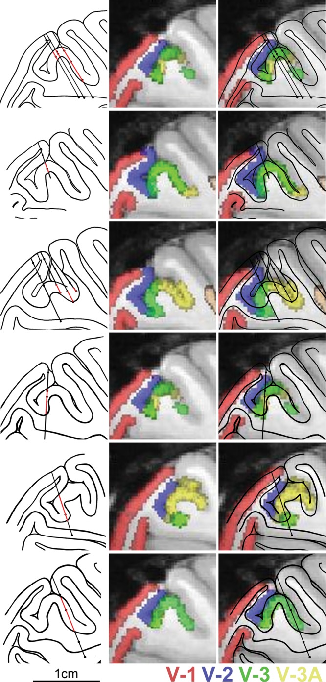
Reconstruction of the visual areas traversed during 6 experiments (each row from one experiment). Left panels show tracings of the sagittal sections containing the electrode tracts. Regions along the electrode penetration in red are those in which disparity-tuned neurons were identified. Center panels show the matching slice from a monkey atlas of visual areas generated with fMRI. Right panels, overlay.
Figure 5.

Quantification of single-cell results. (A) Proportion of neurons recorded in each visual area selective for binocular disparity. Error bars show upper and lower estimates as predicted from the alignment of the electrode penetrations with the MRI atlas of visual areas. Some electrode penetrations glanced the predicted border between V-3 and V-3A. The upper estimate includes all neurons that could potentially have resided within the visual area; the lower estimate includes only those neurons that were very likely to have resided in the visual area. (B) Population distribution of disparity preferences among extrastriate disparity-tuned neurons. (C) fMRI response to near- versus far-disparity stimuli. Near-disparity bias index was calculated as [(Response to drifting random dot stereograms containing only near disparities − Response to drifting random dot stereograms containing only far disparities)/(Response to drifting random dot stereograms containing only near disparities + Response to drifting random dot stereograms containing only far disparities)]. Asterisk shows a significant bias for near disparities, P < 0.05 (unpaired 2-tailed t-test, N = 4 hemispheres). CIPS: caudal intraparietal sulcus. (D) Tracing of the sagittal section containing the electrode penetration (see Fig. 3B) showing layer 4 (black line) and the base of the lunate sulcus (dashed line), an anatomical landmark that coincides with the border between V-2 and V-3. (E) The total number of disparity-tuned and nondisparity-tuned neurons within 1 mm bins at various distances from the base of the lunate sulcus (negative numbers are within putative V-2; positive numbers are within putative V-3/V-3A). (F) The proportion of neurons that showed disparity tuning recorded at various distances from the base of the lunate sulcus (compare with A).
The use of atlases to assign extrastriate borders assumes that there is little or no interanimal variability. This is assumption is not strictly valid. To provide an independent analysis of the location of the cells, we therefore calculated each cell's distance from the base of the lunate sulcus, an anatomical landmark that is often coincident with the border between V-2 and V-3. For cells close to layer 4, this distance was calculated by tracing along layer 4 to the base of the lunate (Fig. 5D). For cells outside of layer 4, we projected the location of the neuron onto layer 4 using a line perpendicular to the cortical sheet that passed through the neuron. Figure 5E shows the raw number of disparity-tuned and nondisparity-tuned cells recorded at each distance from the base of the lunate (1 mm bins). To compare with Figure 5A, Figure 5F shows the percentage of neurons that were disparity tuned, again as a function of the distance from the base of the lunate. We pooled cells on the left of “0” (i.e. cells up the bank of the lunate into V-2) and cells on the right of “0” (i.e. cells up the annectant gyrus into area V-3 or V-3A). We used a χ2 test to compare the proportion of stereo cells in likely V-2 (21%) with that in likely V-3/V-3A (43%). The difference is significant (χ2 statistic = 26.568, df = 1, P = 2.5 × 10⁻⁷).
Bias for Near Disparities
Figure 5B is a population histogram showing the number of neurons with various disparity preferences. The histogram shows a subtle bias for cells with near tuning preferences in V-2 (χ2 value 4.8, df = 1, P = 0.03) and V-3 (χ2 statistic = 17.065, df = 1, P = 0.00004). However, this bias was not present in V-3A (χ2 statistic = 2.283, 1 degree of freedom, P = 0.13). We tested the extent to which this bias is reflected in the fMRI responses, by comparing the responses to near-disparity checkerboards with those to far-disparity checkerboards, using a stimulus paradigm identical to that described in Tsao, Vanduffel, et al. (2003). The data confirm the findings of Tsao et al., showing a strong disparity bias in V-3A and the caudal intraparietal sulcus (CIPS; data not shown). All areas showed stronger responses to the near-disparity checkers, although among the areas from which single-unit recordings were obtained, the result was only significant in V-2 and V-3 (Fig. 5C). Interestingly, the strongest near bias in the fMRI experiment was obtained in area V-4, an area from which Hubel and Wiesel did not record.
A plot of the receptive-field maps of sequential neurons suggests a topographic representation and provides a clue that the neurons along the penetration shown in Figure 3 were not in the same visual area (Fig. 6). The receptive fields of neurons 1–19 clustered along the vertical meridian representation, consistent with their physical location near the border of V-1 and V-2; neurons 20–42 shifted progressively away from the vertical meridian into the lower left visual quadrant, consistent with the retinotopic representation in V-2. The receptive fields of neurons 44–49, meanwhile, were larger and found at more peripheral locations. (Supplementary Figures 3 and 4 show the receptive field reconstructions for 7 additional penetrations spanning V-2, V-3, and V-3A.) This difference in receptive field size cannot be attributed simply to a more peripheral visual field representation. Figure 7 shows that neurons assigned to V-3/V-3A tended to have larger receptive fields at any given eccentricity than those in V-2 (analysis of covariance, Tukey's multiple comparison test, α = 0.05). There is also a trend, albeit insignificant, for V-3A neurons to have larger receptive fields than V-3 neurons.
Figure 6.

Reconstruction of the receptive-field maps for all the neurons encountered on the experiment conducted on 24 June 1969 (see Figs 2 and 3). “S” indicates disparity-tuned (“stereo”) neurons. The horizontal tick marks along the vertical line show the center of gaze. The receptive fields have been splayed out along the vertical axis, so that individual overlapping receptive fields can be easily discriminated. See also Supplementary Figures 3 and 4.
Figure 7.

Receptive field width as a function of the eccentricity of the receptive field within the visual field for neurons recorded in V-2, V-3, and V-3A.
Bias for Vertical Orientation Tuning
Measurements of the orientation preference were made for most recorded neurons. Figure 8 shows a smoothed population histogram of orientation preferences for disparity-tuned cells (black lines) compared with nondisparity-tuned cells. The majority of disparity-tuned neurons preferred vertically oriented bars (or bars with a strong vertical component) as indicated in the figures by the peak toward 0°. Supplementary Figure 5 is the original figure prepared around 1970, showing the results for each cell separately: Each dot along the perimeter of the semicircle indicates a single cell with a tuning preference at the corresponding angle (bias for vertical orientations, Supplementary Figure 5A, χ2 value 54, df = 17, P = 0.00001). The nondisparity-tuned neurons showed a more uniform distribution of orientation preferences (Supplementary Fig. 5B, χ2 value 6.8, 17 degrees of freedom, P = 0.9).
Figure 8.

Orientation preferences for the population of disparity-tuned (black lines) and nondisparity-tuned (gray lines) neurons in V-2, V-3, V-3A, and combined. Neurons selective for vertical bars are plotted at 0°. Supplementary Figure 5 shows results for each cell separately. Supplementary Movie 4 shows tests of the orientation sensitivity of one example neuron.
The population of neurons showed a continuous range of disparity-tuning preferences (Fig. 5). In the original analysis conducted around 1970, cells were categorized into 3 groups: Cells with tuning preferences for near, zero, or distant disparities (Supplementary Fig. 6). The results showed a remarkable feature of the disparity-tuned neurons: They tended to cluster according to disparity preference (Fig. 9, “N” for near; “D” for distance). We quantified this trend in Figure 9C. Clustering of neurons by disparity preference is evident by an elevated signal along the y = x diagonal. Although the cells were originally binned into only 3 categories, the clustering is consistent with a continuous map of disparity preferences (Fig. 9D), as described by others in macaque area MT (DeAngelis and Newsome 1999) and cat area 18 (Kara and Boyd 2009).
Figure 9.

Clustering of disparity-tuned neurons by disparity preference (N = near; 0 = zero; D = distant). (A) Tracing of the sagittal slice from an example experiment containing 4 penetrations. Area designations were obtained by aligning the slice with an atlas of visual areas obtained with fMRI. (B) Receptive field reconstructions for neurons 18 through 27 recorded in the second penetration, marked by an arrowhead in (A). The horizontal tick marks along the vertical line show the center of gaze. The receptive fields have been splayed out along the vertical axis, so that individual overlapping receptive fields can be easily discriminated. For cells preferring distant disparity, the cell peaked with the left eye's receptive field (solid line) deviated to the right of the right eye's receptive field (dashed line); for cells preferring near disparity, the optimal stimulus configuration required the left eye's receptive field displaced to the left of the right eye's receptive field. (C) Quantification of spatial clustering by visual area using values binned as either “near,” “distant,” or “zero” disparity preference, as done in the original analysis from around 1970 (see Supplementary Fig. 6). Scale bar shows the number of cells. Spatial clustering is evident in peaks along the y = x axis. (D) Quantification of spatial clustering by visual area. Note that near-disparity preferences are plotted at plus values, following contemporary conventions. Spatial clustering is evident in peaks along the y = x axis. For panels (left to right), the R2 values are 0.77, 0.78, 0.23, and 0.51.
Finally, the results suggest that many disparity-tuned neurons were “obligate binocular,” more-or-less insensitive to stimulation of either eye alone (Fig. 2C; Supplementary Movies 2 and 5). Obligate binocular neurons have been described in V-2 (Ts'o et al. 2001) and inferior temporal cortex (Uka et al. 2000), but are rare in area MT (Maunsell and Van Essen 1983). Figure 10A, B show histograms quantifying the ocular dominance preferences and binocular interactions of disparity-tuned and nondisparity-tuned neurons. Values of “4” in these plots indicate neurons with roughly balanced responses to stimulation of either eye alone, whereas values 1 and 7 indicate unbalanced responses dominated by one or the other eye. The bar marked by an “X” shows the cells determined to be obligate binocular, which were not classified in the numerical scale because they could not be stimulated with either eye alone. The largest category of disparity-tuned neurons was obligate binocular cells.
Figure 10.

Responses to monocular versus binocular stimulation. (A) Population distribution of disparity-tuned neurons. Values of “1” correspond to neurons whose responses were entirely driven by the left eye; “7,” correspond to neurons whose responses were entirely driven by the right eye; and “4,” by both eyes equally. Obligate binocular cells, which require simultaneous stimulation of both eyes, are shown in column “X.” (B) Distribution of nondisparity-tuned neurons.
Discussion
The first description of neurons sensitive to binocular disparity in monkeys was made in a brief report in 1970 (Hubel and Wiesel 1970). Here, we give a fuller account of those experiments. The disparity-tuned neurons were often obligate binocular, requiring simultaneous stimulation of both eyes to elicit responses. This property shows that the neurons perform a nonlinear computation on the binocular inputs, consistent with a role in stereoscopic depth perception. The recordings were made in a region originally described as area 18. Aided by an atlas of visual areas, we now can be sure that some of these disparity-sensitive cells were indeed in V-2, the area now synonymous with area 18. These cells most likely resided within the thick darkly stained cytochrome-oxidase stripes (Hubel and Livingstone 1987; Ts'o et al. 2001). But many disparity-sensitive cells, especially those in the buried annectant gyrus, were almost certainly in V-3 or V-3A, regions that have since been shown to contain many disparity-tuned neurons (Felleman and Van Essen 1987; Poggio et al. 1988; Adams and Zeki 2001; Backus et al. 2001; Tsao, Vanduffel, et al. 2003; Neri et al. 2004; Ponce et al. 2008; Anzai et al. 2011). The delay in the full description of these results was due to the realization that the large expanse of cortex from which recordings were made was most likely comprised of more than one area (Hubel and Wiesel 2005).
Using stringent albeit subjective criteria to define a neuron as coding for disparity, 22% of V-2 cells and 42% of V-3/V-3A cells were disparity-tuned. In comparison, Poggio et al. (1988) found that as many as 80% of neurons in V-3/V-3A were disparity-tuned, although the criterion they used to assess disparity tuning was probably more liberal than that used by other groups. In a large quantitative study, Anzai et al. report that 56% of V-3 cells and 53% of V-3A cells were disparity tuned. These fractions are comparable with those reported by 2 other studies (Felleman and Van Essen 1987; Adams and Zeki 2001), but are slightly higher than those obtained presently. This discrepancy might be attributed to the more sensitive criteria for determining disparity sensitivity made available by quantitative methods. Hubel and Wiesel's general cautiousness for assigning a functional specialization might also account for their oversight regarding disparity tuning of V-1 cells: V-1 cells with disparity tuning tend to have smaller disparity-tuning preferences than disparity-tuned neurons in extrastriate regions. Contemporary consensus is that about half of V-3 and V-3A neurons are selective for stereo cues.
Are V-3/V-3A Specialized for Stereopsis?
Hubel and Wiesel did not find disparity tuning among V-1 neurons, which prompted their exploration of extrastriate neurons. Disparity-tuned neurons within V-2 have since been shown to be clustered (Hubel and Livingstone 1987), and V-2 appears to play a greater role than V-1 in encoding retinal disparities (Bakin et al. 2000; Ts'o et al. 2001; Thomas et al. 2002). Other investigators have focused attention on V-3/V-3A (Anzai et al. 2011), and some have concluded that these areas are specialized for stereoscopic depth (Adams and Zeki 2001). In support of this idea, the proportion of disparity-tuned neurons in V-3/V-3A was higher than the proportion in V-2, a finding confirming the trends observed by Poggio et al. (1988). But other single-unit studies have found roughly the same proportion of disparity-tuned neurons in V-2 and V-3/V-3A (Anzai et al. 2011). It is not clear what accounts for the discrepancy between these different single-unit studies. A specialization for stereopsis within V-3/V-3A is supported by the observation that the disparity-tuned neurons within these regions are clustered by disparity preference (Fig. 9). This finding confirms observations by 2 other groups (Adams and Zeki 2001; Anzai et al. 2011). But this attribute is not unique to V-3/V-3A: Cells in V-2 were also clustered by disparity preference (Fig. 9). Thus, we conclude that while the absolute numbers of disparity-tuned neurons may increase from V-2 to V-3/V-3A, all these areas appear to play an important role in encoding retinal disparities, and each area almost certainly contributes to encoding other aspects of the visual world.
A Near Bias
A near bias amongst neurons involved in computing stereopsis is predicted by psychophysics (Jansen et al. 2009). The single-unit recording experiments showed that the population of disparity-tuned cells was slightly biased for near disparities within areas V-2 and V-3, but not V-3A. This finding confirms the observations made by Adams and Zeki (2001). In a meta-analysis of single-unit experiments conducted in dorsal (V-3, V-3A, and MT) and ventral areas (V-4), Anzai et al. (2011) concluded that a near bias is more prominent in ventral areas. We tested this hypothesis with an fMRI experiment (Fig. 5C); the results support the hypothesis, revealing a striking asymmetry in the extent of the near bias within ventral visual areas. In fact, the near bias was only significant in V-2, V-3, and V-4, and not significant in V-3A, MT, and CIPS, consistent with the results of the single-unit physiology described presently. The single-unit recordings provide evidence for a near bias among disparity-tuned neurons in the visual system, but this bias appears to be more substantial in brain regions (e.g. area V4) from which single-unit recordings were not made.
A Preference for Vertical Orientations
Models of disparity selectivity typically generate maximal output for disparities that are orthogonal to the preferred orientation (Ohzawa et al. 1990; Qian 1994; Fleet et al. 1996). This is a consequence of a hierarchical algorithm in which the orientation tuning is generated by an initial linear stage and the disparity selectivity is generated subsequently (Read and Cumming 2004). The finding that the neurons with obliquely oriented fields showed some vertical disparity tuning is consistent with these models. In the most well-documented cases, the disparity tuning was broadest along the orientation axis, as has been shown for disparity-tuned neurons in cat (Sasaki et al. 2010). The stimulus used to assess disparity was typically an oriented bar. This stimulus is not isotropic, which complicates the interpretation of the results: An oblique bar presented with only a vertical displacement to each eye will also have correspondence between the 2 eye inputs along the horizontal axis (the “correspondence problem”), although not to matching locations along the bar. Thus the conclusions regarding the contribution of the extrastriate neurons to computing vertical disparity are tentative. Indeed, subsequent measurements of vertical disparity tuning in monkey V-1 neurons using random dot stereograms (which are isotropic) have called into question the assumption that maximal disparity sensitivity is orthogonal to orientation tuning (Cumming 2002).
Because the eyes are horizontally displaced, most binocular disparity information available to an observer is along the horizontal axis; moreover, disparity signals in natural scenes are strongly biased along the horizontal axis (Read and Cumming 2004). Presumably, a system that is well adapted to encode behaviorally relevant disparities would be biased toward encoding horizontal disparities. Such an adaptation could be achieved either if disparity computations were performed independent of orientation computations (Cumming 2002), and/or if the population of neurons contributing to disparity calculations were biased for vertical orientation preferences. Consistent with this latter prediction, we report an over-representation of vertically orientation-tuned neurons and an under-representation of horizontally orientation-tuned neurons among disparity-selective cells when compared with nondisparity-selective cells (Fig. 8).
Summary
In summary, the classic single-unit recording experiments described here show that disparity-tuned cells in extrastriate cortex are located not only in V-2, as implied by the original description of these experiments, but also in V-3 and V-3A. The results confirm several important features of disparity-tuned neurons described in the years since these experiments were performed: that the cells often required stimulation of both eyes to elicit responses (providing evidence for functional specialization); were biased for near disparities (a neural correlate of a psychophysical bias); tended to prefer vertical orientations (as predicted by computational models); and clustered by disparity preference (extending columnar organization to a new domain). Although these experiments were initially described only in a brief report, they were widely discussed and have been extensively elaborated in the years since they were conducted. It is reassuring to observe that the main conclusions from this work are consistent with those derived using considerably more sophisticated and quantitative methods.
Experimental Procedures
Electrophysiological Experiments
Overview
All microelectrode experiments were conducted between 9 April 1968 and 17 March 1970, performed by Hubel and Wiesel at Harvard Medical School with procedures approved by the animal use committee at the time. When referring to performing single-unit recording experiments, the “we” refers to David Hubel and Torsten Wiesel. In their 1970 paper, Hubel and Wiesel reported on recordings from 627 cells. Our contemporary analysis of the original experimental records has enabled us to recover information for 626 cells; 272 were originally reported as somewhat responsive to binocular depth cues (272 of 626, 43%). A smaller subset (206) was later classified as depth cells according to stricter criteria requiring excitatory responses and clearly peaked disparity-tuning curves (e.g. Fig. 2). Cells peaking at zero disparity were required to have marked excitation with eyes in register so as to distinguish them from cells that were purely binocular and not tuned to disparity (see Supplementary Fig. 1 for an example of a binocular neuron lacking disparity tuning). Of these 206 cells, we have been able to recover detailed information about 203 cells. The present report documents the putative area locations of 177 of these 203 cells and their disparity tuning along the near-far axis (see Fig. 5); the histological sections for three experiments were missing, precluding area assignments. Hubel and Wiesel were able to resolve orientation tuning for 44 disparity-tuned and 134 nondisparity-tuned cells in V-2, 26 disparity-tuned and 54 nondisparity-tuned cells in V-3, and 87 disparity-tuned and 84 nondisparity-tuned cells in V-3A (Fig. 8A,B). The columnar organization of the disparity-tuned cells reported in Figure 5 is evaluated in Figure 9. Hubel and Wiesel were able to resolve ocular dominance indices for 45 disparity-tuned and 158 nondisparity-tuned cells in V-2, 14 disparity-tuned and 38 nondisparity-tuned cells in V-3, and 72 disparity-tuned and 55 nondisparity-tuned cells in V-3A (Fig. 10).
The number of neurons recorded does not include cells recorded prior to the time that disparity-tuned cells were recognized. About 90% of penetrations were made in the sagittal plane, usually with the electrode angled forward so as to enter the occipital lobe normal to the surface, as nearly as possible. For histological confirmation of penetrations, brains were usually sectioned in the sagittal plane. In this plane, it is much easier to interpret sections of the rather complex lunate sulcus, which contains most of extrastriate cortex that was explored. As described in the section fMRI Methods, the use of a stereotaxic reference frame facilitated comparison of the histological sections with a functional atlas.
Surgical Procedures for Single-Unit Electrophysiology
Details of the surgical procedures are published elsewhere (Wiesel and Hubel 1966; Hubel and Wiesel 1968). Animals were anesthetized with intraperitoneal sodium pentothal (35 mg/kg), and additional doses of the drug were given at half-hour intervals. The eyes were paralyzed with a combination of curare and gallamine triethiodide (2–3 mg/kg) given intramuscularly at half-hour intervals. The animals' condition was followed closely by observing body temperature, since a steady decline in temperature usually meant an early end to an experiment. In some animals, the cells outside of area 17 seemed much more vulnerable than those in 17, the first signs of failing being a marked increase in background activity and loss of stimulus specificity, so that for example, a slit in any orientation moved in any direction, or even a small spot, evoked brisk responses. When this happened the experiment was usually terminated at once, and for the sake of the health and sanity of the scientists, no experiments were prolonged beyond 19 h.
Visual Stimuli for Single-Unit Electrophysiology
Visual stimulation was by the usual projection method of Hubel and Wiesel (1959, 1962), modified in several ways for detailed binocular studies. The animal's head was held in a Horsley-Clarke apparatus, the eyes held open and protected with contact lenses filled to obtain focus of objects placed at the screen 1.5 m away (Fig. 1). Focus was checked with a streak retinoscope (Copeland). Position on the screen corresponding to the retinal disks and foveas were determined by the projection method (Hubel and Wiesel 1959). The direction of gaze of the left eye was adjusted with a variable (Risley) prism. By rotating the prism in its housing and varying its setting, the visual axis could be deviated up to 30° in any direction. To monitor this direction, we found it convenient to shine a narrow beam of light from the side, through a 45° mirror and out through the prism onto the screen. The monitor spot, about 1 min of arc, indicated the relative prism setting, which could be measured directly in degrees (at 1.5 m, 1in. = 1°).
Recordings were made with tungsten microelectrodes inserted hydraulically through a 2-mm hole in the skull and dura, in a system sealed off from the atmosphere. Because eye position is crucial for studies of binocular interaction, and since over many hours there were inevitably some eye movements, we found it necessary to check eye position each time a receptive field was mapped. To do this we mounted a separate tag electrode into area 17, choosing a region in 17 in which the cells' receptive fields would be as close as possible to the fields we were studying in extrastriate cortex. Thus for areas close to the macula, we generally placed the tag electrode laterally in 17 of the other hemisphere close to the fovea representation. A suitable tag cell in 17 was one that could be strongly driven with either eye; this cell was then held as long as possible, usually for many hours. After studying a cell in extrastriate cortex with the “business” electrode, the tag-cell receptive field was immediately checked in both eyes to see if either eye had moved, as would be indicated by a shift in the relative position of the tag-cell receptive field measured separately in the 2 eyes. In this way, it was possible to keep track of eye position for long periods. This method allowed us to detect disparities in relative position of receptive fields in 2 eyes to approximately 4 min of arc. This precision was not obtainable with the method of projecting the foveas, and in many cases, it was far more convenient and rapid.
For most tests of extrastriate neurons in the present report, the stimulus was a stationary or moving spot or line (slit, edge, or dark bar) projected on the screen with a hand-held slide projector. Stimuli had a light-dark ratio of 1–1.5 log units, dark areas having peak intensity of about 1 log cd/m2. In some of the later experiments, stimuli were generated with a special purpose computer on a large television screen at 1.5 m distance. This method provided similar results, but was more cumbersome. For the various stimuli (slits, dark bars, edges, and tongues), the size position, orientation, and rate and excursion of movement could all be adjusted continuously.
Responses and stimuli were documented using a mechanical typewriter (mitigating electrical noise during recordings). For some recordings, the neural responses were recorded on a videotape recorder (Sony EV 210), allowing subsequent quantitative plotting of the responses. The various tuning curves presented in this manuscript were obtained by digitizing and analyzing these records. In each microelectrode penetration, several lesions were made by passing current, usually 2 μA for 2 s (electrode negative). The formalin and gluteraldehyde-fixed brain was subsequently serially sectioned and Nissl stained.
Functional Magnetic Resonance Imaging
Overview
To conduct the fMRI experiments, alert animals were rewarded for maintaining fixation during a “meridian-mapping” experiment in which visual stimulation with black-and-white flickering checkers was restricted to wedges along the vertical meridian for a given period of time and then along the horizontal meridian (repeated many times). Area boundaries were defined as the regions showing greater responses to stimulation along the horizontal or vertical meridians; for example, the border between V-1 and V-2 would be indicated by a peak in the response to vertical meridian stimulation. We also obtained high resolution anatomical MR scans of the same animals. An undergraduate student and a technician with initially no knowledge on the purpose of the experiment selected from the anatomical MR images of the 4 hemispheres the sagittal slice (0.35 mm thick) that best matched each histological section from the Hubel and Wiesel experiments. These best-matches were confirmed by an experienced neuroanatomist, Vladimir Berezovskii, using the stereotyped location of the boundary between V-1 and V-2 as a fiduciary landmark. Area designations obtained from the fMRI experiments were then projected onto the anatomical MR slices, and the likely area locations of the recorded cells were identified (e.g. Figs 3 and 4).
Procedures for conducting fMRI in alert monkeys are given elsewhere (Conway et al. 2007). As previously described (Lafer-Sousa et al. 2012), 2 male rhesus macaques (7–8 kg) were scanned at Massachusetts General Hospital Martinos Imaging Center (MGH) in a 3-T Allegra with AC88 insert (Siemens, New York, NY, USA) scanner using a custom-made 4-channel send/ receive surface coil and standard echo planar imaging (repetition time = 2 s, 98 × 63 × 98 matrix, 1 mm3 voxels). Using positive reinforcement, animals were trained to sit in a sphinx position in a plastic chair placed inside the bore of the scanner and to fixate a central spot presented on a display screen 49 cm away. The head position was maintained using surgically implanted custom-made plastic head posts (surgical procedures described in Conway et al. 2007; Lafer-Sousa et al. 2012). An infrared eye tracker (ISCAN, Burlington, MA, USA) was used to monitor eye movements, and animals were only rewarded for maintaining their gaze within approximately 1° of the central fixation target. MR signal contrast was enhanced using a microparticular iron oxide agent (MION), Feraheme (AMAG Pharmaceuticals, Cambridge, MA, USA), injected intravenously into the femoral vein below the knee just prior to scanning (8–10 mg/kg, diluted in saline). Decreases in MION signals correspond to increases in blood-oxygen level-dependent (BOLD) response. All imaging and surgical procedures conformed to the local and National Institutes of Health guidelines and were approved by the Institutional Animal Care and Use Committees at Harvard Medical School and Wellesley College.
Visual Stimuli for fMRI Experiments
Visual stimuli were displayed on a screen (41° × 31°) 49 cm in front of the animal using a JVC DLA projector (1024 × 768 pixels). All stimuli spanned the entire screen, contained a small central fixation cross to engage fixation, and were presented in a blocked paradigm. Retinotopic mapping to determine area borders was done by presenting vertically and horizontally oriented achromatic checkered wedges that flickered in phase every 1 s. Responses to these wedges were used to determine the vertical and horizontal meridians delineating retinotopic visual areas V-1, V-2, V-3, V-3A, V-4, and V-5/MT. The stimulus sequence consisted of 32 s of horizontal wedges (99% luminance contrast, occupying 30° visual angle), followed by 32 s of uniform neutral gray, followed by 32 s of vertical wedges (occupying 60° visual angle), followed by 32 s of neutral gray, and so on for a total of 4 presentations of horizontal wedges and 4 presentations of vertical wedges. The significance maps comparing fMRI responses with horizontal and vertical wedges were painted on inflated surfaces of each animal's brain and used to define area borders. In separate experiments using the same animals, the representation of the central 3° was determined using blocks of flickering achromatic checkerboards that were either restricted to a 3° disc centered on the fixation dot or to the peripheral visual field outside the central 3°. In other sessions, high-resolution anatomical scans (0.35 mm × 0.35 mm × 0.35 mm voxels) were obtained for each animal while it was lightly sedated. Area border assignments were verified by comparing the area boundaries projected on high-resolution anatomical MRIs of the 2 animals with standard macaque atlases (Lewis and Van Essen 2000; Paxinos et al. 2000). Where the V-3/V-3A border was not well matched (a border that is not well resolved in the literature), assignments relied more heavily on functional activation (retinotopy), but V-3A always included all tissue labeled as V-3A in the Lewis and Van Essen (2000) surface atlas. Area assignments are projected on the anatomical MRIs using a color key. Retinotopy was assessed from 8496 (3328 meridian mapper and 5168 center vs. periphery) (5088 [1280 meridian mapper and 3808 center vs. periphery]) functional volumes in M1 (M2) obtained during 2 (2) sessions.
Sensitivity to stereoscopic depth was assessed by presenting in 32-second block design full-field drifting (2.2 deg/s) random dot stereogram checkerboards. Blocks contained either near disparity checks (0–0.22°), far disparity checks (0–0.22°), or no disparity (zero disp.) replicating the experimental procedures of others (Tsao, Vanduffel, et al. 2003). Intervening blocks of uniform neutral gray were presented between stimulus blocks. Stimulation of each eye was achieved by the use of colored filters (red-cyan goggles). The dot density was 15%, and dot sizes were approximately 0.08° in diameter. The luminance of the red dots through the red filter was 20.36 cd/m2, and through the cyan filter was 3.64 cd/m2. The luminance of the cyan dots through the cyan filter was 23.98 cd/m2, and through the red filter was 1.38 cd/m2. Stereo-sensitivity was assessed from 4784 (5408) functional volumes in M1 (M2) obtained during 1 (1) session.
Data analysis was performed using the FREESURFER and FS-FAST software (http://surfer.nmr.mgh.harvard.edu/) and custom-written Matlab scripts. The surfaces of the high-resolution volumes were reconstructed and inflated using FREESURFER; functional data were registered to each animal's own anatomical volume using the JIP toolkit (provided by Joseph Mandeville). Data were motion corrected with the AFNI motion correction algorithm (Cox and Hyde 1997) and were intensity normalized. Spatial smoothing was applied to the inflated maps (full-width at half maximum 1.5 mm). More detailed analysis methods are given elsewhere (Conway and Tsao 2006; Conway et al. 2007; Lafer-Sousa et al. 2012).
Supplementary Material
Supplementary material can be found at: http://www.cercor.oxfordjournals.org/
Authors' Contributions
D.H.H. and T.W. performed all the single-unit recording experiments. R.L.S. and B.R.C. performed the fMRI experiments. E.M.Y., R.L.S., and B.R.C. aligned the histological sections with the fMRI atlas. D.H.H. and B.R.C. wrote the manuscript.
Funding
This work was supported by the US National Institutes of Health (D.H.H., T.W.; and EY023322, B.R.C.), by the Bell Telephone Research Laboratories Inc. (D.H.H. and T.W.), by the National Science Foundation (0918064, B.R.C.), and by a Brachmann-Hoffman grant from Wellesley College (B.R.C. and E.M.Y.). This MRI experiments were carried out at the Athinoula A. Martinos Center for Biomedical Imaging at the Massachusetts General Hospital, using resources provided by the Center for Functional Neuroimaging Technologies (P41EB015896) a P41 Biotechnology Resource Grant supported by the National Institute of Biomedical Imaging and Bioengineering (NIBIB), National Institutes of Health. This work also involved the use of instrumentation supported by the NIH Shared Instrumentation Grant Program and/or High-End Instrumentation Grant Program. (S10RR021110).
Supplementary Material
Notes
We thank Vladimir Berezovskii for assisting in aligning the histological sections with the functional atlas and Lawrence Sincich for suggesting the analysis shown in Figure 5D–F. Functional MRI data were analyzed using the jip toolbox generously provided by Joseph Mandeville (http://www.nitrc.org/projects/jip/), and analysis scripts compiled by Sebastian Moeller. Janet Wiitanen provided technical assistance for the original physiological experiments. We thank Fergus Campbell, who ran the Chi-squared statistical tests for the orientation bias of disparity-tuned neurons. We are grateful to Richard Born, Jeremy Wilmer, Lawrence Sincich, Doris Tsao, Margaret Livingstone, and John Maunsell for comments and discussion. Conflict of Interest: None declared.
References
- Adams DL, Zeki S. Functional organization of macaque V3 for stereoscopic depth. J Neurophysiol. 2001;86:2195–2203. doi: 10.1152/jn.2001.86.5.2195. [DOI] [PubMed] [Google Scholar]
- Anzai A, Chowdhury SA, DeAngelis GC. Coding of stereoscopic depth information in visual areas V3 and V3A. J Neurosci. 2011;31:10270–10282. doi: 10.1523/JNEUROSCI.5956-10.2011. [DOI] [PMC free article] [PubMed] [Google Scholar]
- Backus BT, Fleet DJ, Parker AJ, Heeger DJ. Human cortical activity correlates with stereoscopic depth perception. J Neurophysiol. 2001;86:2054–2068. doi: 10.1152/jn.2001.86.4.2054. [DOI] [PubMed] [Google Scholar]
- Bakin JS, Nakayama K, Gilbert CD. Visual responses in monkey areas V1 and V2 to three-dimensional surface configurations. J Neurosci. 2000;20:8188–8198. doi: 10.1523/JNEUROSCI.20-21-08188.2000. [DOI] [PMC free article] [PubMed] [Google Scholar]
- Barlow HB, Blakemore C, Pettigrew JD. The neural mechanism of binocular depth discrimination. J Physiol. 1967;193:327–342. doi: 10.1113/jphysiol.1967.sp008360. [DOI] [PMC free article] [PubMed] [Google Scholar]
- Bough EW. Stereoscopic vision in the macaque monkey: a behavioural demonstration. Nature. 1970;225:42–44. doi: 10.1038/225042a0. [DOI] [PubMed] [Google Scholar]
- Conway BR, Moeller S, Tsao DY. Specialized color modules in macaque extrastriate cortex. Neuron. 2007;56:560–573. doi: 10.1016/j.neuron.2007.10.008. [DOI] [PMC free article] [PubMed] [Google Scholar]
- Conway BR, Tsao DY. Color architecture in alert macaque cortex revealed by fMRI. Cereb Cortex. 2006;16:1604–1613. doi: 10.1093/cercor/bhj099. [DOI] [PMC free article] [PubMed] [Google Scholar]
- Cox RW, Hyde JS. Software tools for analysis and visualization of fMRI data. NMR Biomed. 1997;10:171–178. doi: 10.1002/(sici)1099-1492(199706/08)10:4/5<171::aid-nbm453>3.0.co;2-l. [DOI] [PubMed] [Google Scholar]
- Cumming BG. An unexpected specialization for horizontal disparity in primate primary visual cortex. Nature. 2002;418:633–636. doi: 10.1038/nature00909. [DOI] [PubMed] [Google Scholar]
- Cumming BG, DeAngelis GC. The physiology of stereopsis. Annu Rev Neurosci. 2001;24:203–238. doi: 10.1146/annurev.neuro.24.1.203. [DOI] [PubMed] [Google Scholar]
- Cumming BG, Parker AJ. Responses of primary visual cortical neurons to binocular disparity without depth perception. Nature. 1997;389:280–283. doi: 10.1038/38487. [DOI] [PubMed] [Google Scholar]
- DeAngelis GC, Newsome WT. Organization of disparity-selective neurons in macaque area MT. J Neurosci. 1999;19:1398–1415. doi: 10.1523/JNEUROSCI.19-04-01398.1999. [DOI] [PMC free article] [PubMed] [Google Scholar]
- Felleman DJ, Van Essen DC. Receptive field properties of neurons in area V3 of macaque monkey extrastriate cortex. J Neurophysiol. 1987;57:889–920. doi: 10.1152/jn.1987.57.4.889. [DOI] [PubMed] [Google Scholar]
- Fize D, Vanduffel W, Nelissen K, Denys K, Chef d'Hotel C, Faugeras O, Orban GA. The retinotopic organization of primate dorsal V4 and surrounding areas: a functional magnetic resonance imaging study in awake monkeys. J Neurosci. 2003;23:7395–7406. doi: 10.1523/JNEUROSCI.23-19-07395.2003. [DOI] [PMC free article] [PubMed] [Google Scholar]
- Fleet DJ, Wagner H, Heeger DJ. Neural encoding of binocular disparity: energy models, position shifts and phase shifts. Vision Res. 1996;36:1839–1857. doi: 10.1016/0042-6989(95)00313-4. [DOI] [PubMed] [Google Scholar]
- Fox R, Blake RR. Stereoscopic vision in the cat. Nature. 1971;233:55–56. doi: 10.1038/233055a0. [DOI] [PubMed] [Google Scholar]
- Hegdé J, Van Essen DC. Role of primate visual area V4 in the processing of 3-D shape characteristics defined by disparity. J Neurophysiol. 2005;94:2856–2866. doi: 10.1152/jn.00802.2004. [DOI] [PubMed] [Google Scholar]
- Hof PR, Morrison JH. Neurofilament protein defines regional patterns of cortical organization in the macaque monkey visual system: a quantitative immunohistochemical analysis. J Comp Neurol. 1995;352:161–186. doi: 10.1002/cne.903520202. [DOI] [PubMed] [Google Scholar]
- Howe PD, Livingstone MS. V1 partially solves the stereo aperture problem. Cereb Cortex. 2006;16:1332–1337. doi: 10.1093/cercor/bhj077. [DOI] [PMC free article] [PubMed] [Google Scholar]
- Hubel DH. Tungsten microelectrode for recording from single units. Science. 1957;125:549–550. doi: 10.1126/science.125.3247.549. [DOI] [PubMed] [Google Scholar]
- Hubel DH, Livingstone MS. Segregation of form, color, and stereopsis in primate area 18. J Neurosci. 1987;7:3378–3415. doi: 10.1523/JNEUROSCI.07-11-03378.1987. [DOI] [PMC free article] [PubMed] [Google Scholar]
- Hubel DH, Wiesel TN. Brain and visual perception: the story of a 25-year collaboration. New York, NY: Oxford University Press; 2005. [Google Scholar]
- Hubel DH, Wiesel TN. Receptive fields, binocular interaction and functional architecture in the cat's visual cortex. J Physiol. 1962;160:106–154. doi: 10.1113/jphysiol.1962.sp006837. [DOI] [PMC free article] [PubMed] [Google Scholar]
- Hubel DH, Wiesel TN. Receptive fields and functional architecture of monkey striate cortex. J Physiol. 1968;195:215–243. doi: 10.1113/jphysiol.1968.sp008455. [DOI] [PMC free article] [PubMed] [Google Scholar]
- Hubel DH, Wiesel TN. Receptive fields of single neurones in the cat's striate cortex. J Physiol. 1959;148:574–591. doi: 10.1113/jphysiol.1959.sp006308. [DOI] [PMC free article] [PubMed] [Google Scholar]
- Hubel DH, Wiesel TN. Stereoscopic vision in macaque monkey. Cells sensitive to binocular depth in area 18 of the macaque monkey cortex. Nature. 1970;225:41–42. doi: 10.1038/225041a0. [DOI] [PubMed] [Google Scholar]
- Jansen L, Onat S, König P. Influence of disparity on fixation and saccades in free viewing of natural scenes. J Vis. 2009;9:1–19. doi: 10.1167/9.1.29. [DOI] [PubMed] [Google Scholar]
- Kara P, Boyd JD. A micro-architecture for binocular disparity and ocular dominance in visual cortex. Nature. 2009;458:627–631. doi: 10.1038/nature07721. [DOI] [PMC free article] [PubMed] [Google Scholar]
- Lafer-Sousa R, Liu YO, Lafer-Sousa L, Wiest MC, Conway BR. Color tuning in alert macaque V1 assessed with fMRI and single-unit recording shows a bias toward daylight colors. J Opt Soc Am A Opt Image Sci Vis. 2012;29:657–670. doi: 10.1364/JOSAA.29.000657. [DOI] [PubMed] [Google Scholar]
- Lewis JW, Van Essen DC. Mapping of architectonic subdivisions in the macaque monkey, with emphasis on parieto-occipital cortex. J Comp Neurol. 2000;428:79–111. doi: 10.1002/1096-9861(20001204)428:1<79::aid-cne7>3.0.co;2-q. [DOI] [PubMed] [Google Scholar]
- Logothetis NK, Guggenberger H, Peled S, Pauls J. Functional imaging of the monkey brain. Nat Neurosci. 1999;2:555–562. doi: 10.1038/9210. [DOI] [PubMed] [Google Scholar]
- Maunsell JH, Van Essen DC. Functional properties of neurons in middle temporal visual area of the macaque monkey. II. Binocular interactions and sensitivity to binocular disparity. J Neurophysiol. 1983;49:1148–1167. doi: 10.1152/jn.1983.49.5.1148. [DOI] [PubMed] [Google Scholar]
- Neri P, Bridge H, Heeger DJ. Stereoscopic processing of absolute and relative disparity in human visual cortex. J Neurophysiol. 2004;92:1880–1891. doi: 10.1152/jn.01042.2003. [DOI] [PubMed] [Google Scholar]
- Ohzawa I, DeAngelis GC, Freeman RD. Stereoscopic depth discrimination in the visual cortex: neurons ideally suited as disparity detectors. Science. 1990;249:1037–1041. doi: 10.1126/science.2396096. [DOI] [PubMed] [Google Scholar]
- Paxinos G, Huang X-F, Toga AW. The rhesus monkey brain in stereotaxic coordinates. San Diego, CA: Academic Press; 2000. [Google Scholar]
- Pettigrew JD, Nikara T, Bishop PO. Binocular interaction on single units in cat striate cortex: simultaneous stimulation by single moving slit with receptive fields in correspondence. Exp Brain Res. 1968;6:391–410. doi: 10.1007/BF00233186. [DOI] [PubMed] [Google Scholar]
- Poggio GF, Fischer B. Binocular interaction and depth sensitivity in striate and prestriate cortex of behaving rhesus monkey. J Neurophysiol. 1977;40:1392–1405. doi: 10.1152/jn.1977.40.6.1392. [DOI] [PubMed] [Google Scholar]
- Poggio GF, Gonzalez F, Krause F. Stereoscopic mechanisms in monkey visual cortex: binocular correlation and disparity selectivity. J Neurosci. 1988;8:4531–4550. doi: 10.1523/JNEUROSCI.08-12-04531.1988. [DOI] [PMC free article] [PubMed] [Google Scholar]
- Ponce CR, Lomber SG, Born RT. Integrating motion and depth via parallel pathways. Nat Neurosci. 2008;11:216–223. doi: 10.1038/nn2039. [DOI] [PMC free article] [PubMed] [Google Scholar]
- Qian N. Computing stereo disparity and motion with known binocular cell properties. Neural Comput. 1994;6:390–404. [Google Scholar]
- Read JC, Cumming BG. Understanding the cortical specialization for horizontal disparity. Neural Comput. 2004;16:1983–2020. doi: 10.1162/0899766041732440. [DOI] [PMC free article] [PubMed] [Google Scholar]
- Sasaki KS, Tabuchi Y, Ohzawa I. Complex cells in the cat striate cortex have multiple disparity detectors in the three-dimensional binocular receptive fields. J Neurosci. 2010;30:13826–13837. doi: 10.1523/JNEUROSCI.1135-10.2010. [DOI] [PMC free article] [PubMed] [Google Scholar]
- Thomas OM, Cumming BG, Parker AJ. A specialization for relative disparity in V2. Nat Neurosci. 2002;5:472–478. doi: 10.1038/nn837. [DOI] [PubMed] [Google Scholar]
- Tsao DY, Conway BR, Livingstone MS. Receptive fields of disparity-tuned simple cells in macaque V1. Neuron. 2003;38:103–114. doi: 10.1016/s0896-6273(03)00150-8. [DOI] [PMC free article] [PubMed] [Google Scholar]
- Tsao DY, Vanduffel W, Sasaki Y, Fize D, Knutsen TA, Mandeville JB, Wald LL, Dale AM, Rosen BR, Van Essen DC, et al. Stereopsis activates V3A and caudal intraparietal areas in macaques and humans. Neuron. 2003;39:555–568. doi: 10.1016/s0896-6273(03)00459-8. [DOI] [PubMed] [Google Scholar]
- Ts'o DY, Roe AW, Gilbert CD. A hierarchy of the functional organization for color, form and disparity in primate visual area V2. Vision Res. 2001;41:1333–1349. doi: 10.1016/s0042-6989(01)00076-1. [DOI] [PubMed] [Google Scholar]
- Uka T, Tanaka H, Yoshiyama K, Kato M, Fujita I. Disparity selectivity of neurons in monkey inferior temporal cortex. J Neurophysiol. 2000;84:120–132. doi: 10.1152/jn.2000.84.1.120. [DOI] [PubMed] [Google Scholar]
- Ungerleider LG, Desimone R. Cortical connections of visual area MT in the macaque. J Comp Neurol. 1986;248:190–222. doi: 10.1002/cne.902480204. [DOI] [PubMed] [Google Scholar]
- Van Essen DC, Dierker DL. Surface-based and probabilistic atlases of primate cerebral cortex. Neuron. 2007;56:209–225. doi: 10.1016/j.neuron.2007.10.015. [DOI] [PubMed] [Google Scholar]
- Van Essen DC, Zeki SM. The topographic organization of rhesus monkey prestriate cortex. J Physiol. 1978;277:193–226. doi: 10.1113/jphysiol.1978.sp012269. [DOI] [PMC free article] [PubMed] [Google Scholar]
- Verhoef BE, Vogels R, Janssen P. Contribution of inferior temporal and posterior parietal activity to three-dimensional shape perception. Curr Biol. 2010;20:909–913. doi: 10.1016/j.cub.2010.03.058. [DOI] [PubMed] [Google Scholar]
- Wheatstone C. Contribution to the physiology of vision—part the first. On some remarkable and hitherto unobserved phenomena of binocular vision. Philos Trans R Soc Lond B Biol Sci. 1838;128:371–394. [Google Scholar]
- Wiesel TN, Hubel DH. Spatial and chromatic interactions in the lateral geniculate body of the rhesus monkey. J Neurophysiol. 1966;29:1115–1156. doi: 10.1152/jn.1966.29.6.1115. [DOI] [PubMed] [Google Scholar]
Associated Data
This section collects any data citations, data availability statements, or supplementary materials included in this article.