A single-molecule long-read survey of the human transcriptome

Abstract

Global RNA studies have become central to understanding biological processes, but methods such as microarrays and short-read sequencing are unable to describe an entire RNA molecule from 5′ to 3′ end. Here we use single-molecule long-read sequencing technology from Pacific Biosciences to sequence the polyadenylated RNA complement of a pooled set of 20 human organs and tissues without the need for fragmentation or amplification. We show that full-length RNA molecules of up to 1.5 kb can readily be monitored with little sequence loss at the 5′ ends. For longer RNA molecules more 5′ nucleotides are missing, but complete intron structures are often preserved. In total, we identify ~14,000 spliced GENCODE genes. High-confidence mappings are consistent with GENCODE annotations, but >10% of the alignments represent intron structures that were not previously annotated. As a group, transcripts mapping to unannotated regions have features of long, noncoding RNAs. Our results show the feasibility of deep sequencing full-length RNA from complex eukaryotic transcriptomes on a single-molecule level.

The human transcriptome is extremely complex, with >100,000 distinct transcripts presently described for ~20,000 proteincoding genes. Short-read RNA sequencing has become a powerful tool for the description of gene expression levels and individual splice junctions^1–7. However, it is difficult to identify full-length transcript isoforms using short reads. Thus, a complete understanding of all spliced RNAs within a transcriptome is not yet possible and can be inferred only from a patchwork of short fragments. Furthermore, multiple amplification steps during library preparation complicate the quantification of expression levels. Given sufficient material, amplification free sequencing of full-length cDNA molecules provides a more direct view of RNA molecules. The Pacific Biosciences (PacBio) sequencing platform⁸ shows no context-specific errors⁹ and is widely appreciated for producing long, albeit low-quality, reads. Previous approaches^10,11 have used high-accuracy short reads to correct errors in these long reads, thus producing high-quality, hybrid long reads. However, error correction can produce artifacts owing to alignment errors and such hybrid reads are not truly single-molecule reads. An alternative approach relies on the recently improved read-length and base-calling algorithms of the PacBio platform and the use of circular molecules. When read length exceeds the length of the cDNA template by at least twofold, each base pair is covered on both strands at least once and the multiple low-quality base calls can be used to derive a high-quality, single-molecule, circular-consensus (CCS) read. These CCS reads are generated de novo without alignment to a reference.

To investigate the potential of PacBio sequencing for analysis of complex transcriptomes, we generated 476,000 CCS reads from cDNA with an average length of 1 kb to investigate the isoform complement of a diverse pool of RNA samples representing 20 human tissues and organs. We demonstrate that the limiting factor for CCS read length is primarily the cDNA-template size, which is often <1.5 kb, rather than the read length of the PacBio platform (~7 kbp). The majority of CCS reads represent all introns of the original transcript, including most of the 5′ exons. Comparison with the high-quality GENCODE 15 annotation¹² of the human transcriptome revealed many unannotated transcripts and isoform structures within the CCS data set and provided a more comprehensive assessment of the true complexity of the transcriptome.

RESULTS

General properties of CCS reads in cDNA sequencing To identify as many transcript isoforms as possible, we prepared and pooled total RNA from 20 distinct organs and tissue types. Unfragmented cDNA libraries were synthesized from polyA+ RNA using an anchored oligo-dT primer, and single-molecule long-read sequencing was performed using a real-time sequencer from Pacific Biosciences. We processed the resulting raw ‘continuous long reads’ using PacBio software, which yielded reads in two formats: high accuracy CCS reads and lower-accuracy sub-reads that result when the template has not been sequenced sufficiently to produce a CCS read¹³. After excluding short reads (<300 bp in length), we obtained a total of 476,000 CCS reads representing 476 million bases, and 5.1 million reads (4.7 billion bases) when all sub-reads were considered. We recently produced two long-read sequencing data sets using the 454 platform¹⁴. Although the 454 reads average 522 bp and offer many advantages, they usually do not cover entire RNA molecules. GENCODE version 15–annotated transcripts averaged 1,574 bp and most were no longer than 1–1.5 kb, although some transcripts were much longer. Comparing GENCODE transcript lengths to those of CCS reads revealed strong concordance, indicating that the latter were often full-length sequences up to ~2 kb (Fig. 1a). CCS read length is bounded by the length of the original continuous long reads, butalso by the length of the cDNA. To assess which of these two limiting factors is more important, we calculated for each CCS read the ratio of the length of the continuous long read to the length of the CCS read. For the vast majority, this ratio was between 5 and 15 (Fig. 1b), indicating that the original continuous long read typically covered the cDNA molecule many times and that most cDNAs are short enough to produce CCS reads. Moreover, CCS reads exhibited more constant quality values along the read than 454 reads (Fig. 1c).

Figure 1.

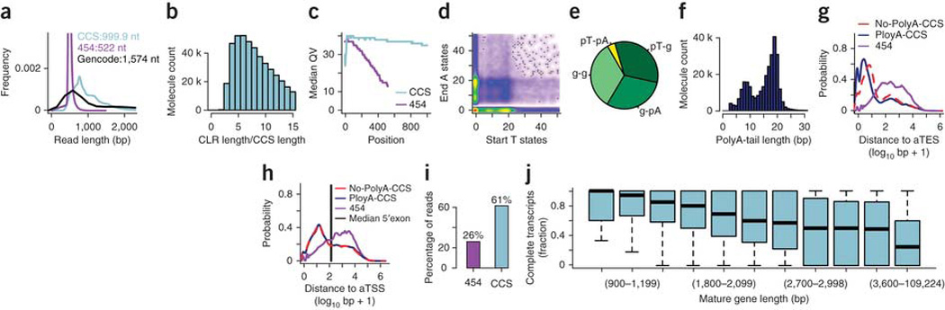
Completeness of cDNA molecules. (a) Length distribution of GENCODE-annotated transcripts, 454 reads and CCS reads. (b) Distribution of the ratio of the length of each CLR to the length of the CCS read derived from it. (c) Median quality values (QV) for 454 reads and CCS reads as a function of position in the read. (d) HMM polyA calling. Scatterplot of number of nucleotides in polyT state at the beginning of each read (x axis) and number of nucleotides in polyA state at the end of each read (y axis). Color-scale from white (absence of reads) to red (strong enrichment of reads). (e) Pie chart of reads showing four different categories, as defined in the text: g-pA, pT-g, pT-pA and g-g. The first three categories represent polyadenylated molecules, whereas the last category represents molecules lacking a polyA-tail. (f) Length distribution of polyA tails as determined by the HMM, with 19 nt being observed most often. (g) Distribution of distances from the 3′ ends of mappings to annotated transcript end sites (aTES) for polyadenylated molecules, nonpolyadenylated molecules and fragmented RNAs sequenced on a 454 instrument. (h) Distribution of distances from the 5′ ends of mappings to annotated TSS (aTSS) for polyadenylated molecules, nonpolyadenylated molecules and for fragmented RNAs sequenced on a 454 instrument. The black horizontal line represents the median length of 5′ exons of spliced transcripts. (i) Percentage of reads that meet two criteria: (i) the first splice site of the read is the first splice site of an annotated transcript and (ii) the last splice site of the read is the last splice site of an annotated transcript in GENCODE. The observed difference between 454 and CCS reads is statistically significant (two-sided Fisher test, P < 2.2e-16). (j) After calculating the percentage for CCS reads in i for each gene separately, we binned genes by the length of their longest annotated transcript. The plot shows boxplots for ten regularly-spaced bins (from 600–899 bp up to 3,300–3,599 bp) and one bin containing all longer genes. Note that the boundaries of the bins are only shown for every third bin.

We also determined whether cDNAs corresponded to full-length RNAs by evaluating their completeness at the 5′ and 3′ ends. The 3′ end of mRNAs is indicated by polyA tails, and, in our assay, these appear either as a polyT or polyA sequence depending upon the orientation of the template. Reads with ≥80% T content in the first 20 bp were labeled “polyT-start” and those with ≥80% A content in the last 20 bp “polyA-end.” This approach showed considerable variation in polyA/T length (Supplementary Fig. 1a–d).

To deal with this and with the higher error rates of sub-reads, we used a Hidden Markov Model (HMM) to assign each nucleotide to one of three states: “polyT” (pT), “polyA” (pA) or “genic” (g). Three main classes of molecules were identified: (i) molecules that started with a large number of polyT states, (ii) ended with a large number of polyA states or (iii) did neither (Fig. 1d). Analysis of base-pair frequencies around gene-polyA and polyT-gene HMM transitions showed that this HMM pinpoints the borders of polyA tails (Supplementary Fig. 1c).

We next classified all molecules into four classes: (i) starting in “genic” and ending in “polyA” (g-pA), (ii) starting in “polyT” and ending in “genic” (pT-g), (iii) starting in “polyT” and ending in “polyA” (pT-pA), all of which represent polyadenylated RNA molecules, and (iv) starting in “genic” and ending in “genic” (g-g). Approximately 67% of reads corresponded to polyadenylated RNAs (classes 1–3) (Fig. 1e). The most frequent polyA-tail length was 19, but variation could be observed (Fig. 1f). Reads that did not generate a CCS read, but spanned the entire cDNA, (full-pass sub-reads) were of lower quality (data not shown), and similar in terms of polyA tails, but longer (average 1,669 bp) than CCS reads (Supplementary Fig. 2). These reads therefore correspond to long transcripts.

Mapping of CCS reads and full-pass sub-reads to hg19 The 476,000 CCS reads were mapped against the hg19 genome using GMAP¹⁵, and analyzed as described previously¹⁴. This process does not rely on existing annotations of gene structures and therefore is relatively unbiased. GMAP identified one or more mappings for 98.8% of all CCS reads (Supplementary Fig. 3a). Supplementary Figure 3b shows the number of mappings to each chromosome, including multiple mappings for single molecules. For 84.6% of all mapped molecules, we found a single high-confidence mapping that covered a large portion of the cDNA molecule and scored higher than any other mappings¹⁴. As expected, few mappings (<4%) overlapped GENCODE12-annotated ribosomal RNA genes, which are not polyadenylated (Supplementary Fig. 3c). Of the high-confidence mappings (Supplementary Fig. 3d), about 6% fell into regions without a GENCODE-annotated transcript and 8% fell within introns (Supplementary Fig. 3e), possibly representing uncharacterized genes or, in the latter case, perhaps products of intron decay. Twenty nine percent fell entirely within regions containing a single exon.

Only a few sequences (<3%) potentially retained introns or parts of pre-mRNAs (Supplementary Fig. 3f) and the lengths of introns in mapped CCS reads rarely fell below 70 bp (Supplementary Fig. 3g), consistent with annotated introns¹⁴.

Comparison of 3′ mapping ends to annotated transcript ends We further assessed the 3′ completeness of the cDNA molecules by comparing the 3′ ends of mappings of spliced CCS reads to annotated transcript end sites (Fig. 1f) of the gene to which the CCS read was attributed. For all CCS reads, the median distance to the closest annotated transcript end sites was 6 bp (Fig. 1g). This contrasts to a median distance of 281 bp for fragmented and amplified material that we sequenced¹⁴ using the 454 platform. The median distance to the nearest annotated transcript end sites was 5 bp for polyadenylated CCS reads and 11 bp for nonpolyadenylated CCS reads (two-sided Wilcoxonrank-sum-test, P < 2.2e-16). Hence, polyadenylated CCS reads showed less sequence loss at their 3′ ends than did nonpolyadenylated CCS reads, although the 3′ ends of both were in strong agreement with annotated transcriptional end sites (Fig. 1g).

Comparison of 5′ mapping ends to annotated transcript start sites A similar analysis for 5′ ends found a median distance to the nearest annotated transcription start site (TSS) of 47 bp. This is short in comparison to our previously published 454 data (626 bp, Fig. 1h). More importantly, the median length of 5′ exons of annotated spliced transcripts (148 bp, mean = 237) lies between the two numbers above. This suggests that our sequenced cDNA molecules often contain all of the internal exons of a transcript and at least a portion of the 5′ exon. We found no appreciable difference between polyadenylated and nonpolyadenylated CCS reads (Fig. 1h). Therefore, CCS reads lacking a polyA tail may have lost some sequence after cDNA synthesis, perhaps during the end-repair step of library preparation. To assess whether CCS reads represented all of the splice sites of the transcript, we determined whether (i) the first mapped splice site of a read corresponds to the first splice site of an annotated transcript and (ii) the last mapped splice site of the read was the last splice site of the transcript. This occurred for 61% of all CCS reads and for 26% of all 454 reads (Fig. 1i). Note that this measurement of completeness would classify CCS reads with unannotated 5′ or 3′ exons as incomplete. We defined the completeness fraction on a gene-by-gene basis to determine the longest gene length for which a CCS read can represent the entire splice structure of an RNA molecule. We binned genes into 300-bp bins according to the length of the longest annotated mature transcript of the gene (that is, excluding intron length). For genes up to 1.2 kb, the fraction of complete transcripts was generally >0.9, and it stayed well above 0.5, up to 2.4 kb, after which lower values were observed (Fig. 1j). It is important to note that a gene may have transcripts considerably shorter than its longest one and different binning strategies may alter completeness fraction distribution for some bins.

The lower numbers of CCS reads per gene (relative to short-read sequencing) makes it more feasible to visually inspect all mappings for many genes. For example, we performed detailed manual analysis of relatively complicated candidate genes having exactly 12 exons in 4 kb of genomic space. GENCODE contains four such genes, and for three (AUP1, ACD and GPAA1) we found many full-length spliced CCS reads. The AUP1 gene had 27 aligned molecules, of which 26 were complete at the 3′ end, and 16 clearly represented the entire intron structure, reaching from the first exon to the last (Fig. 2a). The remaining 11 molecules represented previously unannotated TSS or incomplete cDNAs. For ACD, all six molecules represented its entire intron structure (Supplementary Fig. 4). For GPAA1, however, which has many different TSS, the transcripts appeared less complete, likely owing to incomplete cDNA synthesis or to unannotated 5′ exons or TSS (Supplementary Fig. 5).

Figure 2.

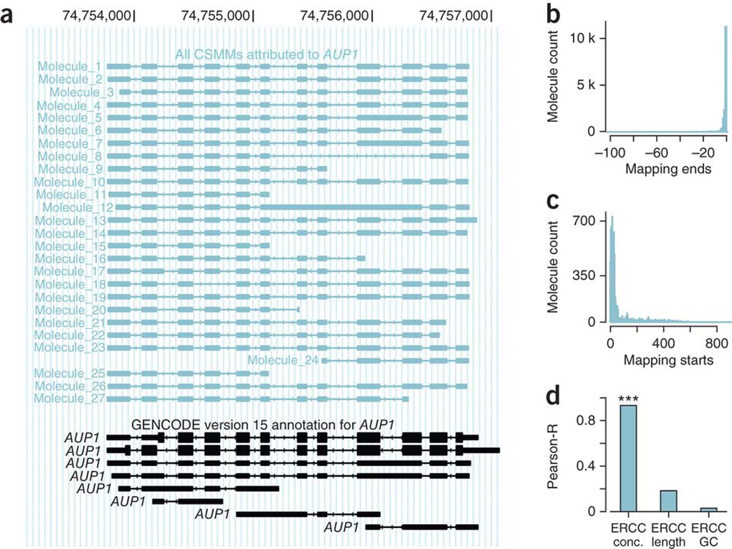
Assessment of completeness of CCS reads in controlled environments. (a) All CSMMs (blue) mapping to AUP1 (annotation in black). The only criteria that led to the choice of this example gene were: (i) its most exon–rich transcript had 12 exons and (ii) the genomic distance between gene start and the gene end was ≤4 kb (allowing easy display). (b) Distribution of missing 3′ nucleotides in CCS reads mapped to the original ERCC sequences. (c) Distribution of missing 5′ nucleotides in CCS reads mapped to the original ERCC sequences. (d) Pearson correlation between log-transformed number of CCS reads and log-transformed known ERCC concentration (left), log-transformed ERCC-sequence length (middle) and log transformed GC content of the ERCC sequences.

***P < 0.001 (Pearson correlation t-test – see cor.test in R (ref. ¹⁶)).

Sequence loss and expression of the ERCC control RNA To further assess the completeness of the cDNA molecules, we used the External RNA Control Consortium (ERCC)’s mixture of 92 distinct RNAs with known sequence and concentrations as a control. We sequenced two SMRT cells, and mapped the resulting 17,000 CCS reads against the original ERCC sequences, excluding the polyA tails. On the 3′ end, 75% of the mappings did not miss any nucleotides (Fig. 2b). On the 5′ end, the median number of missing nucleotides was 23 (out of the ~970 bp of the ERCC sequences, Fig. 2c) and 25 when considering ERCC sequences ≥1 kb. For CCS reads aligned to ERCC sequences ≥1.5 kb, however, a median of 377 nucleotides were missing. Because a CCS read represents the entire cDNA molecule, the missing nucleotides are a consequence of incomplete cDNAs. The Pearson correlation between the log-transformed number of CCS reads that mapped to each ERCC sequence and log-transformed known concentration of that sequence was 0.93 (P < 2.2e-16, Pearson correlation t-test; see cor.test in R (ref. ¹⁶)). The correlations between the log-transformed number of CCS reads and log-transformed RNA length and GC content were both below 0.2 and nonsignificant (Fig. 2d). This suggests little bias for sequences up to 1.5–2 kb (the maximal length of the ERCC sequences). However, some of the RNAs were present at relatively low concentrations andhad few or no mappings (a single read mapped to a reference is not a trustworthy quantification).

Splicing and intron structures of single molecules We identified several classes of CCS read mappings consistent with different patterns: split mappings (44%); unsplit mappings that did not overlap any annotated gene (13%), which likely represent novel single-exon genes and/or DNA contamination; unsplit mappings with a 75% overlap to an annotated single-exon transcript (19%), representing known single-exon transcripts; mappings that did not fall into the above categories but overlapped a spliced transcript’s 3′ exon (16%); and mappings that overlapped other exons of spliced transcripts (8%). The last two classes may represent cases of partial cDNA molecules that did not span an intron or unannotated single exon transcripts (Fig. 3a). If the last two classes originate from spliced RNA molecules, then ~67% of all polyadenylated RNA molecules in the cell between 0.3 kb and 2 kb are spliced. In agreement with this observation, when estimating this number from short-read sequencing from the ENCODE project, we find a ratio of 65%.

Figure 3.

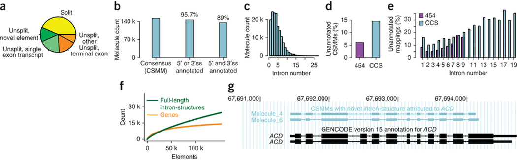
Exon-intron structure of molecules. (a) Pie-chart indicating the fraction of high confidence mappings that were: split into two or more segments (yellow); unsplit and overlapped no annotated element (darker green); unsplit with strong overlap with an annotated single-exon transcript (lighter green); unsplit with strong overlap of a terminal exon (darker orange); and unsplit overlapping other nonterminal exons (lighter orange). (b) Number of CSMMs having intron-consensus di-nucleotides at the ends of all splits (left), at least one split-end as an annotated splice site for all splits (middle) and only annotated splice sites (right). ss, splice sites. (c) Distribution of number of introns for CSMMs. (d) Percentage of unannotated CSMMs in 454 data¹⁴ and the CCS read data generated in this study. The observed difference is statistically significant (two-sided Fisher test, P < 2.2e-16). (e) Percentage of unannotated mappings for CSMMs with different numbers of introns for 454 and CCS read data. (f) Number of annotated genes (orange) and full-length isoforms (green), based on increasing numbers of CSMMs. (g) Example gene (ACD) with two unannotated isoforms shown by CSMMs. All CSMMs aligned to this gene are shown in Supplementary Figure 4.

The vast majority (92%) of split-mapped molecules had splice site–consensus nucleotides at every split-site in the molecule (consensus split-mapped molecule, CSMM). The GENCODE annotation has been considerably extended in the last few years, so that, for example, 95% of a set of short-RNA-seq introns¹⁷ can now be found in version 15. Most (96%) of CSMMs showed good agreement with GENCODE, as all of their introns had at least one annotated splice site and 89% of all CSMMs used only annotated splice sites (Fig. 3b). Approximately 69,400 CSMMs were identical in all of their splice sites to ~10,900 different GENCODE transcripts. CSMMs typically contained multiple introns and 9,000 contained ten or more introns. Even CSMMs with 20 or more introns exist (Fig. 3c). For aligned exonic blocks we found a median number of two mismatches per 100 bp, showing that these alignments are generally of high quality.

We represented each CSMM and each annotated transcript as the ordered list of its introns, that is, the position of each intron’s boundaries, (see ref. 14) and found that 14.5% of all CSMMs were not parts of annotated transcript structures. This percentage of candidates for unannotated transcript structures was higher than for 454, presumably owing to increased read length (Fig. 3d). The sum of the percentages (14.5% and 89%) exceeded 100%, because a transcript can represent an unannotated combination of known splice sites. This estimate is based purely on splice sites, and including TSS and polyA sites will increase the fraction of novel transcripts. Consistent with assessments of unannotated transcripts identified from 454 data, for CSMMs the percentage of unannotated intron structures increased with intron number. More unannotated transcripts were discovered from CCS reads, however, than from 454 data, regardless of intron number (Fig. 3e). This is likely due to the complexity of the sample and the lack of an amplification step in its preparation.

To estimate the false-positive rate for the classification of unannotated transcripts, we selected 10,000 random GENCODE transcripts and introduced errors into their sequences according to the error profile of CCS reads. We realigned these synthetic CCS reads to the hg19 genome and compared the resulting CSMMs to GENCODE, finding that 2.1% were classified as unannotated with respect to GENCODE (our false-positive rate). When querying longer gene structures (e.g., with lower quality sub-reads), one may find more unannotated isoforms, but alignments based on low-quality sub-reads also contain more false positives.

We next assessed the number of spliced GENCODE genes and fulllength isoforms identified as a function of sequencing depth. The number of genes began to saturate: the first 10 k CSMMs identified 4,408 distinct genes, but the last 10 k CSMMs, only 232, for a total of ~14,200. With the limitation that only full-length isoforms with known first and last splice sites can be classified as full length, we identified ~25,600 distinct full-length isoforms (Fig. 3f). Advanced modeling of molecular complexity¹⁸ suggested that increasing sequencing depth 20-fold should yield ~21,000 spliced GENCODE genes (95% confidence interval (CI; 15,497–29,868)) and ~139,000 full-length isoforms (95% CI (90,446 – 214,312)).

ACD is an example of a gene with a high fraction of unannotated isoforms (2/6) (see Supplementary Fig. 4 for all of its CSMMs). Both isoforms differ from the annotated gene structure in the skipping of an internal exon (Fig. 3g, right dashed box), and because both have this structure, it is less likely that these are instances of noisy splicing, which has been estimated to represent ~2% of the molecules for anaverage gene¹⁹. One of these transcripts alsocontains an unannotated alternative acceptor (Fig. 3g, left dashed box). The identification of different combinations of such novel elements highlights an advantage of long-read single molecule sequencing. That is, with higher sequencing depth, it should be possible to examine whether correlated distant splice sites²⁰ are used in the same or distinct molecules.

Detailed analysis of unannotated transcripts We noted that the distribution of unannotated spliced transcripts binned by number of introns (Fig. 3e) had multiple peaks, with oneintron transcripts being more likely to be unannotated than were two-intron transcripts. Therefore, we hypothesized that this distribution might be the mixture of multiple distributions. To investigate this, we assigned unannotated CSMMs to GENCODE genes when they shared at least one splice site, and recorded whether such an assignment was to a GENCODE protein-coding gene (79%), or to another spliced GENCODE gene-class—including long noncoding RNA genes (lncRNA) and pseudo-genes (“Other gene”, 8%), or whether no assignment could be made using splice site identity (“No gene,” 13%) (Fig. 4a). The lower read number for “Other genes” is consistent with the lower expression of lncRNAs²¹. This allowed us to compare the distributions of the categorized unannotated spliced transcripts that corresponded to different types of genes (Fig. 4b). Unannotated isoforms of genes encoding proteins usually contained multiple introns. CSMMs attributed to other genes also had multiple introns, albeit fewer than those attributed to genes encoding proteins. Alignments corresponding to no known gene mostly contained a single intron and rarely more than two.

Figure 4.

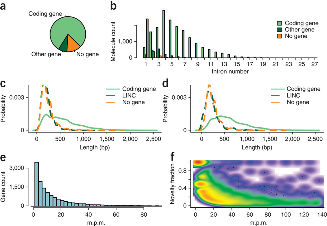
Analysis of unannotated transcripts. (a) Pie chart indicating the fraction of molecules corresponding to unannotated isoforms that shared a splice site with a known protein-coding gene (“coding gene”), with another spliced gene class (“other gene”) and those that do not share a splice site with any gene (“no gene”). (b) Same data as in a broken up by intron number in the CSMM mapping. (c) Proteincoding capacity of CSMMs. (d) Same plot as in c but showing the longest uninterrupted coding sequence starting with an ATG for each CSMM. (e) For known genes, we calculated the number of CSMMs that could be attributed to this gene (≥1 splice site in common) per million well-mapped reads (m.p.m.). (f) Scatterplot with m.p.m. on the x axis and the fraction of CSMMs that indicated an unannotated isoform of this gene on the y axis. Color scale from white (absence of molecules) to red (strong enrichment of molecules).

We then isolated CSMMs aligned to long intergenic non-coding RNAs (lincRNAs) from the “other gene” class and considered the three classes “Coding gene,” “lincRNA gene” and “No gene.” We used Geneid²² to find open reading frames (ORFs). ORFs for lincRNA genes were similar in size to ORFs for CSMMs that did not align to any annotated gene, whereas in many but not all cases CSMMs aligned to genes encoding proteins contained longer ORFs (Fig. 4c). A simple codon-counting approach gave similar results (Fig. 4d). About 5% of the CSMMs that were not assigned to a GENCODE gene (which have no splice sites in common with known genes) had Geneid ORFs much longer than the median of unannotated CSMMs and may harbor previously unreported peptide sequences. Using the number of molecules per million high-confidence mappings (m.p.m., Fig. 4e) as an expression value revealed an anti-correlation between expression and novelty, which can be simplified by the distinction of two classes of genes: a class of weakly expressed genes (within the collection of 20 tissues) with a majority of unannotated isoforms, an example of which is shown in Supplementary Figure 6, and a class of genes, many of which are expressed at higher levels, having unannotated minor isoforms (Fig. 4f). The latter are likely to be enriched for noisy splicing events, especially when the unannotated isoforms are of low frequency¹⁹.

DISCUSSION

In summary, we show four main points. First, one can monitor human RNA isoforms on a single-molecule level, without amplification or fragmentation. Second, the majority of sequenced cDNA molecules represent all splice sites of the original transcripts, although the success rate depends on the completeness of cDNA synthesis. For cDNAs up to 1.5 kb in length, this problem appears minor, and for those 2–2.5 kb, a large fraction of full-length reads are observed. Longer transcripts need to be interrogated using lower quality but longer sub-reads. Third, the molecules we sequence show the existence of unannotated splice isoforms. For high-quality CCS reads, 14.5% of the spliced mappings are different from known gene structures. About 2% may represent mapping artifacts (e.g., short indels in CCS reads, causing shifted splice site alignments). A further ~2% may be biological noise, leading to an estimate that ~10% of the spliced mappings represent unannotated transcripts. Although we cannot be certain which mappings are noise, it seems reasonable to use our CCS reads in the same way expressed sequence tags have been used for genome annotation²³. Splice sites can be added to the annotation if they appear in multiple RNA molecules or if they are consistent with short-read predictions^17,24. Lower quality sub-reads yield much higher estimates of the number of unannotated transcripts, but may frequently contain false alignments. Fourth, unannotated intron structures can be subdivided into two classes: (i) candidates for genes with few introns, which show little coding capacity and thus may represent lncRNAs^17,24–26 and (ii) isoforms with more introns corresponding to known (mostly protein-coding) genes. Overall, our study provides evidence that long read sequencing complements short-read sequencing for cataloging and quantifying eukaryotic transcripts.

ONLINE METHODS

RNA sample-preparation

The RNA samples were purchased from Ambion Inc. (Firstchoice human total RNA survey panel, catalog #AM6000) and consisted of 10 μg of total RNA from each of 20 different normal human tissues and organs (adipose tissue, skeletal muscle tissue, bladder, brain, cervix, colon, esophagus, heart, kidney, liver, lung, ovary, placenta, prostate, small intestine, spleen, testes, thymus, thyroid and trachea). Each organ/tissue sample was a mixture of total RNA from three human donors of varying age, sex and ethnicity. Total RNA had been isolated using the ToTALLY RNA kit (Ambion catalog #AM1910). Total RNA had been DNaseI treated and quality was assessed using an Agilent 2100 bioanalyzer. Samples were stored at −80 °C. The 20 individual samples were pooled to give 200 μg of total human RNA. All steps were performed on ice unless the protocols instructed otherwise. Poly-A RNA was then isolated using the FastTrack MAG mRNA isolation kit from Life Technologies (catalog #K1580-01) by following the kit’s protocol for isolating poly-A RNA from total RNA. Briefly, all 200 μg of the total RNA was incubated with 100 μl of oligo-dT coupled magnetic beads to bind poly-A material. The beads were then washed and poly-A RNA was eluted twice, once with 30 μl of RNase-free water and the second time with 10 μl for a total sample volume of 40 μl. cDNA synthesis. RNA was quantified by nanodrop and quality was assessed using Agilent 2100 bioanalyzer. Next, cDNA was synthesized using Life Technologies’ Superscript double-stranded cDNA synthesis kit (catalog #11917-010) and reverse transcription (RT) was primed with an anchored oligo(dT)20 primer (Life Technologies catalog #12577-011). The cDNA was purified using Qiagen MinElute PCR purification kit (catalog #28004) and eluted with 50 μl of RNase-free water. The cDNA was quantified using Qubit HS dsDNA kit (Life Technologies catalog #Q32851) and quality was assessed using the Agilent 2100 bioanalyzer.

Library-preparation, sequencing and data collection. SMRT bell libraries were generated using Pacific Biosciences’ 1.0 template prep kit (part #001-322-716) and Pacific Biosciences’ template preparation and sequencing protocol for 2-kb libraries. SMRT bell templates were bound to polymerases using the DNA/polymerase binding kit XL 1.0 (part #100-150-800) and v2 primers. Polymerase-template complexes were bound to magbeads using Pacific Biosciences’ Magbead binding kit (part #100-134-800) and sequencing was carried out on the Pacific Biosciences’ real-time (RT) sequencer using C2 sequencing reagents. Movie lengths were 55 min and two movies were observed for each SMRT cell. Sub-read filtering was performed using Pacific Biosciences’ SMRT analysis software (v1.3.3).

ERCC control sample preparation and sequencing. ERCC ExFold control RNA (Life Technologies catalog #4456739) was purchased from Life Technologies Inc. This control is a mixture of 92 RNA templates with sequence lengths ranging between 200 and 2,000 bp. Each RNA template includes a 3′ poly-A region. The samples were reverse transcribed using 10 μl (360 ng) of ExFold#1 and 10 μl (360 ng) of ExFold#2 and 1 μl of the same anchored oligo(dT)²⁰ primer (Life Technologies catalog #12577-011) that was used for reverse transcription of the human organ panel sample. For the sake of comparability, reverse transcription, SMRT-bell library preparation and real-time sequencing were all conducted in the same manner and using the same reagents as the organ panel sample.

Length estimation of GENCODE annotated transcripts. We selected all GENCODE (version 15) annotated transcripts belonging to one of the six following classes (thus excluding miRNAs, ribosomal RNAs and other small RNA species):

1. protein coding

2. processed transcript

3. retained intron

4. nonsense mediated decay

5. processed pseudogene

6. lincRNA

For each of these transcripts we calculated the sum of all exon-lengths. Counting approach for polyA-identification. CCS reads having ≥80% A content in the last 20 bp and ≤60% T content in the first 20 bp were considered reads with a “polyA-end”. Likewise CCS reads having ≥80% T content in the first 20 bp and ≤60% A content in the last 20 bp were considered reads with a “polyT-start”.

polyA-HMM

An HMM with three hidden states (“polyA-stretch,” “polyTstretch” and “genic”) was implemented using the R-package HMM^16,27.

Transition-probabilities from one state to another and emission probabilities of the nucleotides A, C, G and T in the three different states were estimated separately, once for CCS reads, and once for full-pass-sub-reads due to the different error profiles. We based our estimations on the assumption that a read should (i) start in polyT-state and transition 19 times to polyT before transitioning into genic state and remaining there throughout the remainder of the read or (ii) start in genic state and remain in genic state until reaching a stretch of 20 polyA-states at the end of the read. We estimated the total number of expected transitions from the mean read length mrl.

Thus we defined the expected number of transitions for a single molecule as

• Agenic,genic = (mrl-19-1), Agenic,polyA = 1, Agenic,polyT = 0

• ApolyT,genic = 1, ApolyT,polyA = 0, ApolyT,polyT = 19

• ApolyA,genic = 0, ApolyA,polyA = 19, ApolyA,polyT = 0

and calculated the transition probabilities from state k to state l as

• a

• k l

• A

• A

• k l

• L k L

• , ,

• ,

• =

• Σ

Note that these transition probabilities are different for CCS and full-pass subreads, because the mean read length is different for these two types of reads.

The Pacific Biosciences platform has higher error rates than, for example, the Illumina platform and indels, especially, are more frequent. For emission probabilities, we therefore considered first whether a given nucleotide originated from the event “nt is original” or (the less likely) event “nt is inserted.”

We calculated the emission probability for each state k and for each nucleotide x = A,C,G,T, ek,x as

• P (observing x| insertion) * P (insertion) + P (observing x| no insertion) * P (no insertion)

The terms P (observing x| insertion), P (insertion), P (no insertion) were calculated from match/mismatch/insertion/deletion statistics, also called the error profile, provided by J. Eid and L. Hickey.

In polyA-state and in polyT-state, the term P(observing x| no insertion) is the probability of substituting A by x (or T by x), which was calculated from the mentioned match/mismatch/insertion/deletion statistics.

In genic state the term P(observing x| no insertion) was calculated as Σy=A,C,G,T P(observing x|no insertion, nucleotide = y) * P(nucleotide=y).

The first term was calculated from the above match/mismatch/insertion/deletion statistics. The second term was calculated from the frequency of the four bases in annotated exons.

For each molecule, the most probable state path is calculated in the mentioned package using the Viterbi algorithm.

Statistical analysis

Many aspects of this manuscript (including statistical analysis) were carried out using R (ref. ²⁶).

Mapping

Mapping of CCS and full-path sub-read molecules was carried out using GMAP15, as previously described¹⁴.

Definition of annotated transcript start sites (aTSS) and annotated transcript end site (aTES). For each transcript t in the GENCODE v15 annotation we defined the aTSSt as the first nucleotide in transcription direction of t and the aTESt as the last nucleotide in transcription direction of t.

Attribution of mapped molecules to genes. A consensus split-mapped molecule (CSMM) was attributed to a spliced gene if the CSMM and the gene had at least one splice site in common. When a CSMM shared splice sites with multiple genes, the gene with which it has most splice sites in common was chosen. Distance of a CSMM from an aTSS or aTES. For a CSMM m, we considered all GENCODE-annotated transcripts t of the gene to which m was attributed, and recorded the value mint abs(aTESt-endm), where endm is the most 3′ nucleotide of the mapping m in transcription direction. The same was carried out for all spliced mappings of 454 reads. These values were used in Figure 1g.

Similarly, we also recorded for each mapping m the value mint abs(aTSSt-startm), where startm is the most 5′ nucleotide of the mapping m. These values were used in Figure 1h.

Estimation of spliced fraction from ENCODE short reads. We downloaded cufflinks transcript quantifications for the K562 cell-line from the ENCODE project from http://hgdownload-test.cse.ucsc.edu/goldenPath/hg19/encodeDCC/wgEncodeCshlLongRnaSeq/releaseLatest/wgEncodeCshlLongRnaSeqK562CellPapTranscriptDeNovoV2.gtf.gz.

Transcripts, with (i) introns < 25 bps, (ii) or longer than 2kb or (iii) or shorter than 0.3 kb, were excluded. We then divided the sum of all RPKMs of spliced transcripts by the sum of all transcripts overall.

Estimation of identified elements for different levels of sequencing depth. We randomized the order of all CSMMs and counted for increasing numbers of CSMMs:

1. the number of genes identified

2. the number of distinct full-length isoforms identified

Comparison of a short-read predicted introns to GENCODE. We determined all intron from transcripts given by Van Bakel and co-workers (on the hg18 genome) and used liftover (http://hgdownload.cse.ucsc.edu/admin/exe/macOSX.i386/liftOver) to find their hg19 coordinates, retaining only those introns that respected the GT-AG consensus.

We then counted the proportion of these introns that also appeared in the GENCODE annotation.

ORF-detection for novel CSMMs. For each novel CSMM, we determined the entire (and mature, that is excluding introns) hg19-sequence, corresponding to the concatenation of its exonic blocks. We then employed two methods to assess coding capacity.

1. We employed Geneid to search for single exon genes in the sequence attributed to each CSMM.

2. We determined for each CSMM the longest sequence of codons that started with an ATG and was not interrupted by a stop codon.

References

- 1.Nagalakshmi U, et al. The transcriptional landscape of the yeast genome defined by RNA sequencing. Science. 2008;320:1344–1349. doi: 10.1126/science.1158441. [DOI] [PMC free article] [PubMed] [Google Scholar]
- 2.Wang ET, et al. Alternative isoform regulation in human tissue transcriptomes. Nature. 2008;456:470–476. doi: 10.1038/nature07509. [DOI] [PMC free article] [PubMed] [Google Scholar]
- 3.Sultan M, et al. A global view of gene activity and alternative splicing by deep sequencing of the human transcriptome. Science. 2008;321:956–960. doi: 10.1126/science.1160342. [DOI] [PubMed] [Google Scholar]
- 4.Mortazavi A, Williams BA, McCue K, Schaeffer L, Wold B. Mapping and quantifying mammalian transcriptomes by RNA-Seq. Nat. Methods. 2008;5:621–628. doi: 10.1038/nmeth.1226. [DOI] [PubMed] [Google Scholar]
- 5.Wilhelm BT, et al. Dynamic repertoire of a eukaryotic transcriptome surveyed at single-nucleotide resolution. Nature. 2008;453:1239–1243. doi: 10.1038/nature07002. [DOI] [PubMed] [Google Scholar]
- 6.Wang Z, Gerstein M, Snyder M. RNA-seq: a revolutionary tool for transcriptomics. Nat. Rev. Genet. 2009;10:57–63. doi: 10.1038/nrg2484. [DOI] [PMC free article] [PubMed] [Google Scholar]
- 7.Djebali S, et al. Landscape of transcription in human cells. Nature. 2012;489:101–108. doi: 10.1038/nature11233. [DOI] [PMC free article] [PubMed] [Google Scholar]
- 8.Eid J, et al. Real-time DNA sequencing from single polymerase molecules. Science. 2009;323:133–138. doi: 10.1126/science.1162986. [DOI] [PubMed] [Google Scholar]
- 9.Quail MA, et al. A tale of three next generation sequencing platforms: comparison of Ion Torrent, Pacific Biosciences and Illumina MiSeq sequencers. BMC Genomics. 2012;13:341. doi: 10.1186/1471-2164-13-341. [DOI] [PMC free article] [PubMed] [Google Scholar]
- 10.Koren S, et al. Hybrid error correction and de novo assembly of single-molecule sequencing reads. Nat. Biotechnol. 2012;30:693–700. doi: 10.1038/nbt.2280. [DOI] [PMC free article] [PubMed] [Google Scholar]
- 11.Au KF, Underwood JG, Lee L, Wong WH. Improving PacBio long read accuracy by short read alignment. PLoS ONE. 2012;7:e46679. doi: 10.1371/journal.pone.0046679. [DOI] [PMC free article] [PubMed] [Google Scholar]
- 12.Harrow J, et al. GENCODE: the reference human genome annotation for The ENCODE Project. Genome Res. 2012;22:1760–1774. doi: 10.1101/gr.135350.111. [DOI] [PMC free article] [PubMed] [Google Scholar]
- 13.Travers KJ, Chin CS, Rank DR, Eid JS, Turner SW. A flexible and efficient template format for circular consensus sequencing and SNP detection. Nucleic Acids Res. 2010;38:e159. doi: 10.1093/nar/gkq543. [DOI] [PMC free article] [PubMed] [Google Scholar]
- 14.Tilgner H, et al. Accurate identification and analysis of human mRNA isoforms using deep long read sequencing. G3 (Bethesda) 2013;3:387–397. doi: 10.1534/g3.112.004812. [DOI] [PMC free article] [PubMed] [Google Scholar]
- 15.Wu TD, Watanabe CK. GMAP: a genomic mapping and alignment program for mRNA and EST sequences. Bioinformatics. 2005;21:1859–1875. doi: 10.1093/bioinformatics/bti310. [DOI] [PubMed] [Google Scholar]
- 16.R Development Core Team. R: A language and environment for statistical computing. Vienna, Austria: R Foundation for Statistical Computing; 2012. http://www.R-project.org/ [Google Scholar]
- 17.van Bakel H, Nislow C, Blencowe BJ, Hughes TR. Most “dark matter” transcripts are associated with known genes. PLoS Biol. 2010;8:e1000371. doi: 10.1371/journal.pbio.1000371. [DOI] [PMC free article] [PubMed] [Google Scholar]
- 18.Daley T, Smith AD. Predicting the molecular complexity of sequencing libraries. Nat. Methods. 2013;10:325–327. doi: 10.1038/nmeth.2375. [DOI] [PMC free article] [PubMed] [Google Scholar]
- 19.Pickrell JK, Pai AA, Gilad Y, Pritchard JK. Noisy splicing drives mRNA isoform diversity in human cells. PLoS Genet. 2010;6:e1001236. doi: 10.1371/journal.pgen.1001236. [DOI] [PMC free article] [PubMed] [Google Scholar]
- 20.Fagnani M, et al. Functional coordination of alternative splicing in the mammalian central nervous system. Genome Biol. 2007;8:R108. doi: 10.1186/gb-2007-8-6-r108. [DOI] [PMC free article] [PubMed] [Google Scholar]
- 21.Derrien T, et al. The GENCODE v7 catalog of human long noncoding RNAs: analysis of their gene structure, evolution, and expression. Genome Res. 2012;22:1775–1789. doi: 10.1101/gr.132159.111. [DOI] [PMC free article] [PubMed] [Google Scholar]
- 22.Parra G, Blanco E, Guigó R. GeneID in Drosophila. Genome Res. 2000;10:511–515. doi: 10.1101/gr.10.4.511. [DOI] [PMC free article] [PubMed] [Google Scholar]
- 23.Eyras E, Caccamo M, Curwen V, Clamp M. ESTGenes: alternative splicing from ESTs in Ensembl. Genome Res. 2004;14:976–987. doi: 10.1101/gr.1862204. [DOI] [PMC free article] [PubMed] [Google Scholar]
- 24.Cabili MN, et al. Integrative annotation of human large intergenic noncoding RNAs reveals global properties and specific subclasses. Genes Dev. 2011;25:1915–1927. doi: 10.1101/gad.17446611. [DOI] [PMC free article] [PubMed] [Google Scholar]
- 25.Gingeras T. Missing lincs in the transcriptome. Nat. Biotechnol. 2009;27:346–347. doi: 10.1038/nbt0409-346. [DOI] [PubMed] [Google Scholar]
- 26.Guttman M, et al. Chromatin signature reveals over a thousand highly conserved large non-coding RNAs in mammals. Nature. 2009;458:223–227. doi: 10.1038/nature07672. [DOI] [PMC free article] [PubMed] [Google Scholar]
- 27.Himmelmann L R Development Core Team. R: A language and environment for statistical computing. Vienna, Austria: R Foundation for Statistical Computing; 2010. http://cran.r-project.org/web/packages/HMM/HMM.pdf. [Google Scholar]
Associated Data
This section collects any data citations, data availability statements, or supplementary materials included in this article.