Exposure–Response Modeling of Clinical End Points Using Latent Variable Indirect Response Models

Abstract

Exposure–response modeling facilitates effective dosing regimen selection in clinical drug development, where the end points are often disease scores and not physiological variables. Appropriate models need to be consistent with pharmacology and identifiable from the time courses of available data. This article describes a general framework of applying mechanism-based models to various types of clinical end points. Placebo and drug model parameterization, interpretation, and assessment are discussed with a focus on the indirect response models.

Background

Clinical end points are often discrete, representing either the disease condition or its change from baseline. Dosing regimen selection in clinical drug development requires the understanding of the response time course as a function of the dose levels and frequencies. Decisions in phase IIb and phase III often rely on limited information from earlier phases where few active regimens in addition to placebo have been tested. Even at the submission stage, dose justifications may still be necessary. A recently published scenario is briefly summarized below for illustration throughout this article.

A Motivating Example

Golimumab is a human immunoglobulin G1 kappa monoclonal antibody that binds with high affinity to tumor necrosis factor-α. Data from two phase III clinical trials were available with clinical end points as the 20, 50, and 70% improvement in the American College of Rheumatology disease severity criteria (ACR20, ACR50, and ACR70).¹ A total of 976 subjects received placebo, 2 mg/kg q12-weeks, 4 mg/kg q12-weeks, or 2 mg/kg q8-weeks golimumab (with loading doses and with and without methotrexate). Observations of the end points and golimumab plasma concentrations were collected approximately every 4 weeks until week 24 or 48. A population pharmacokinetic model was developed with individual empirical Bayes estimates obtained, allowing predictions of individual pharmacokinetic profiles. More details can be found in the study by Hu et al.² The objective was to predict the likely clinical end point response time course under potential alternative dosing regimens.

The example represents a common scenario in clinical drug development where dosing projections are required. This typically requires predictive modeling that efficiently incorporates all available information. This article describes a modeling framework to support this objective and discusses model choices along with related model-building topics.

Categorical End Point Modeling

It may be easy to think about modeling each of the relevant end points in the motivating example separately. However, since dichotomized data are less informative than continuous variables, identifying meaningful and precise relationships is often challenging. Because ACR20, ACR50, and ACR70 indicate different levels of the same disease improvement, they can be combined into one ordered categorical end point, called ACR, having four possible outcomes: ACR = 0, if achieving ACR70; ACR = 1, if achieving ACR50 but not ACR70; ACR = 2, if achieving ACR20 but not ACR50; and ACR = 3, if not achieving ACR20. The ordering is arbitrary (and the naming of categories is shifted from Hu et al.² for convenience in this article.) Modeling a combined variable (ACR) usually achieves better analysis efficiency than separately modeling each level.

More generally, assume that the clinical end point Z(t) takes possible response values k = 0, 1, …, m. To maintain consistency with major applications to date, Z(t) is assumed to indicate disease severity, with larger values of k correspond to worse disease conditions. Logistic and probit regressions, known to perform similarly,³ are the standard statistical techniques to model ordered categorical variables.⁴ They link the probabilities of achieving response level k to the predictor M(t) in the following form:

where β₀ < β₁ < … <β_{m − 1} are intercepts, and h(x) is a link function that restricts the probability between 0 and 1. It is often written with the inverse link function as:

For logistic regression, h(x) = exp(x)/[1 + exp(x)], and h⁻¹(x) = log[x/(1 − x)]. For probit regression, h(x) = Φ(x), where Φ is the cumulative distribution function of the standard normal distribution.

In typical applications, the model predictor M(t) is assumed to be the same for all k. For logistic regression, this corresponds to the proportional odds assumption which states that the cumulative odds ratio for any two values of the predictors is constant across response categories. Statistical tests of this assumption exist but tend to have low power⁴ and therefore not commonly conducted in practice. In the (rare) events where notable misfits do occur, more complex structures could be considered.⁵

Between-subject variability

In logistic and probit regression applications in pharmacometrics literature to date, typically only one between-subject variability (BSV) term has been applied on the intercept level, as follows:

with η ~ N(0, ω²). In this form, η is often interpreted as baseline variability. However, it actually represents the variability of the average overall time course. It is noted that BSV also represents within-subject correlations of the response. Multiple sources of BSV are reasonable to expect but might not be supported by the data, likely because categorical data are less informative than continuous data.

Predicting population mean response probability

An important quantity for dosing regimen selection is the population mean response probability E{prob[Z(t) ≤ k]} under the mixed-effect model in Eq. 1. This is typically calculated by simulation as follows. For a given time point t and clinical trial population size n, draw a normal random variate η_i ~ N(0, ω²). Then, draw a uniform random variate u_i. (If additional BSV terms appear in M(t), a corresponding vector of random variates will also need to be drawn.) Finally, a clinical response Z_i is given value k such that u_i falls within the interval (h{η_i + β_k − M(t)}, h{η_i + β_k+1 − M(t)}), with the convention that Z_i = 0 when u_i < h{η_i + β₀ − M(t)}, and Z_i = m when u_i > h{η_i + β_m − M(t)}. After simulating responses Z₁, Z₂, …, Z_n, the response frequency of category k can be calculated as the counting frequency (# of Z_i = k)/n. A precise estimate of E{prob[Z(t) ≤ k]} can be obtained by using a large n, say 100,000.

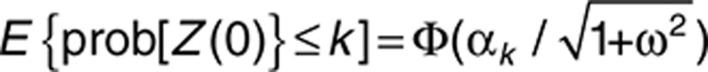
Probit regression can, however, allow a convenient analytical determination of the model-predicted average probabilities. With η representing the only random effect in Eq. 1, and let q_k = β_k − M(t) be the fixed-effect term, the expected probability is given as follows⁶:

Exposure–Response Modeling

Exposure–response (E-R) modeling can facilitate effective dosing decisions.⁷ For categorical end point modeling, M(t) in Eq. 1 needs to be chosen as a function of drug exposure. It may be easy to consider linear functions of some observed systemic exposure measures, such as trough drug concentrations, area under the curve (AUC), or log(AUC) at or prior to certain time points, e.g., week 24 in the motivating example. More mechanism-based approaches have also been used. Although exact distinctions could be difficult, some major characteristics of empirical and mechanism-based approaches are elaborated below.

Empirical approaches

Using observed exposure metrics such as AUC leads to direct correlations between observed end points and exposure measures, which may be the simplest and thus perhaps more often used approach in clinical development. Such correlations describe the data from which they are built, by default. However, as a general principle, data at hand are already known, thus the more important question is under what circumstances the model is likely to predict well. Under linear pharmacokinetics, such correlations could be used to determine dose–response relationships when the dosing frequency is fixed, with the observed exposure measures serving as surrogates for the overall exposure profile. When the pharmacodynamics is fast relative to the pharmarcokinetic half-lives, the empirical correlation may be mechanistically interpretable. However, in the more common situations where there are delays between measured concentrations and effects, these correlations generally will not hold under different dosing frequencies or administrative routes. For example, in the above motivating example, relationships between the concentration and ACR20 at week 24 in principle will differ between the q8-weeks and the q12-weeks regimens. In addition, the direct correlations typically may be built with only fractions of all observed E-R data, such as the measured concentrations and ACR assessments at week 24, again because the relationships likely will differ for different time points such as week 8 or week 16. In phase II, categorical response data are often too sparse to allow precise quantification of such relationships, e.g., the concentration–ACR20 response at a particular time point.

Likewise, the recently emerging Markov transition models, while having been shown to describe the data well, may have limited predictive ability. To realize this, it may help to consider that for continuous end points, why a current observation is typically not modeled based on a previous one. From a mechanistic viewpoint, responses are determined by the pharmacodynamics characteristics and the exposure time course. These may not be fully represented by the immediate past responder/nonresponder status and the current drug concentration level. In the motivating example, the ACR20 response at week 24 should be determined by the exposure time course between weeks 0 and 24 and the pharmacodynamic delay characteristics, which may not be fully represented by the ACR20 responder status at week 20 and the drug concentration at week 24.

Mechanism-based approaches

Mechanism-based models extrapolate better across varieties of scenarios and can be built using all available data. With limited data in practice, care should be taken to include the crucial features that are supportable. As a general principle, the modeling approach used should be determined in conjunction with the intended use of the model. In practice, the least empirical or most interpretable, flexible model that can be supported by the data should typically be used.

Dosing selection generally requires the models to extrapolate across different dosing frequencies and administrative routes. This typically requires modeling the delay between systemic exposure and clinical response, along with the placebo effect. These features ideally should be incorporated in a principled and natural way. A class of E-R models suitable for this purpose is the widely used types I–IV indirect response (IDR) models.⁸ For clinical end points, more complex models are not likely to be effectively estimated in late developmental stages.

Indirect response models

IDR models may be generally described as follows⁸: let the response be R = R(t), with baseline R(0) = R₀, then:

where H₁(t) and H₂(t) take the form of E_maxC(t)/[C₅₀ + C(t)] where C(t) is drug concentration and C₅₀ and E_max are model parameters. For type I and type III IDR models, E_max = −I_max or S_max represents the maximum inhibitory or stimulation effect, respectively, and H₂(t) = 0. For type II and type IV IDR models, E_max = −I_max or S_max, respectively, and H₁(t) = 0. Model equations for various baseline-normalized IDR models have been derived, including reduction-from-baseline (R₀–R) and ratio-of-baseline (R/R₀).^2,9 They allow the applications of alternatively parameterized IDR models to clinical end points.²

Although originally designed for physiological variables, the IDR models may be viewed as collapsed versions of more complex mechanistic models.³ This important fact facilitates the interpretation of IDR models in a broad range of applications and supports their predictive ability.

Latent Variable Representation

The logistic/probit regression model in Eq. 1 may appear empirical, thus making it unclear how best to incorporate any mechanism-based models into the predictor M(t). For example, it may seem equally reasonable to use either M(t) = R(t) or another function such as M(t) = log[R(t)], with R(t) being an IDR model. To select mechanism-consistent model forms, it is important to realize that logistic and probit regressions may be motivated by conceiving an unobservable, hence latent, physiological variable. The latent variable represents the underlying cause such that when it crosses certain thresholds, it causes the observed response to fall in the respective categories.⁴ Then, IDR models may be applied to the latent variable.

To derive the latent variable representation, let L(t) be the latent variable and {β_k} be the thresholds such that

Assume that L(t) is modeled as

where M(t) is the model predictor, ɛ ~ N(0, σ²) follows the standard normal distribution, and σ is the error SD. For notational convenience of this derivation, BSV are assumed to be contained in M(t). Then,

When the model specification for M(t) includes a multiplicative parameter, σ will not be separately identifiable and may be assumed to equal 1, and the above can be written as

which corresponds to probit regression, with Φ⁻¹ as the inverse of the cumulative normal distribution function. Logistic regression in the same form may be similarly derived by assuming the logistic distribution instead of the normal. While standard in statistical theory,⁴ in the context of applying IDR models, this derivation was first given by Hutmacher et al.³ The derivation allows the interpretation of M(t) in Eq. 1 as a physiological variable, and consequently, the mechanistic consistency of applying IDR models to M(t).

Incorporating the placebo effect

Clinical trials typically include placebo arms. The placebo treatment may also take the form of an active standard therapy, and the trial evaluates the add-on effect of the investigational drug. If the placebo period is sufficiently long, the effect may attenuate from its peak. This could be due to multiple reasons, including regression to the mean. However, most often, the attenuation is not observed during the course of the trial, especially for large clinical trials. Placebo effect is typically modeled empirically and, for simplicity, is assumed beneficial and increasing-in-time in this article. The 1-pathway and 2-pathway approaches, elaborated below, have been used to incorporate placebo effect under IDR models. They differ in interpretation and ease of implementation.

1-Pathway. This approach may be the easier one to conceive in order to incorporate placebo effect under the standard IDR model form of Eq. 3. It applies IDR models directly to M(t) and then models the placebo effect on a parameter, typically on k_in, e.g., as k_in(t) = k_in,0[1 - P_max exp(-r_p t)]. A latent variable approach in this form was applied to ACR20, ACR50, and ACR70 by Hu et al.¹⁰ and subsequently used with a more complex physiological model by Ait-Oudhia et al.¹¹ The placebo model parameters cannot be separately estimated from placebo data alone. This may create difficulty for finding good initial parameter estimates as well as stable overall parameter estimation.

2-Pathway. This approach separates the placebo and drug effect terms. A convenient choice is:

where f_p(t) and f_d(t) correspond to placebo and drug effect, respectively, and at baseline f_p(0) = 0. Then, IDR models can be used for f_d(t). The ease of parameter estimation of the 2-pathway approach may depend on the parameterization chosen, as shown below.

Combining Eqs. 1 and 5 gives:

Early applications substituted R(t) in Eq. 3 for f_d(t) and directly estimated the model parameters in this form.³ However, when no drug is given, f_d(t) = f_d(0) = R₀ > 0, therefore, f_d contains the drug effect as well as a component of baseline, and again, the placebo model parameters are not separately identifiable from placebo data, as with the 1-pathway approach. On the other hand, Eq. 6 could be rewritten, or reparameterized, as:

Writing α_k = β_k − R₀, g_p(t) = −f_p(t), and letting R₁(t) = [R₀ − f_d(t)] be the corresponding reduction-from-baseline IDR model, then

where g_p(t) may be empirically modeled with g_p(0) = 0. Furthermore, R₁(t) is shown by Hu et al.² to satisfy

The interpretation of the parameters in the reparameterized form Eqs. 7–8 can be compared with those in Eqs. 6 and 3. Some remain the same and retain their interpretations; the BSV and placebo effect terms are identical, as are the IDR model parameters, including R₀ which represents the baseline latent variable value via Eq. 5. However, the interpretation of the constant terms changes; while β_k in Eq. 6 represent latent variable thresholds, α_k in Eq. 7 have the empirical interpretation as intercepts, representing baseline probabilities (along with BSV). When no drug is given, R₁(t) = 0 in Eq. 7, therefore, the remaining terms [η + α_k + g_p(t)] represent placebo response so that the related parameters can be separately estimated from placebo data. This is advantageous for stable parameter estimation.

Hu et al.^2,12,13 proved that Eqs. 7–8 were equivalent to the latent variable IDR model in their earlier applications. The earlier model^13,14 was motivated somewhat heuristically to apply the IDR model in a way that allows the placebo effect parameters to be separately estimated from placebo data. The proof showed that R₀ was equivalent to the maximum drug effect parameter in the earlier application when the maximum inhibitory or stimulation effect E_max = 1. Eqs. 7–8 also relate more directly to the standard IDR model forms than the earlier model.^13,14 Most importantly, the latent variable interpretation of Eqs. 7–8 substantiates the approach with mechanistic consistency, thereby strengthening its applications.

The mechanistic rationale of the 1-pathway approach could be questionable, as it is often difficult to justify why placebo (or the active control) would affect the same pathway. In contrast, under the 2-pathway approach, the total drug and placebo effect may be interpreted as the sum of those from the drug pathway and other nonspecific pathways.¹⁵ Because of this and the earlier mentioned advantage of stable parameter estimation, the 2-pathway approach will be the focus of the remainder of this article.

Change-From-Baseline End Points

Clinical end points may represent various types of change from baseline in disease conditions, such as the Likert scale measures for patient reported outcomes, DAS28 response criteria (defined according to the magnitude of DAS28 improvement from baseline and by baseline DAS28 categories) in rheumatoid arthritis, and ACR20, ACR50, and ACR70.^16,17 The definitions of these end points suggest that they may be considered as arithmetic change, proportional change, and percent improvement from baseline in nature, respectively. These different natures conceivably could change how the underlying latent variables influence the clinical end points, thus affecting how they should be modeled. Addressing this issue requires latent variable model derivations according to each end point type, which are given in the Supplementary Appendix. The derivations show that the latent variable model in Eqs. 7–8 may suit these various types of change-from-baseline clinical end points, and thus retain their mechanistic consistency.

Placebo Model Interpretation and Choice

At baseline, g_p(0) = R₁(0) = 0 in Eq. 7. For probit regression, this implies q_k = α_k in Eq. 2, and

Thus, the baseline probabilities can be directly computed from the intercepts along with the BSV variance, a fact that also holds for logistic regression although simulation calculations are necessary. This fact allows approximate initial estimates of intercepts α_k to be obtained from observed baseline response (by first selecting a reasonable initial estimate of ω). Similarly, if g_p(∞) = P_max, the term (α_k − P_max) represent average steady-state placebo probabilities, thus an approximate initial estimate of P_max may be conveniently obtained if the placebo response plateau is observed.

It is noted that the placebo model parameters generally should still be jointly estimated with drug effect parameters from all data to gain estimation efficiency. Nevertheless, as mentioned earlier, obtaining these initial estimates is an advantage of the reduction-from-baseline IDR model parameterization (Eqs. 7–8). In contrast, with the original parameterization (Eqs. 6 and 3), because α_k = β_k − R₀, the parameters β_k and R₀ cannot be separated. That is, the original parameterization does not allow any subset of parameters to be estimated with a subset of the data.

A convenient choice of the placebo model in Eq. 7 takes the exponential form:

where P_max is maximum effect and r_p is rate of onset.

Alternative equivalent placebo model

In case that the placebo model in Eq. 7 will plateau, it may be reparameterized as follows: let α_k′ = α_k + g_p(∞), h_p(t) = g_p(t) − g_p(∞), then α_k + g_p(t) = α_k′ + h_p(t), and Eq. 7 becomes

where α_k′ are threshold parameters to be estimated and h_p(t) is constrained with h_p(∞) = 0. This shows that in Eq. 7, the alternative constraint of g_p(∞) = 0 may be taken instead of g_p(0) = 0. A convenient choice in this form is

This reparameterization changes the interpretation of the threshold parameters (along with the BSV variance) from representing average probabilities at baseline to representing average probabilities at steady state. This could lead to more stable parameter estimation, in case the plateau of placebo response is observed sufficiently long at steady state.

Placebo model reduction

For change-from-baseline end points, Hu et al.² proposed a reduced model restricting the baseline probability prob[Z(0) ≤ k] = 0, in the following form:

which has one parameter less than Eq. 9 or Eq. 10. The motivation and interpretation are given in the Supplementary Appendix. The reduced model may be more preferable especially for small to moderate data sizes. The choice may ultimately depend on how much complexity the data can support, i.e., goodness of fit. In the motivating example, observed data (Figure 1 of Hu et al.²) indeed suggest that one parameter may be sufficient to describe the placebo response time course. When in doubt, testing both Eq. 11 and Eq. 10 may be prudent.

Indirect Response Model Usage

In the latent variable framework, the maximum inhibitory or stimulation effect E_max, i.e., −I_max or S_max in the general IDR model representation Eq. 3, is usually not separately estimable from the remaining IDR model parameters and should be set to 1. Some earlier applications tested this explicitly.² A heuristic argument is given below. Consider a steady-state infusion that maintains concentration C(t) at C_ss and the drug effect R₁(t) at R_ss. Setting the left side of Eq. 8 equal to 0 gives:

Solving this for R_ss gives:

For type I and type III IDR models, this leads to

therefore, R₀ and E_max are not separately identifiable.

For type II and type IV IDR models,

so that R₀ and E_max are indistinguishable and so are C₅₀ and E_max.

Extensions to Continuous End Points

When the number of clinical response categories becomes large, the end point may often be treated as continuous. Existing applications typically apply IDR models directly to the end point, often using the 1-pathway approach to model the placebo effect.¹⁸ The difference between 1- and 2-pathway models have been discussed.³ The latent variable model derivation may be extended to this case by treating the latent variable L(t) as the observed response Z(t). Specifically, combining Eqs. 4 and 5 and using a similar baseline reparameterization as in the derivation leading to Eq. 7 gives the following continuous end point analog:

where R₁(t) satisfies Eq. 8, and BSV may be placed on more parameters in addition to baseline b. The placebo effect g_p(t) may still be modeled with the exponential model Eq. 9. Eq. 12 is equivalent to some existing applications; however, the 2-pathway reduction-from-baseline model parameterization may still allow clarity in interpretation and stable estimation.

Hutmacher et al.¹⁵ argued that the actual physiological mechanism may collapse to any of the four IDR models, and therefore, all IDR models should be tried. In the general setting of modeling continuous and ordered categorical clinical end points, Hu et al.² proved a symmetry between type I and type III IDR models when the link function is symmetric. The symmetry is motivated by the observation that drug effects on clinical end points can be modeled either as reducing harmful effects or as increasing beneficial effects. For example, in the motivation example, the drug effect can be modeled in either of the two approaches: (i) increasing the probability of achieving ACR responses and (ii) reducing the probability of failing to achieve ACR responses. The symmetry states that using type I/III IDR models in approach (i) is equivalent to using type III/I models in approach (ii) in that the two approaches will result in identical model predictions along with corresponding IDR model parameters. This result is general because most practically used link functions are symmetric, including the logit, probit (Eq. 7), and the identity or minus-identity (Eq. 12) links. Therefore, there are only three IDR models to be tried when modeling clinical end points.

Other Extensions

Two possible further applications are briefly described below.

Lognormal error latent variable

Conceivably, L(t) as the underlying physiological variable should be positive, which motivates the lognormal error model L(t) = M(t) exp(σɛ). Incorporating the placebo effect multiplicatively as M(t) = f_p(t) f_d(t), a derivation similar to that of Eqs. 7–8 leads to:

where D_e is a model parameter, and R₂(t) satisfies the ratio-of-baseline IDR model form⁹:

A convenient choice for the placebo model g_p(t) is again Eq. 9.

The lognormal error model Eqs. 13–14 could be considered as inferior to the normal error model Eqs. 7–8 due to conceptual reasons. On the other hand, it is interesting to compare Eq. 13 with the earlier model used by Hu et al.^2,12,13 Those were the same as Eq. 13 with the term D_elog[R₂(t)] replaced by a first-order Taylor expansion D_e[1 − R₂(t)]. Therefore, models Eqs. 7–8 and Eqs. 13–14 may be expected to perform similarly when [1 − R₂(t)] is small, i.e., drug effect is substantial. The author's limited experience to date with data used in early applications was consistent with this notion.^2,13,14 Further confirmation is necessary.

Correlation between multiple end points

Clinical trials may have multiple end points, and the magnitude of raw correlation between the end points indicates the similarity level between the disease components that the end points are designed to measure. Jointly modeling the end points allows the identification of common model parameters and BSVs or, in the case of simultaneous modeling of continuous and categorical end points, a latent structure that can predict both the continuous and categorical end points. After this, extra correlations between the end points unaccounted for by BSVs may still remain and can be by the correlations among (latent) variables. In principle, this improves overall estimation efficiency (C. Hu, P. Szapary, A. Mendelsohn, and H. Zhou, personal communication).⁶

The standard approach to model the extra correlation uses the multivariate normal distribution. Although the probit latent variable approach allows it, the distribution is not currently available in the common E-R modeling software NONMEM. This can however be implemented with a conditional approach that factorizing the joint likelihood as the product of the likelihood of one variable with the conditional likelihood of the other (C. Hu, P. Szapary, A. Mendelsohn, and H. Zhou, personal communication). The magnitude of extra correlation can suggest whether the marginal end point models sufficiently accounted for the information in the individual end point data, thus providing a diagnostic on the quality of the marginal models.

Estimation and Diagnostics

This section illustrates some related practical topics. The discussion pertains to general pharmacometric applications of nonlinear mixed-effect models, unless explicitly restricted to latent variable models.

Parameter estimation

Eq. 1 falls under the class of nonlinear mixed-effect models, which require approximations for likelihood-based parameter estimation. E-R analyses often use the software NONMEM with the LAPLACIAN approximation option, although more advanced estimation options such as the stochastic approximation expectation-maximization (SAEM) and importance sampling (IMP) have recently been included.¹⁹ Hutmacher et al.⁶ have investigated the influence of additional estimation methods, including Gaussian quadrature, with latent variable models. The advanced methods have better theoretical characteristics but are more complex and time consuming. Using the LAPLACIAN option may be fine when no obvious lack-of-fits are present. Investigating on advanced methods, even if applied only at the final stage for robustness check, could be helpful. A sample NONMEM code is given in Supplementary Data.

Evaluating estimation uncertainty

Estimation uncertainty is typically assessed with SEs of parameter estimates. Confidence intervals (CIs) are also commonly used. Statistical theory states that with large sample sizes, CIs may be computed from SEs, e.g., the 95% CI may be calculated from ±Φ⁻¹(0.975) * SE = ±1.96 * SE. This requires the so-called asymptotic normality assumption to hold, which is usually difficult to verify. In practice, it is not uncommon to see CIs so computed to be less than zero for parameters with positive ranges. Log transforming these parameters may be an easy way to improve the behavior of the CIs. Nevertheless, SEs for nonlinear mixed-effect models are known to be approximate; therefore, alternative assessments may be desirable.

Bootstrap is currently the most computationally intensive and yet the most popular method used to evaluate model estimation. It is implemented by repeatedly resampling the subjects in the population with replacement and repeating the estimation step and then examining the distribution of the resulted parameter estimates. The percentiles (e.g., 2.5 and 97.5%) of the distribution form natural CIs (e.g., 95%) of the original model parameter estimates. The essence of the methodology is to use resampled subject population to approximate the true population.²⁰ This concept may not have received due recognition of importance, since the appropriateness of resampled population is determined by the stratification variables, but these seem rarely exactly described and justified in typical bootstrap result reporting. In general, the true target population is specified not only by the subjects in the data but also by any covariates used to stratify the resampling, e.g., studies (when data from multiple studies are pooled together) or body weight categories. For the bootstrap results to indicate the true estimation uncertainty, it is thus important to stratify according to study design factors (which typically should be the studies and the study-specified stratification variables) and to ensure sufficient number of subjects in each stratum.^10,21

Likelihood profiling is another method to obtain CIs and understand the skewness of the estimation uncertainty. It assesses one parameter at a time and can be motivated from likelihood ratio tests. The assessed parameter is fixed at different values adjacent to the original parameter estimate, with the likelihood function maximized with respect to the remaining model parameters. The resulted objective function (−2 times the maximum log likelihood) values can then be numerically examined and plotted vs. the fixed values of the parameter assessed, and CIs may be obtained by finding the parameter values that correspond to the desired nominal changes of objective function values. This has been used in latent variable IDR model applications.^2,10 Without concerns about stratifications and yet typically requiring fewer model runs, likelihood profiling may be viewed as an efficient alternative to bootstrap.

Model diagnostics

Few generally useful goodness-of-fits are available for categorical data. The visual predictive check (VPC)²² may be the most useful and can be effectively implemented by plotting the observed frequencies of response vs. prediction intervals (e.g., 90%) of the model. For binary data, the issue of grouping the data by covariates has been discussed.²³ For E-R modeling of clinical trial data, a natural way to group the responses is by study visit and treatment,^{2,10,12,13,14} due to the importance of understanding the treatment response frequencies over planned time course in dosing regimen selection.

Model validation

Model validation may be a confusing term. In the previous decade, models were often claimed as “validated” after showing similarity between the means or medians of the distribution of bootstrapped parameter estimates and the original model parameter estimates, before Hu et al.¹⁰ proved that such similarity can be expected to regularly occur despite arbitrarily large biases. Although the general use of bootstrap, jackknife, and cross-validation approaches do have the potential, implementation in the mixed-effect modeling will require much more sophistication.²⁰ In a strict sense, model validation concerns with predictive ability which, to avoid subjectivity, could be assessed only with newly arrived data. Furthermore, because nonlinear mixed-effect models have multiple components, it is often unclear which ones should or could be validated for the particular application. For example, because the random-effect component (i.e., BSV) is not directly observed, it is usually difficult to validate the related components such as covariate models with sparse sampling due to the lack of sound practical metrics to evaluate the difference between model-predicted and “observed” parameters since empirical Bayes estimates are not mutually independent.

For the purpose of dosing regimen decisions, the most important quantity is likely the time course of clinical response probabilities. Obtaining new data solely for the purpose of model validation may be difficult in early development, e.g., proof-of-concept stages. This should be possible in later development stages, where data from new trial(s) can be used to conduct external VPCs of the model developed.¹⁴ The performance, especially if the validation data contain new dosing regimens, can conveniently provide a natural and objective assessment of the predictive ability of the model.

Suggested Latent Variable Model Development Steps

Latent variable IDR model development may often be relatively straightforward using data from placebo-controlled clinical trials where drug concentrations and clinical responses are measured at multiple time points. Reasonable models could be developed with the following main steps:

• Plot placebo data. Fit exponential model Eq. 9 to obtain initial estimates of placebo effects.

• Fit selected IDR model with Eqs. 7 and 8.

• Plot mean predictions vs. means of the data or examine VPC as diagnostics.

The alternative placebo model Eq. 10 may be used instead of Eq. 9 if the placebo response time course appears to have plateaued. The reduced placebo model Eq. 11 can be used and tested in steps 1 and 2, when the response reflects change from baseline. All three types of IDR models (type I/III, II, and IV) may also be tested.¹⁵ If additional data become available after initial model development, external VPC can be performed for model validation before pooling in the new data and re-estimate the model. Additional assessment of estimation uncertainty, e.g., likelihood profile or bootstrap, may be conducted.

As an illustration, the E-R model development of the motivating example is briefly summarized below. In step 1, plotting the placebo data trend (Figure 1 of Hu et al.²) suggested that 1-degree of freedom of the reduced model Eq. 11 could suffice and was confirmed by VPC of the initial placebo logistic regression model. Next, parameter estimates of a type I latent variable IDR model with Eqs. 7–8 were obtained. The VPC (Figure 2 of Hu et al.²) showed reasonable model description of observed data. The more complex placebo effect model Eq. 9 did not significantly improve the fit. Comparing the initial placebo model and the final model parameter estimates and VPCs showed that the minor differences between parameter estimates did not affect model description of placebo data. Finally, likelihood profile plots (Figure 4 of Hu et al.²) showed reasonable precision of IDR model parameters but high uncertainties in some placebo effect parameters. This supported the importance of parsimony, perhaps especially for the placebo effect model, even in this case of large phase III trials with reasonable sample sizes. Finally, the model was used to simulate possible time courses of ACR response probabilities under multiple alternative dosing regimens (Figure 5 of Hu et al.²) for dosing justification. In contrast, plotting the response probabilities in observed trough concentration quartile ranges suggested difficulties in identifying meaningful relationships for the direct correlation approach.²

Discussion

A general latent variable framework is described for clinical end point modeling that allows the utilization of all observed E-R data and better predictive ability, in comparison with some more empirical approaches. The framework is shown to suit the major types of clinical end points and may motivate additional models. The baseline-normalized model parameterization shows advantages in estimation stability. Extra-correlation between end points may be accommodated in this framework using probit regression. Logit regression may be equally effectively used for single end point modeling.

Mechanism consistency allows effective predictions of different dosing regimen outcomes. The presentation here focused on IDR models, but models based on other mechanisms can be used if desired. Note that for the predictions to be robust, especially in phase II when data are relatively sparse, the models should be parsimonious and have practically interpretable parameters. As attributed to Einstein, “everything should be made as simple as possible, but no simpler.” For dosing regimen decisions, the important factors in E-R modeling typically are: baseline, placebo maximum effect and rate of onset, and drug maximum effect and rate of onset. These correspond exactly to the latent variable IDR model parameters, e.g., ({α_k}, P_max, r_p, R₀, and k_out) in Eqs. 7–9. In this sense, the latent variable IDR models may often be expected to be optimal for dosing regimen decisions in clinical drug development. Model building and assessment could often be relatively straightforward.

Conflict of Interest

The author declared no conflict of interest.

References

- Felson D.T., et al. American College of Rheumatology. Preliminary definition of improvement in rheumatoid arthritis. Arthritis Rheum. 1995;38:727–735. doi: 10.1002/art.1780380602. [DOI] [PubMed] [Google Scholar]
- Hu C., Xu Z., Mendelsohn A.M., Zhou H. Latent variable indirect response modeling of categorical endpoints representing change from baseline. J. Pharmacokinet. Pharmacodyn. 2013;40:81–91. doi: 10.1007/s10928-012-9288-7. [DOI] [PubMed] [Google Scholar]
- Hutmacher M.M., Krishnaswami S., Kowalski K.G. Exposure-response modeling using latent variables for the efficacy of a JAK3 inhibitor administered to rheumatoid arthritis patients. J. Pharmacokinet. Pharmacodyn. 2008;35:139–157. doi: 10.1007/s10928-007-9080-2. [DOI] [PubMed] [Google Scholar]
- McCullagh P., Nelder J.A.Generalized Linear Models2nd end., (Chapman & Hall/CRC; London; 1989 [Google Scholar]
- Capuano A.W., Dawson J.D. The trend odds model for ordinal data. Stat. Med. 2013;32:2250–2261. doi: 10.1002/sim.5689. [DOI] [PMC free article] [PubMed] [Google Scholar]
- Hutmacher M.M., French J.L. Extending the latent variable model for extra correlated longitudinal dichotomous responses. J. Pharmacokinet. Pharmacodyn. 2011;38:833–859. doi: 10.1007/s10928-011-9222-4. [DOI] [PubMed] [Google Scholar]
- Pinheiro J., Duffull S. Exposure response–getting the dose right. Pharm. Stat. 2009;8:173–175. doi: 10.1002/pst.401. [DOI] [PubMed] [Google Scholar]
- Dayneka N.L., Garg V., Jusko W.J. Comparison of four basic models of indirect pharmacodynamic responses. J. Pharmacokinet. Biopharm. 1993;21:457–478. doi: 10.1007/BF01061691. [DOI] [PMC free article] [PubMed] [Google Scholar]
- Woo S., Pawaskar D., Jusko W.J. Methods of utilizing baseline values for indirect response models. J. Pharmacokinet. Pharmacodyn. 2009;36:381–405. doi: 10.1007/s10928-009-9128-6. [DOI] [PMC free article] [PubMed] [Google Scholar]
- Hu C., Xu Z., Rahman M.U., Davis H.M., Zhou H. A latent variable approach for modeling categorical endpoints among patients with rheumatoid arthritis treated with golimumab plus methotrexate. J. Pharmacokinet. Pharmacodyn. 2010;37:309–321. doi: 10.1007/s10928-010-9162-4. [DOI] [PubMed] [Google Scholar]
- Ait-Oudhia S., Lowe P.J., Mager D.E. Bridging clinical outcomes of canakinumab treatment in patients with rheumatoid arthritis with a population model of IL-1β kinetics. CPT. Pharmacometrics Syst. Pharmacol. 2012;1:e5. doi: 10.1038/psp.2012.6. [DOI] [PMC free article] [PubMed] [Google Scholar]
- Hu C., Xu Z., Zhang Y., Rahman M.U., Davis H.M., Zhou H. Population approach for exposure-response modeling of golimumab in patients with rheumatoid arthritis. J. Clin. Pharmacol. 2011;51:639–648. doi: 10.1177/0091270010372520. [DOI] [PubMed] [Google Scholar]
- Hu C., Yeilding N., Davis H.M., Zhou H. Bounded outcome score modeling: application to treating psoriasis with ustekinumab. J. Pharmacokinet. Pharmacodyn. 2011;38:497–517. doi: 10.1007/s10928-011-9205-5. [DOI] [PubMed] [Google Scholar]
- Hu C., Szapary P.O., Yeilding N., Zhou H. Informative dropout modeling of longitudinal ordered categorical data and model validation: application to exposure-response modeling of physician's global assessment score for ustekinumab in patients with psoriasis. J. Pharmacokinet. Pharmacodyn. 2011;38:237–260. doi: 10.1007/s10928-011-9191-7. [DOI] [PubMed] [Google Scholar]
- Hutmacher M.M., Mukherjee D., Kowalski K.G., Jordan D.C. Collapsing mechanistic models: an application to dose selection for proof of concept of a selective irreversible antagonist. J. Pharmacokinet. Pharmacodyn. 2005;32:501–520. doi: 10.1007/s10928-005-0052-0. [DOI] [PubMed] [Google Scholar]
- Zou K.H., Carlsson M.O., Quinn S.A. Beta-mapping and beta-regression for changes of ordinal-rating measurements on Likert scales: a comparison of the change scores among multiple treatment groups. Stat. Med. 2010;29:2486–2500. doi: 10.1002/sim.4012. [DOI] [PubMed] [Google Scholar]
- Arnett F.C., et al. The American Rheumatism Association 1987 revised criteria for the classification of rheumatoid arthritis. Arthritis Rheum. 1988;31:315–324. doi: 10.1002/art.1780310302. [DOI] [PubMed] [Google Scholar]
- Yates J.W., Das S., Mainwaring G., Kemp J. Population pharmacokinetic/pharmacodynamic modelling of the anti-TNF-α polyclonal fragment antibody AZD9773 in patients with severe sepsis. J. Pharmacokinet. Pharmacodyn. 2012;39:591–599. doi: 10.1007/s10928-012-9270-4. [DOI] [PubMed] [Google Scholar]
- Beal S.L., Sheiner L.B., Boeckmann A., Bauer R.J. NONMEM User's Guides (1989–2009) Icon Development Solutions; Ellicott City, MD, USA; 2009. [Google Scholar]
- Efron B., Tibshirani R.J. An Introduction to the Bootstrap. CRC Press; New York; 1994. [Google Scholar]
- Hu C., Moore K.H., Kim Y.H., Sale M.E. Statistical issues in a modeling approach to assessing bioequivalence or PK similarity with presence of sparsely sampled subjects. J. Pharmacokinet. Pharmacodyn. 2004;31:321–339. doi: 10.1023/b:jopa.0000042739.44458.e0. [DOI] [PubMed] [Google Scholar]
- Holford N.H.G.The visual predictive check - superiority to standard diagnostic (rorschach) plots . < http://www.page-meeting.org/default.asp?abstract=738 >.
- Pavan Kumar V.V., Duffull S.B. Evaluation of graphical diagnostics for assessing goodness of fit of logistic regression models. J. Pharmacokinet. Pharmacodyn. 2011;38:205–222. doi: 10.1007/s10928-010-9189-6. [DOI] [PubMed] [Google Scholar]
Associated Data
This section collects any data citations, data availability statements, or supplementary materials included in this article.