Optimal Multiple Surface Segmentation With Shape and Context Priors

Abstract

Segmentation of multiple surfaces in medical images is a challenging problem, further complicated by the frequent presence of weak boundary evidence, large object deformations, and mutual influence between adjacent objects. This paper reports a novel approach to multi-object segmentation that incorporates both shape and context prior knowledge in a 3-D graph-theoretic framework to help overcome the stated challenges. We employ an arc-based graph representation to incorporate a wide spectrum of prior information through pair-wise energy terms. In particular, a shape-prior term is used to penalize local shape changes and a context-prior term is used to penalize local surface-distance changes from a model of the expected shape and surface distances, respectively. The globally optimal solution for multiple surfaces is obtained by computing a maximum flow in a low-order polynomial time. The proposed method was validated on intraretinal layer segmentation of optical coherence tomography images and demonstrated statistically significant improvement of segmentation accuracy compared to our earlier graph-search method that was not utilizing shape and context priors. The mean unsigned surface positioning errors obtained by the conventional graph-search approach (6.30 ± 1.58 μm) was improved to 5.14 ± 0.99 μm when employing our new method with shape and context priors.

I. Introduction

Over the recent years, automated segmentation of medical images became an important tool contributing to medical diagnosis and treatment planning. Despite all the invested effort, accurate segmentation of organs and other structures of interest remains a challenging problem. The main difficulty lies in the following aspects. First, target objects in medical image data often lack strong boundaries. Second, target objects are often surrounded by adjacent tissues with similar intensity profiles. Furthermore, there are often many objects lying in a small region with contextual mutual influence between each other [1], [2].

To resolve these problems, incorporating prior knowledge in the solution process plays an important role. We report a novel algorithm for simultaneous detection of multiple surfaces using both shape and context prior information. Our method is based on our previously reported graph search framework—a globally optimal surface detection method proposed in [3]–[5], which has been successfully applied to a variety of medical imaging applications (e.g., [6]–[9]). The basic idea is to formulate the image segmentation problem as an energy optimization problem, which can be solved by a graph-based method. The original graph search formulation [3], [4] only used weighted nodes in the graph to represent the desired segmentation properties, which limited the ability to incorporate a broader variety of a priori knowledge. In this work, we propose a novel extension to this graph search method. Two additional pair-wise terms are added to the energy function, which encode the shape and context prior information using a set of convex functions. For optimization, new pair-wise terms are enforced by adding specific weighted arcs in the graph. A globally optimal solution is computed by solving a single maximum flow problem in the graph with the solution defining the optimally segmented surfaces.

The remainder of the paper is organized as follows. Section II reviews the related work on image segmentation. Section III presents how to incorporate both shape and context information in the graph search framework using an arc-weighted graph representation. In Section IV, our approach is applied to intraretinal layer segmentation in optical coherence tomography (OCT) images and Section VII discusses the novelty and generality of the proposed framework as well as its limitations. Finally, Section VIII summarizes the presented work. Preliminary results related to this research have been presented in [10] and this paper is a major extension of the previously presented conference paper.

II. Related Work

Many image segmentation problems can be formulated as energy optimization problems. The majority of the methods can be divided in two large groups—the optimization in a continuous space and the optimization on a set of discrete variables. In both groups, the key problem lies in two aspects—how can the information (e.g., shape, context) be encoded into the energy function and how can the corresponding energy function be optimized.

A. Optimization in Continuous Space

Methods based on energy minimization in the continuous space date several decades back. In the framework of active contour models [11], [12], the boundary of the target object was explicitly represented through certain parametrization. These types of segmentations had difficulties to handle multiple object segmentations or topological changes during the optimization process. To solve the problem, level-set based methods were proposed [13], [14], in which the boundary of the target object is given by the zero level set of an embedding function. In the level set segmentation, the shape priors can be incorporated into the embedding functions as described in [15]–[17]. The main drawback of the level-set formulation as well as of parametric deformable models lies in the fact that the corresponding cost functions are usually nonconvex. The optimization process based on gradient descent method may consequently be trapped easily in a local minimal solution. Furthermore, it is rarely known how far the obtained solutions are from the globally optimal ones.

Recently, continuous image segmentation has been formulated as a convex function minimization with guaranteed global optimality [18]–[21]. While a number of attempts have been made, incorporating prior information into the energy function while maintaining convexity remains challenging. Cremers et al. [22] proposed a novel implicit representation of the shape that can be encoded in functionals, which are convex with respect to the shape deformations. The method can only be used for single object segmentation. The Pock et al. method [21] allowed segmentation of multiple objects using a convex relaxation approach. However, no shape prior information was incorporated. In [23], a convex energy function was employed, which incorporated the shape prior information into a multi-region probabilistic segmentation based on an isometric log-ratio transformation. No context prior information between multi-regions has been included in the energy function.

B. Optimization in Discrete Space

In recent years, segmentation through energy minimization in the discrete space has attracted considerable attention in computer vision [24], [25], [4]. Most approaches formulate the problem as a graph-based minimization problem. Nodes in the graph correspond to pixels or control points in the original image. Image intensity information as well as the prior knowledge is encoded by adding arcs with proper weights in the graph. Felzenszwalb [26] used triangulated polygons to represent and detect deformable shapes in images. Schoenemann et al. [27] employed a ratio functional to incorporate the elastic shape priors. Both methods, however, only work for single surface detection in 2-D cases.

One of the most influential advances related to our research is Boykov’s graph cut method [25] for interactive segmentation of N-D images that used the minimum s − t cut strategy. Several algorithms were developed to incorporate shape prior information based on the graph cut method. Freedman et al. [28] devised an interactive shape prior segmentation method based on graph cut algorithms. The graph arc-weights were employed, which contained information about a level-set function of a shape template. Malcolm et al. [29] incorporated the prior shape information from kernel PCA into an iterative graph cut framework. Vu et al. [2] presented a multiple object segmentation framework—the shape energy based on a shape distance function was incorporated via the weights of the arcs connected with the terminals. The major difference between the method reported here and the graph-cut based methods is that our graph construction allows for specific shape constraints, which lead to an easy incorporation of shape prior information. Compared with graph-cut based methods, the proposed framework provides a more local and flexible control. In addition, incorporating context information for simultaneous detection of multiple “mutually” interacting surfaces into the graph-cut framework is nontrivial. Delong and Boykov’s work [30] reported one possible way towards that goal.

Ishikawa’s method [31] for multi-labeled MRF optimization with convex priors is also closely related to our work. While interpreting a configuration of the multi-labeled MRF model as a surface in the corresponding (geometric) graph, Ishikawa’s method can be used to detect only a single optimal surface. In our work, we strive to simultaneously compute multiple mutually interacting optimal configurations (surfaces) with additional context constraints—an approach that enjoys a number of important applications in medical image segmentation. Note that if we interpret the multi-surface segmentation problem in N-D as a single (N + 1)-D surface segmentation problem, the proposed method solves a multi-labeled MRF optimization problem in (N + 1)-D, which can be solved using a similar graph structure as described in [31]. In fact, the additional constraints enforced in our problem can be modeled as a special convex prior. On the other hand, if the constraint of maximum label difference between any two interacting random variables can be relaxed, then our method can handle general convex priors. From the computational point of view, the essential ideas of Ishikawa’s method and our algorithm are the same, that is, to transform the problem as the so-called minimum s-excess problem [32], although the connection was not directly pointed out [31]. Making use of the specific structure of the underlying graph, the minimum s-excess problem can be solved in polynomial time with Ishikawa’s graph construction. We employ Hochbaum’s general algorithm [32] for solving the s-excess problem, allowing negative node costs and a flexible structure of the graph.

Yin et al. [5] have developed a LOGISMOS framework based on the graph-searching approach for knee-joint segmentation of bones and cartilages. Their work was nevertheless limited to using the node-weighted graph representation without shape prior and context prior penalties in the energy function, which fails to make full use of prior information.

III. Graph Search With Shape and Context Priors

A. Review of Original Graph Search Framework

We first briefly recall the original graph search framework as introduced in [4]. The target is to detect multiple surfaces simultaneously, which represent boundaries of 3-D objects in a volumetric image. An on-surface cost is assigned to each voxel in the image for the detection of the surface, which is inversely related to the likelihood that the desired surface contains the voxel. Surface feasibility constraints are also enforced. Specifically, the hard surface smoothness constraint requires that the change of the surface height when moving from one neighboring surface point to the next should be in the certain range. Similarly, the surface distance constraint reflects the allowed minimum and maximum distances between surface pairs. Note that the height of a surface point can be interpreted as a label of a random variable. Then the hard surface smoothness constraint and the hard surface distance constraint correspond to the constraint of maximum label difference between two interacting random variables. The goal of the graph search method is to find the optimal surface set such that 1) each surface satisfies the surface feasibility constraints; 2) the total cost of voxels on surfaces are minimized. The problem is then transformed into a minimum-cost closed set problem by constructing a geometric graph such that the minimum-cost closed set of the graph actually corresponds to the set of surfaces with the minimum cost. (A closed set is a subset of nodes such that no arcs leave the subset and the cost of a closed set is the summation of the costs of all the nodes in the subset.) The surface feasibility constraints are encoded by adding (directed) arcs between nodes in the graph. Finally, the minimum-cost closed set can be found by computing a minimum s-t cut in a closely related graph.

The major limitation of the original formulation lies in the fact that only node weights in the graph representation are used to represent desired segmentation properties, e.g., on-surface costs. The connectedness from one voxel to the voxels on its neighboring columns is basically of equal importance, which prevents taking full advantage of prior information. In some medical applications, the target surfaces have some preferred shape and the distance between neighboring surfaces are relatively consistent between different datasets. The original formulation does not allow the easy incorporation of the prior shape and context knowledge. One possible way to solve the problem is to use varying feasibility constraints learned from the training set, as reported in [8]. However, this method cannot penalize the deviation inside the allowed constraints.

B. Incorporation of Shape and Context Priors

To present our method in a comprehensible manner, let us consider a task of detecting multiple terrain-like surfaces incorporating shape and context prior knowledge. Note that this simple principle used for this illustration is directly applicable to arbitrarily-irregularly meshed surfaces (see Section VII-C). Consider a volumetric image (X, Y, Z) of size X × Y × Z. For each (x, y) pair, the voxel subset { (x, y, z)|0 ≤ z < Z} forms a column parallel to the z-axis, denoted by p(x, y). Each column has a set of neighboring columns for a certain neighboring setting , e.g., the four-neighbor relationship. The target is to find λ terrain-like surfaces, each of which intersects each column p(x, y) at exactly one voxel, as shown in Fig. 1(a). Thus, the terrain-like surface S_i can be defined as a function S_i(x, y), mapping (x, y) pairs to their z-values. An on-surface cost c_i(x, y, z) is assigned to each voxel (x, y, z) for surface S_i, which is inversely related to the likelihood that the desired surface S_i contains the voxel.

Fig. 1.

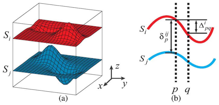
(a) Terrain-like surfaces S_i and S_j intersect each (x, y)-column exactly one time. (b) The shape representation ${\mathrm{\Delta }}_{pq}^i$ between neighboring columns p and q on surface S_i; and the context representation ${\delta }_p^{ij}$ between surfaces S_i and S_j on column p.

1) Shape Prior Constraints

In this paper, the shape changes of surface S_i are defined as the surface height changes between pairs of neighboring columns. Specifically, for any pair of neighboring columns p and q, the shape change of surface S_i between (p, q) relies on ${\mathrm{\Delta }}_{pq}^i=S_i(p)-S_i(q)$ [see Fig. 1(b)]. Suppose ${\overline{\mathrm{\Delta }}}_{pq}^i$ represents the mean shape change learned from certain prior-known shape change model, e.g., Gaussian model. The shape deformation between the current shape change ${\mathrm{\Delta }}_{pq}^i$ and the prior mean shape change ${\overline{\mathrm{\Delta }}}_{pq}^i$ can be expressed as ${\mathrm{\Delta }}_{pq}^i-{\overline{\mathrm{\Delta }}}_{pq}^i$. Two kinds of shape constraints are enforced: the hard shape constraint and the shape prior penalty. The hard shape constraint defines the possible range of the shape deformation with the form: $\mid {\mathrm{\Delta }}_{pq}^i-{\overline{\mathrm{\Delta }}}_{pq}^i\mid \le L_{pq}^i$, where $L_{pq}^i$ is the shape constraint parameter between columns p and q for surface S_i, which is learned from the prior shape change model. The shape-prior penalty is enforced using a convex function $f_s({\mathrm{\Delta }}_{pq}^i-{\overline{\mathrm{\Delta }}}_{pq}^i)$, which penalizes the shape deformation inside the range of the hard shape constraint.

2) Context Prior Constraints

For a set of target surfaces, the context prior penalty is enforced to penalize the surface distance change between two adjacent surfaces. Suppose S_i and S_j are two adjacent surfaces denoted as (S_i, S_j) ∈ , where is a given surface adjacency setting, e.g., two-neighbor relationship in z direction. The context information between (S_i, S_j) on column p is defined as ${\delta }_p^{ij}=S_i(p)-S_j(p)$ [Fig. 1(b)], which is the distance between two surfaces on column p. Let ${\overline{\delta }}_p^{ij}$ denote the mean surface distance obtained from prior context model. The change between current surface distance and the learned mean distance can be represented by ${\delta }_p^{ij}-{\overline{\delta }}_p^{ij}$. Similar to the shape prior constraints, two kinds of context prior constraints are employed. The possible distance between two surfaces (S_i, S_j) are defined by hard context constraints as $\mid {\delta }_p^{ij}-{\overline{\delta }}_p^{ij}\mid \le H_p^{ij}$, where $H_p^{ij}$ is the context constraint parameter for column p between surfaces (S_i, S_j), which is learned from the prior context model. The context-prior penalty is given by a convex function $f_c({\delta }_p^{ij}-{\overline{\delta }}_p^{ij})$ to penalize the surface distance change between current distance and the prior model.

Now the overall energy of the set of λ surfaces S_i’s takes the form

$$E(\mathcal{S})=\sum _{i=1}^{\lambda }\sum _{\mathcal{I}(x,y,z)\in S_i}{c}_i(x,y,z)+\sum _{i=1}^{\lambda }\sum _{(p,q)\in {\mathcal{N}}_c}{f}_s({\mathrm{\Delta }}_{pq}^i-{\overline{\mathrm{\Delta }}}_{pq}^i)+\sum _p\sum _{(i,j)\in {\mathcal{N}}_s}{f}_c({\delta }_p^{ij}-{\overline{\delta }}_p^{ij}).$$ (1)

The first term is the boundary energy term, which is equal to the total on-surface cost of all voxels on surfaces, as used in the original graph search framework. The boundary energy term drives the surface set towards the best fit to the current image data. The second and the third term are the shape-prior penalty term and the context-prior penalty term proposed in this work, which measure how well the surface set fulfills the prior shape change model and the context model, respectively. Using this formulation, we strive to find the optimal terrain-like surfaces such that 1) each surface satisfies the hard shape constraint; 2) each pair of surfaces satisfies the hard context constraints; and 3) the energy in (1) is minimized.

Note that the hard shape constraint and the convex shape-prior penalty can be enforced using Ishikawa’s method [31] with a modified convex function

$$f_s^{\prime }({\mathrm{\Delta }}_{pq}^i-{\overline{\mathrm{\Delta }}}_{pq}^i)=\{\begin{array}{ll}{f}_s({\mathrm{\Delta }}_{pq}^i-{\overline{\mathrm{\Delta }}}_{pq}^i),\hfill & \text{if}\mid {\mathrm{\Delta }}_{pq}^i-{\overline{\mathrm{\Delta }}}_{pq}^i\mid \le L_{pq}^i;\hfill \\ +\infty ,\hfill & \text{otherwise}.\hfill \end{array}$$

The hard context constraint and the context-prior penalty can be enforced in the same way using Ishikawa’s graph construction. In the following Section III-C, we present a slightly different construction of the graph to enforce those constraints, which enables us to apply Hochbaum’s algorithm to solve the general minimum s-excess problem [32].

C. Arc-Weighted Graph Construction

The basic idea for solving the energy minimization problem is to reduce it into a maximum flow problem. A directed graph G containing λ node-disjoint subgraphs {G_i = (N_i, A_i) : i = 1, 2, …, λ} is defined, in which every node n_i(x, y, z) ∈ N_i represents exactly one voxel in (x, y, z).

To enforce the hard geometric constraints, the following arcs with +∞ weight are constructed.

Intra-Column Arcs

To ensure the monotonicity of the target surfaces (i.e., the target surface intersects with each column exactly one time), the intra-column arcs are added as described in [4]. Along every column p(x, y), each node n_i(x, y, z)(z > 0) has a directed arc with +∞ weight to the node immediately below it (i.e., n_i(x, y, z − 1)).

Inter-Column Arcs

The hard shape constraint is incorporated by adding inter-column arcs between neighboring columns in the graph. Specifically, let p(x₁, y₁) and q(x₂, y₂) be two neighboring columns. To enforce the hard shape constraint $\mid {\mathrm{\Delta }}_{pq}^i-{\overline{\mathrm{\Delta }}}_{pq}^i\mid \le L_{pq}^i$, a directed arc with +∞ weight is put from each node n_i(x₁, y₁, z) of p(x₁, y₁) to the node $n_i(x_2,y_2,max(z-{\overline{\mathrm{\Delta }}}_{pq}^i-L_{pq}^i,0))$ of q(x₂, y₂). Note that if $z-{\overline{\mathrm{\Delta }}}_{pq}^i-L_{pq}^i>Z-1$, then voxel I(x₁, y₁, z) cannot be on any feasible surface S_i. To avoid such an invalid surface S_i, we introduce an additional node n_i(x₂, y₂, Z) with an on-surface cost of +∞ and add a directed arc of a +∞ weight from n_i(x₁, y₂, z) to n_i(x₂, y₂, Z). Meanwhile, we have a directed arc with +∞ weight from the node n_i(x₂, y₂, z) to $n_i(x_1,y_1,max(z+{\overline{\mathrm{\Delta }}}_{pq}^i-L_{pq}^i,0))$. If $z+{\overline{\mathrm{\Delta }}}_{pq}^i-L_{pq}^i>Z-1$, we can handle it in the same way as above.

Inter-Surface Arcs

The hard context constraint can be enforced by adding inter-surface arcs between different sub-graphs. Suppose S_i and S_j are two neighboring surfaces. The hard context constraint $\mid {\delta }_p^{ij}-{\overline{\delta }}_p^{ij}\mid \le H_p^{ij}$ on column p(x, y) is incorporated by adding a directed arc with +∞ weight from each node n_i(x, y, z) to the node $n_j(x,y,max(z-{\overline{\delta }}_p^{ij}-H_p^{ij},0))$. Note that if $z-{\overline{\delta }}_p^{ij}-H_p^{ij}>Z-1$, then there is no feasible set of surfaces in which S_i passes voxel I(x, y, z). To avoid such an invalid solution, we introduce an additional node n_j(x, y, Z) with an on-surface cost of +∞ and put a directed arc of a +∞ weight from n_i(x, y, z) to n_j(x, y, Z). On the other hand, each node n_i(x, y, z) also has a directed arc with +∞ weight to the node $n_i(x,y,max(z+{\overline{\delta }}_p^{ij}-H_p^{ij},0))$. If $z+{\overline{\delta }}_p^{ij}-H_p^{ij}>Z-1$, we can handle it in the same way as above.

The remaining challenge is how to incorporate the shape-prior penalty term and the context-prior penalty term into the graph search framework. To solve the problem, additional weighted arcs are introduced in the graph. We start from the incorporation of the shape prior penalties.

Weighted Inter-Column Arcs

Let p(x₁, y₁) and q(x₂, y₂) be two neighboring columns. To “distribute” the convex shape prior penalty $f_s({\mathrm{\Delta }}_{pq}^i-{\overline{\mathrm{\Delta }}}_{pq}^i)$ to arcs between neighboring columns (p, q) in G_i, we make use of the (discrete equivalent of) second derivative of f_s(·) with the form [f_s(h)]″ = [f_s(h + 1) − f_s(h)] − [f_s(h) − f_s(h − 1)]. Since f_s(h) is a convex function, [f_s(h)]″ ≥ 0. Let [f_s(h)]′ = f_s(h + 1) − f_s(h) denote the first derivative of f_s(·). For each $h={\mathrm{\Delta }}_{pq}^i-{\overline{\mathrm{\Delta }}}_{pq}^i$, where $-L_{pq}^i<h<L_{pq}^i$, if [f_s(h)]′ ≥ 0, an arc is added from n_i(x₁, y₁, z) to $n_i(x_2,y_2,z-{\overline{\mathrm{\Delta }}}_{pq}^i-h)$ carrying an arc-weight of [f_s(h)]″. If [f_s(h)]′ ≤ 0, an arc from n_i(x₂, y₂, z) to $n_i(x_1,y_1,z+{\overline{\mathrm{\Delta }}}_{pq}^i+h)$ has the weight of [f_s(h)]″. Fig. 2 shows one typical graph construction. Note that if h = h₀, where [f_s(h₀)]′ = 0, we let ${[f_s(h_0^{+})]}^{″}=f_s(h_0+1)-f_s(h_0)$ for arcs from n_i(x₁, y₁, z) to $n_i(x_2,y_2,z-{\overline{\mathrm{\Delta }}}_{pq}^i-h_0)$ and ${[f_s(h_0^{-})]}^{″}=f_s(h_0-1)-f_s(h_0)$ for arcs from n_i(x₂, y₂, z) to $n_i(x_1,y_1,z+{\overline{\mathrm{\Delta }}}_{pq}^i+h_0)$. Using this construction, it is proved in [3] that the total weight of the arcs that are cut by S_i between two neighboring columns p and q equals to the shape prior penalty represented by convex function $f_s({\mathrm{\Delta }}_{pq}^i-{\overline{\mathrm{\Delta }}}_{pq}^i)$.

Fig. 2.

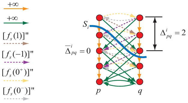
Arc-weighted graph construction for the incorporation of the shape prior penalty on surface S_i between neighboring columns p and q. The intra-column arcs are shown in orange with +∞ weight. The hard shape constraint $\mid {\mathrm{\Delta }}_{pq}^i-{\overline{\mathrm{\Delta }}}_{pq}^i\mid \le L_{pq}^i$ is enforced by green arcs. Here we suppose ${\overline{\mathrm{\Delta }}}_{pq}^i=0$ and $L_{pq}^i=2$. The shape prior penalty is incorporated by arcs with dashed lines (brown, purple, yellow, and gray). Here we assume ${\overline{\mathrm{\Delta }}}_{pq}^i=0$, [f_s(0)]′ = 0 and f_s(0) = 0. Target surface S_i cuts arcs with weight [f_s(1)]″ (brown) and [f_s(0⁺)]″ = f_s(1) − f_s(0) (yellow). The total weight is equal to f_s(2).

Weighted Inter-Surface Arcs

The context-prior penalty is enforced in a similar way by adding weighted inter-surface arcs between corresponding sub-graphs. Suppose S_i and S_j are two adjacent surfaces. The context-prior penalty is distributed between subgraph G_i and G_j on the same column p(x, y). For each $d={\delta }_p^{ij}-{\overline{\delta }}_p^{ij}$, where $-H_p^{ij}<d<H_p^{ij}$, if [f_c(d)]′ ≥ 0, an arc is added from n_i(x, y, z) to $n_j(x,y,z-{\delta }_p^{ij}-d)$ with weight [f_c(d)]″. If [f_c(d)]′ ≤ 0, an arc is assigned from n_j(x, y, z) to $n_i(x,y,z+{\overline{\delta }}_p^{ij}+d)$ with weight [f_c(d)]″. The graph construction is shown in Fig. 3. Using this construction, the total weight of the arcs cut by the surface set between two subgraphs G_i and G_j on column p equals to the context prior penalty $f_c({\delta }_p^{ij}-{\overline{\delta }}_p^{ij})$.

Fig. 3.

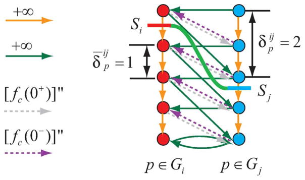
Arc-weighted graph construction for the incorporation of the context prior constraints between surface S_i and surface S_j on column p. Two subgraphs G_i (red) and G_j (blue) are constructed. The hard context constraint $\mid {\delta }_p^{ij}-{\overline{\delta }}_p^{ij}\mid \le H_p^{ij}$ is incorporated by green arcs. Here ${\overline{\delta }}_p^{ij}=1,H_p^{ij}=1$. The context-prior penalty is enforced by gray and purple arcs. We assume that [f_c(0)]′ = 0 and [f_c(0)] = 0. Target surface set S = {S_i, S_j} cuts arcs with weight [f_c(0⁺)]″ (gray). The total weight is equal to f_c(1).

To encode the on-surface cost, the weight of each node in the graph is designed using a similar way as described in [4]. Suppose a voxel I(x′, y′, z′) is on a surface S_i. Then all nodes n_i(x′, y′, z′) with z ≤ z′ on column p(x′, y′) are viewed as being inside the surface S_i. The node weight is assigned such that the total weight of all nodes n_i inside the surface S_i equals to the boundary energy term c_i(x, y, z), where i = 1, …, λ

$$w_i(x,y,z)=\{\begin{array}{ll}{c}_i(x,y,z),\hfill & \text{if}z=0\hfill \\ c_i(x,y,z)-c_i(x,y,z-1),\hfill & \text{if}0<z\le Z-1\hfill \end{array}.$$ (2)

With the constructed graph G, we can find an optimal cut = (A^*, Ā^*) (A^* ∪ Ā^* = N) in G, minimizing the total weight of nodes in A^* plus the total weight of those arcs with their tails in A^* and their heads in Ā^*, which is the so-called minimum s-excess problem [32]. As described in [3] and [32], this optimal cut can be found by solving a maximum flow problem. The optimal cut in the graph uniquely defines optimal λ surfaces in .

IV. Application to Intraretinal Layer Segmentation of OCT Images

The utility of the reported approach will be demonstrated on the automated segmentation of 3-D intraretinal layers in OCT images, an important task in ophthalmic image analysis [8]. The seven intraretinal layers that are identified in our studies are shown in Fig. 4(a) and (b).

Fig. 4.

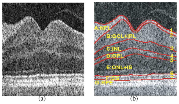
Intraretinal layers in 3-D OCT images. (a) A 2-D slice from the center of a volumetric OCT image—the dip corresponds to the fovea. (b) Seven surfaces (labeled 1–7) and corresponding retinal layers (NFL: nerve fiber layer; GCL+IPL: ganglion cell layer and inner plexiform layer; INL: inner nuclear layer; OPL: outer plexiform layer; ONL+IS: outer nuclear layer and photoreceptor inner segments; OS: photoreceptor outer segments and RPE: retinal pigment epithelium).

A. Workflow

In our application, we employ similar workflow as described in [8]. As the first step, the original images were flattened so that the surfaces near the retinal pigment epithelium layer (RPE) became approximately planar. Then, a two-step intraretinal layer segmentation was performed on 3-D flattened images.

1) Image Flattening

Flattening 3-D OCT images allow us to perform the intraretinal layer segmentation in a truncated region-of-interest of original 3-D OCT image, which reduces time and memory consumption of our graph-based segmentation. Furthermore, it provides a more consistent shape for segmentation and also make visualization easier for clinical use. We used exactly the same approach as described in [8] for image flattening. First, the image was downsampled by a factor of 4. Then surfaces 1, 6, and 7 were simultaneously segmented using the original graph search approach on the down-sampled image, which lead to an approximate segmentation of three surfaces. A thin-plate spline was fitted to an upsampled version of surface 7. After that, all columns of the full-resolution images were translated so that the fitted surface became a flat plane. Then we truncated the flattened OCT image according to the segmented surfaces 1 and 7.

2) Two-Step Intra-Retinal Layer Segmentation

Our segmentation approach was conducted on the flattened and truncated 3-D images. A two-step approach was employed. The surfaces 1, 6, and 7 were segmented in the full resolution image using previously reported graph search approach without incorporating the shape or context prior information. Our new approach in which both the shape and context penalties are incorporated, was used in the second step to simultaneously segment the remaining surfaces 2, 3, 4, and 5. The motivation of the two-step segmentation is as follows. First, simultaneous segmentation of all seven surfaces in 3-D images induces large memory consumption and significant amount of running time. In addition, our new approach needs to introduce new arcs into the graph to encode both shape and context penalties. Simultaneously segmenting all seven surfaces in one step requires to add additional arcs into the graph for all surfaces, which further increases the memory and time complexity (see discussion in Section VII-B). Thus, surfaces 1, 6, and 7 with relatively strong boundaries are segmented using our previous method to avoid unnecessary expense of memory and time complexity. Our new approach with both shape and context penalties was applied on surfaces 2, 3, 4, and 5, which lack clear boundaries and of which substantial inter-surface interactions exist. Fig. 5 shows the main workflow of the employed approach.

Fig. 5.

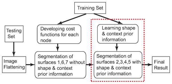
Workflow for OCT intraretinal layer segmentation. The reported approach is utilized in the second step (indicated by the red box) to segment surfaces 2, 3, 4, 5 employing the shape and context priors.

B. Cost Function Design

1) Boundary Cost

For the boundary energy term, we use the gradient-based on-surface costs c_i(x, y, z) for voxels (x, y, z) with respect to surfaces S_i, as reported in [33], [8]. The Sobel kernel was used to favor dark-to-light transitions for surface 4 and light-to-dark transitions for surfaces 2, 3, 5.

2) Shape Prior Model

To incorporate the proper shape prior information, the shape change model is derived from the labeled training dataset (see Section V-A), from which both hard shape constraint and shape-prior penalty function are computed. The distribution of the shape changes ${\mathrm{\Delta }}_{pq}^i$ on the surface i between neighboring columns p and q roughly fits a Gaussian model with the mean ${\overline{\mathrm{\Delta }}}_{pq}^i$ and the standard deviation ${\sigma }_{pq}^i$. To allow 99% of the shape change from column p to column q, the hard shape constraint was set as $\mid {\mathrm{\Delta }}_{pq}^i-{\overline{\mathrm{\Delta }}}_{pq}^i\mid \le 2.6·{\sigma }_{pq}^i$. The shape-prior penalty function $f_s({\mathrm{\Delta }}_{pq}^i-{\overline{\mathrm{\Delta }}}_{pq}^i)$ was designed to penalize the shape change deviation between the current shape change ${\mathrm{\Delta }}_{pq}^i$ and the original shape change model as follows:

$$\begin{array}{l}{f}_s({\mathrm{\Delta }}_{pq}^i-{\overline{\mathrm{\Delta }}}_{pq}^i)=-ln{e}^{-\frac{{\left({\mathrm{\Delta }}_{pq}^i-{\overline{\mathrm{\Delta }}}_{pq}^i\right)}^2}{2{\left({\sigma }_{pq}^i\right)}^2}}\\ =\frac{{\left({\mathrm{\Delta }}_{pq}^i-{\overline{\mathrm{\Delta }}}_{pq}^i\right)}^2}{2{\left({\sigma }_{pq}^i\right)}^2}.\end{array}$$ (3)

3) Context Prior Model

Similar as shape prior model, context prior model is also learned from the segmented training dataset. Specifically, the distribution of distance ${\delta }_p^{ij}$ between surfaces i and j on the column p is approximated using a Gaussian model. Both the mean distance ${\overline{\delta }}_p^{ij}$ and the corresponding standard deviation ${\sigma }_p^{ij}$ are computed from the training sets. The hard context constraint takes the form of $\mid {\delta }_p^{ij}-{\overline{\delta }}_p^{ij}\mid \le 2.6·{\sigma }_p^{ij}$. The context-prior penalty function was set as

$$\begin{array}{l}{f}_c\left({\delta }_p^{ij}-{\overline{\delta }}_p^{ij}\right)=-ln{e}^{-\frac{{\left({\delta }_p^{ij}-{\overline{\delta }}_p^{ij}\right)}^2}{2{\left({\sigma }_p^{ij}\right)}^2}}\\ =\frac{{\left({\delta }_p^{ij}-{\overline{\delta }}_p^{ij}\right)}^2}{2{\left({\sigma }_p^{ij}\right)}^2}.\end{array}$$ (4)

V. Experimental Methods

A. Data

In our study, the same data were used as reported in [8]. Macula-centered 3-D OCT volumes (200 × 200 × 1024 voxels or 6 × 6 × 2 mm³) were acquired from the right eyes of 27 normal human subjects. The 3-D OCT volumes of the right eye of the first 13 subjects were obtained using one OCT device and formed the training dataset. We use exactly the same tracing of training sets as described in [8]. Three steps are involved to produce the segmentation of training sets. Each dataset was firstly divided into 10 regions and one slice was randomly selected from each region. The selected 10 slices were manually traced by one observer. Then a preliminary version of the semi-automatic graph-search segmentation is employed to segment OCT layers based on 10 manually segmented slices. The results were manually edited by the observer to obtain the final tracing for the training sets.

The right eyes of the remaining subjects (14–27) were scanned twice using two different but otherwise identical OCT devices. The obtained 28 volumetric datasets were used for performance assessment. For each 3-D volumetric image in the test set, 10 random slices were traced independently by two ophthalmologists. The averages of these tracings were used as the gold standard for validation.

B. Parameter Setting

As described in Section III, our energy function contained three terms: the boundary term, the shape-prior term and the context-prior term. The combination of these three terms can be described by two parameters α and β as follows:

$$E(\mathcal{S})=E_{\text{boundary}}(\mathcal{S})+\alpha E_{\text{shape}}(\mathcal{S})+\beta E_{\text{context}}(\mathcal{S}).$$ (5)

In our experiments, these two parameters were set as α = 0.9 and β = 0.1, which were determined experimentally based on performance on the training dataset.

C. Shape and Context Prior Model

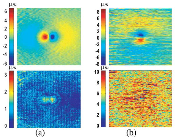
The shape prior model as well as the context prior model were learned from the training set of 13 OCT volumes. Fig. 6 shows the mean and the standard deviation of the shape priors for surface 2 in two directions (e.g., ${\mathrm{\Delta }}_{pq}^i=S_i(x+1,y)-S_i(x,y)$ for the x-direction and ${\mathrm{\Delta }}_{pq}^i=S_i(x,y+1)-S_i(x,y)$ for the y-direction). Fig. 7 illustrates the surface context priors between surface pairs (2,3), (3,4), and (4,5).

Fig. 6.

Visualization of the shape priors for surface 2 learned from the training set. The mean and the standard deviation are shown in the first and second rows, respectively. (a) x-direction. (b) y-direction.

Fig. 7.

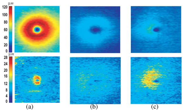
Learned surface context priorsin the form of the mean (the first row) and the standard deviation (the second row) between (a) surfaces (2,3); (b) surfaces (3,4); and (c) surfaces (4,5).

D. Validation

The proposed algorithm was applied to the testing set of 28 volumetric images for validation. The unsigned surface positioning errors were calculated as the distances between the computed surfaces and the surfaces of the gold standard in each column of the image. The results were reported as mean ± standard deviation. The unsigned surface distances between two expert-defined boundaries representing the same retinal surface were considered as the inter-observer variability of the two ophthalmologists. The performance of the proposed method was compared with the inter-observer variability and also with the results report in [8], which used the conventional graph search method with hard constraints only. Statistical significance of the observed differences was determined using Student t-tests for which p values of 0.05 were considered significant.

VI. Results

A. Quantitative Validation

The unsigned surface positioning error for surfaces 2–5 are summarized in Table I. For all these four surfaces, the resulting errors are significantly smaller than the corresponding inter-observer variabilities (p < 0.001).

TABLE I.

Unsigned Surface Positioning Errors—in m, Surfaces 2–5

Surface	Algo. vs. Avg. Obs	Obs. 1 vs Obs. 2
2	4.59 ± 0.89	5.49 ± 0.90
3	5.41 ± 0.97	6.68 ± 1.19
4	5.42 ± 0.90	7.06 ± 1.41
5	5.12 ± 1.01	6.16 ± 1.10
Overall	5.14 ± 0.99	6.35 ± 0.92

Fig. 8 shows the performance comparison of the proposed method, the original graph search method used in [8], and the inter-observer variability achieved by two expert tracers. Our method produced significantly lower surface positioning errors for surface 2(p = 0.01), surface 3(p < 0.001), and surface 4(p < 0.001) compared with the original graph search method without shape and context prior penalties. The unsigned errors for surface 5 were not significantly different.

Fig. 8.

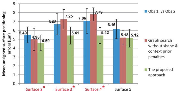
Unsigned surface positioning errors observed in 28 volumetric OCT images. Inter-observer variability is shown in blue, errors of the original graph search method with only hard constraints are shown in red [8], and errors of the proposed method are shown in green. For all four surfaces, the resulting errors are significantly smaller than the corresponding inter-observer variabilities (p < 0.001). Compared with the original graph search method, our method showed a significant improvement for surfaces 2, 3, and 4 (p < 0.05).

B. Qualitative Results

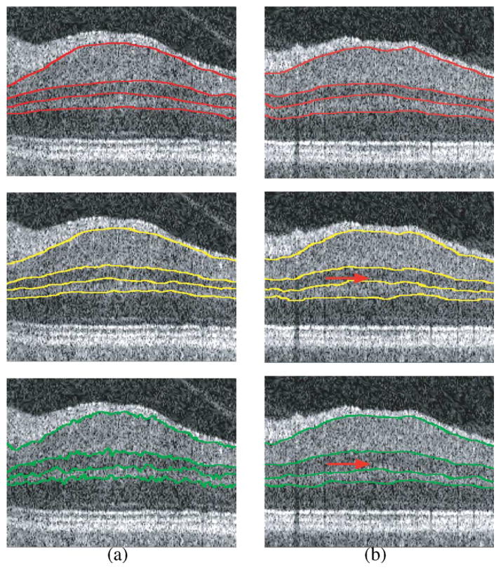
Qualitatively, the proposed algorithm produced very good segmentations. Fig. 9 shows the illustrative results of the proposed algorithm in comparison with the traditional graph search method using only hard constraints on one 2-D slice from the 3-D volume. Fig. 10(a) and (b) shows the contribution of the improvement made by the shape-prior penalties and context-prior penalties, respectively. In general, shape-prior penalties provide a better shape control, which leads to a more accurate and smoother segmentation. The context information helps to maintain the consistency of the layer thickness and avoid possible overlapping between adjacent surfaces.

Fig. 9.

Intraretinal layer segmentation in 3-D OCT images. (a) A 2-D slice from 3-D retinal OCT dataset. (b) Seven manually labeled surfaces (1–7). (c) Segmentation achieved using the former graph searching approach with only hard constraints—surfaces 2, 3, 4, 5. (d) Segmentation achieved using the proposed algorithm with shape and context prior penalties.

Fig. 10.

Improvements of segmentation contributed by (a) shape-prior penalties and (b) context prior penalties. The first row shows two slices of OCT images with manual segmentation. Segmentation results of two slices with both shape and context prior penalties are shown in the second row. The third row illustrates results (a) using context-prior penalties only (no shape-prior penalties) and (b) using shape-prior penalties only (no context-prior penalties).

VII. Discussion

A. Method Properties and Novelty

A novel approach for segmentation of multiple surfaces with both shape and context prior information was proposed. Our method advances the graph-based image segmentation in several important ways. First, the proposed energy function incorporates both shape prior and context prior information through a set of convex functions. Second, this approach allows simultaneous segmentation of multiple objects. Third, our method guarantees global optimality. To the best of our knowledge, this is the first method that fulfills these three aims at the same time. Here we list major novelty between our method and other state of the art segmentation approaches as follows.

1) Soft Constraints Versus Hard Constraints

The previous graph-search framework in [8] only allows the incorporation of hard shape constraints and hard context constraints. All shape changes or surface distances within the hard constraints are treated equally, which fails to fully make use of prior information. Instead, the proposed method allows the incorporation of “soft constraints,” which encourages certain shape change or surface distance value by penalizing the value less than other possible values within the hard constraints. It can be enforced by introducing additional shape-prior penalty term and context-prior penalty term in the energy through arc-weighted graph construction. Our method allows the incorporation of a wider spectrum of prior shape and context information.

2) Global Optimality Versus Local Optimality

Active contour and level set based methods also allow the incorporation of shape-prior information [34], [35]. A richer shape model can be encoded using nonconvex energies and can be solved using iterative based approach with a local optimal solution. In [36], Mishra et al. employed an active contour-based approach for retinal layer segmentation. The initial contours are computed using dynamic programming and then refined by adaptive kernel-based optimization. In [37], [38], an active contour method developed from the Chan–Vese’s model was adapted for intra-retinal layer segmentation. A circular shape prior was employed to model the boundary of the retinal layers. The major advantage of the proposed method to those methods is that our approach has a globally optimal guarantee, which ensures that the segmented results will not be trapped by local minima. In addition, it is nontrivial to apply active contour or level set based methods for simultaneous segmentation of multiple surfaces with the context constraints between neighboring surfaces.

3) Local Shape Information Versus Global Shape Information

The proposed method only incorporates local shape prior information, while many attempts have been made to incorporate global shape information, e.g., [39], [22], [26]. In [40], a novel probabilistic method was presented for intraretinal layer segmentation, which combines both local appearance information and a global shape information. We agree that the incorporation of global information helps to provide a better global shape control. However, it may lack local accuracy to deal with pathological data with large variations to the shape model in medical imaging. In addition, it is nontrivial to encode the context constraints for multiple objects segmentation together with a global shape control.

B. Time Complexity Analysis

Here, we compare the time complexity of the proposed method with the previous graph-search approach. Suppose the size of volumetric image is X × Y × Z. The target is to find λ terrain-like surfaces intersecting with z-axis. A four-neighboring system is defined for each column. Let T(n, m) denote the time for finding a maximum flow in an arc-weighted graph with O(n) nodes and O(m) arcs. For instance, by using Goldberg and Tarjan’s algorithm [41], T(n, m) = O(mn log(n²)/(m)). As described in [3], [4], the time complexity for the previous graph search framework is T(n′, m′) with n′ = |λXYZ| and m′ = |λXYZ|.

To incorporate shape-prior penalty term and the context-prior penalty term in proposed method, additional inter-column arcs and inter-surface arcs are introduced into the graph, respectively. Following the graph construction method in Section III-B, the total number of arcs m_s for shape-prior penalty is O(λXYZL_max), where L_max denotes the maximum hard shape constraint of all pairs of neighboring columns. Similarly, let H_max represents the maximum hard context constraint between adjacent surfaces in all columns. The total number of arcs m_c introduced for context-prior penalty is O(λXYZH_max). Note that no additional nodes are introduced. The time complexity of the proposed approach is T(n′, m″) with n′ = O(λXYZ) nodes and m″ = O(λXYZ(L_max + H_max)) arcs.

In practice, the average execution times of the proposed method as well as the previous approach are summarized in Table II. Basically, our method runs about 10 times slower compared with the previous approach due to the additional arcs carrying on the shape prior and context prior penalties. To reduce the execution time, the possible solutions include a parallel implementation of the maximum flow solver, for example, as described in [42]. In addition, a multi-scale approach can also be used. An approximate segmentation can be first performed using the previous method without the shape or context prior information to determine a rough region of interest for target surfaces. Then a final segmentation with both the shape and context prior information can be conducted in the reduced region of interest to achieve an accurate result. Further development of the proposed approach to reduce the running time will be our future work.

TABLE II.

Average Running Time for Simultaneous Segmentation of Surfaces 2–5

Method	Average running time (s)
Previous Graph Search	781
Shape Priors Only	3437
Context Priors Only	3314
Shape & Context Priors	7906

C. Extension to the Segmentation of Arbitrarily-Irregular Surfaces

The proposed framework can be directly extended to the segmentation of arbitrarily-irregular meshed surfaces. The basic idea can be presented as follows. An initial shape model is first built for each target object based on the prior information, which takes the form of triangulated meshes. The meshed model reflects the approximate topological structure of the target surfaces. A graph is then constructed based on this shape model. Multiple constraints (i.e., shape priors constraints, context prior constraints) are incorporated into the graph using the method proposed in Section III. Fig. 11(a) shows an example with two initial models constructed for the segmentation of the bladder and the prostate. For the bladder, the initial model is based on a pre-segmentation using the level-set method. For the prostate, the model is constructed from the mean prostate model learned from the training set, which is interactively fitted into an approximate bounding box for the prostate. The corresponding graph G_i(i = 1, 2) is built from the triangulated meshes of two initial models as follows. For each vertex v, a column of K nodes is created in G_i, denoted by p(v) [Fig. 11(b)]. The positions of nodes reflect the positions of the corresponding voxels in the image domain. The target surface S_i in the graph G_i is defined as the surface containing exactly one node in each column. To incorporate the context constraints, a “partially interacting area” is defined according to the distance between the two meshes, which indicates that the two target surfaces may mutually interact with each other in that area. The context relationships can be modeled in the following manner: for each column p(v₁) ∈ G₁ in the partially interacting area, there exists a corresponding column p(v₂) ∈ G₂ with the same position in the image space; the target surfaces S₁ and S₂ both cut those columns, as shown in Fig. 11(b). The context prior information is enforced in the area by adding inter-surface arcs between corresponding columns using the approach proposed in Section III-C. In our initial experiments, a nonoverlapping constraint is enforced, which requires that the distance between surfaces of the bladder and the prostate is at least 1, which avoids intersection of two surfaces.

Fig. 11.

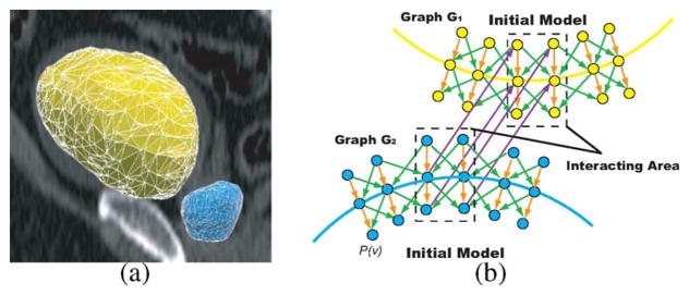
Segmentation of the prostate and bladder. (a) Triangular meshes for the bladder (yellow) and the prostate (blue) based on initial models. (b) Corresponding graph construction. An example 2-D slice is presented. p(v) represents the column with respect to the vertex v on the mesh. Dots represent nodes n_i ∈ G_i. Two sub-graphs G₁ and G₂ are constructed for the segmentation of the bladder and the prostate, respectively. Note that in the region of interaction (dashed box), a corresponding column in G₂ exists for each column in G₁ with the same position. The inter-surface arcs (purple) between corresponding columns enforce the surface context constraints in the interacting region.

Example results in three views are displayed in Fig. 12(a)–(d) and the 3-D representation is shown in Fig. 12(f), the proposed algorithm produces a very good delineation of both the bladder and the prostate in the 3-D space. While the shape prior constraints keep the original topological structure of the target organs, no overlap of the bladder and the prostate occur due to the enforcement of the context constraints.

Fig. 12.

Simultaneous segmentation of the bladder (yellow) and the prostate (blue) in 3-D CT images using the graph-search approach with shape and context priors. (a), (b) Transverse views. (c) Sagittal view. (d) Coronal view. (e) 3-D representation of the segmentation result.

D. Extension to N-D Surface Segmentation

The proposed method can be extended to N-D by constructing a geometric graph G = (N, A) in the N-D space (n ≥ 3) as follows. Given any undirected base graph G_B = (N_B, A_B) embedded in the (N − 1)-D space, a column of K nodes is built for each node n_i ∈ N_B denoted by p_i. If arc (n_i, n_j) ∈ N_B, we say that Columns p_i and p_j are adjacent. The target N-D “surface” is defined as the surface contains exactly one node in each column. To segment λ surfaces in the N-D space, the directed graph G consists of λ subgraphs, each of which is constructed from the (N − 1)-D based graph. Based on this definition, we can use exactly the same way described in Section III-C to incorporate both the shape and context prior information by adding weighted inter-column arcs and inter-surface arcs in the graph G. The optimal surfaces can be found by solving a maximum-flow problem in N-D. The possible applications include 4-D object segmentation with object motion over time, and co-segmentation of objects in multi-modality images.

E. Limitations

While the proposed framework can be easily applied to a number of image segmentation tasks, it also has several limitations. First, a set of convex functions is employed to enforce the shape prior and the context prior penalties. If the distribution of the prior shape information or the prior context information cannot be represented by a convex function set, encoding them into our framework may lead to a computationally intractable problem. Also, our current framework only enforces the local prior information, e.g., local shape constraints between neighboring columns. Encoding both local priors and global constraints is a challenging task. Some attempts have been made in [43] and [44], where the graph search framework is combined with the active shape model to provide a better global shape control. Furthermore, it is nontrivial for our method to deal with the regions of complex topology without an initial shape model, which needs to contain the basic topological information about the region’s surface. The initial model allows us to transform the problem of segmenting irregular surfaces into the segmentation of terrain-like surfaces. Note that if the target surfaces are already terrain-like surfaces, no initial model is required.

VIII. Conclusion

We presented a general framework for simultaneous segmentation of multiple surfaces, in which the prior shape and context information was incorporated into the energy function through a set of convex functions. An arc-weighted graph representation was employed and the optimal solution achieved by solving a maximum flow problem in a low order polynomial time. The proposed algorithm was validated in 28 datasets depicting human retina in OCT images. We have also demonstrated the applicability of our method to prostate-bladder segmentation. The results clearly demonstrated the applicability and improved performance of the proposed approach.

References

- 1.Freedman D, Radke R, Zhang T, Jeong Y, Lovelock D, Chen G. Model-based segmentation of medical imagery by matching distributions. IEEE Trans Med Imag. 2005 Mar;24(3):281–292. doi: 10.1109/tmi.2004.841228. [DOI] [PubMed] [Google Scholar]
- 2.Vu N, Manjunath B. Shape prior segmentation of multiple objects with graph cuts. Proc. IEEE Int. Conf. Comput. Vis. Pattern Recognit; Jun. 2008,; pp. 1–8. [Google Scholar]
- 3.Wu X, Chen DZ. Optimal net surface problems with applications. Proc. 29th Int. Colloq. Automata, Lang. Programm; 2002; pp. 1029–1042. [Google Scholar]
- 4.Li K, Wu X, Chen DZ, Sonka M. Optimal surface segmentation in volumetric images—A graph-theoretic approach. IEEE Trans Pattern Anal Mach Intell. 2006 Jan;28(1):119–134. doi: 10.1109/TPAMI.2006.19. [DOI] [PMC free article] [PubMed] [Google Scholar]
- 5.Yin Y, Zhang X, Williams R, Wu X, Anderson D, Sonka M. LOGISMOS—Layered optimal graph image segmentation of multiple objects and surfaces: Cartilage segmentation in the knee joints. IEEE Trans Med Imag. 2010 Feb;29(2):2023–2037. doi: 10.1109/TMI.2010.2058861. [DOI] [PMC free article] [PubMed] [Google Scholar]
- 6.Heimann T, Munzing S, Meinzer HP, Wolf I. A shape-guided deformable model with evolutionary algorithm initialization for 3D soft tissue segmentation. Proc. Biennial Int. Conf. Inf. Process. Med. Imag. (IPMI); 2007; pp. 566–577. [DOI] [PubMed] [Google Scholar]
- 7.Zhao F, Zhang H, Wahle A, Thomas M, Stolpen A, Scholz T, Sonka M. Congenital aortic disease: 4D magnetic resonance segmentation and quantitative analysis. Med Image Anal. 2009;13(3):483–493. doi: 10.1016/j.media.2009.02.005. [DOI] [PMC free article] [PubMed] [Google Scholar]
- 8.Garvin M, Abramoff MD, Wu X, Russell SR, Burns TL, Sonka M. Automated 3-D intraretinal layer segmentation of macular spectral-domain optical coherence tomography images. IEEE Trans Med Imag. 2009 Sep;28(9):1436–1447. doi: 10.1109/TMI.2009.2016958. [DOI] [PMC free article] [PubMed] [Google Scholar]
- 9.Xu X, Niemeijer M, Song Q, Sonka M, Garvin M, Reinhardt JM, Abramoff MD. Vessel boundary delineation on fundus images using graph-based approach. IEEE Trans Med Imag. 2011 Jun;30(6):1184–1191. doi: 10.1109/TMI.2010.2103566. [DOI] [PMC free article] [PubMed] [Google Scholar]
- 10.Song Q, Wu X, Liu Y, Haeker M, Sonka M. Simultaneous searching of globally optimal interacting surfaces with shape priors. Proc. IEEE Int. Conf. Comput. Vis. Pattern Recognit; 2010; pp. 2879–2886. [Google Scholar]
- 11.Kass M, Witkin A, Terzopoulos D. Snakes: Active contour models. Int J Comput Vis. 1988;1(4):321–331. [Google Scholar]
- 12.Caselles V, Kimmel R, Sapiro G. Geodesic active contours. Int J Comput Vis. 1997;22:61–97. [Google Scholar]
- 13.Osher S, Sethian JA. Fronts propagating with curvature dependent speed: Algorithms based on Hamilton-Jacobi formulations. J Computat Phys. 1988;79:12–49. [Google Scholar]
- 14.Sethian JA. Level Set Methods and Fast Marching Methods. Cambridge, U.K: Cambridge Univ. Press; 1999. [Google Scholar]
- 15.Rousson M, Paragios N, Deriche R. Implicit active shape models for 3d segmentation in MRI imaging. Proc. Int. Conf. Med. Image Comput. Computer-Assist. Intervent; 2004; pp. 209–216. [Google Scholar]
- 16.Cremers D. Dynamical statistical shape priors for level set based tracking. IEEE Trans Pattern Anal Mach Intell. 2006 Aug;28(8):1262–1273. doi: 10.1109/TPAMI.2006.161. [DOI] [PubMed] [Google Scholar]
- 17.Rousson M, Paragios N. Priorknowledge, levelset representation & visual grouping. Int J Comput Vis. 2008;76(3):231–243. [Google Scholar]
- 18.Chan T, Esedoglu S, Nikolova M. Algorithms for finding global minimizers of image segmentation and denoising models. SIAM J Appl Math. 2006;66(5):1632–1648. [Google Scholar]
- 19.Pock T, Schoenemann T, Graber G, Bischof H, Cremers D. A convex formulation of continuous multi-label problems. Proc. Eur. Conf. Comput. Vis; 2008; pp. 792–805. [Google Scholar]
- 20.Lellmann J, Becker F, Schnorr C. Convex optimization for multi-class image labeling with a novel family of total variation-based regularizers. Proc. IEEE Int. Conf. Comput. Vis; 2009; pp. 646–653. [Google Scholar]
- 21.Pock T, Chambolle A, Cremers D, Bischof H. A convex relaxation approach for computing minimal partitions. Proc. IEEE Int. Conf. Comput. Vis. Pattern Recognit; 2009; pp. 810–817. [Google Scholar]
- 22.Cremers D, Schmidt F, Barthel F. Shape priors in variational image segmentation: Convexity, Lipschitz continuity and globally optimal solutions. Proc. IEEE Int. Conf. Comput. Vis. Pattern Recognit; 2008; pp. 1–6. [Google Scholar]
- 23.Andrews S, McIntosh C, Hamarneh G. Convex multi-region probabilistic segmentation with shape prior in the isometric logratio transformation space. Proc. IEEE Int. Conf. Comput. Vis; 2011; pp. 2096–2103. [Google Scholar]
- 24.Felzenszwalb P, Huttenlocher D. Efficient graph-based image segmentation. Int J Comput Vis. 2004;59(2):167–181. [Google Scholar]
- 25.Boykov Y, Funka-Lea G. Graph cuts and efficient N-D image segmentation. Int J Comput Vis. 2006;70(2):109–131. [Google Scholar]
- 26.Felzenszwalb P. Representation and detection of deformable shapes. IEEE Trans Pattern Anal Mach Intell. 2005 Feb;27(2):208–220. doi: 10.1109/tpami.2005.35. [DOI] [PubMed] [Google Scholar]
- 27.Schoenemann T, Cremers D. Globally optimal image segmentation with an elastic shape prior. Proc. IEEE Int. Conf. Comput. Vis; 2007; pp. 1–6. [Google Scholar]
- 28.Freedman D, Zhang T. Interactive graph cut based segmentation with shape priors. Proc. IEEE Int. Conf. Comput. Vis. Pattern Recognit; 2005; pp. 755–762. [Google Scholar]
- 29.Malcolm J, Rathi Y, Tannenbaum A. Graph cut segmentation with nonlinear shape priors. Proc. IEEE Int. Conf. Image Process; 2007; pp. 365–368. [Google Scholar]
- 30.Delong A, Boykov Y. Globally optimal segmentation of multiregion objects. Proc. IEEE Int. Conf. Comput. Vis; 2009; pp. 285–292. [Google Scholar]
- 31.Ishikawa H. Exact optimization for Markov random fields with convex priors. IEEE Trans Pattern Anal Mach Intell. 2003 Oct;25(10):1333–1336. [Google Scholar]
- 32.Hochbaum DS. An efficient algorithm for image segmentation, Markov random fields and related problems. J ACM. 2001;48:686–701. [Google Scholar]
- 33.Garvin M, Wu X, Abramoff M, Kardon R, Sonka M. Incorporation of regional information in optimal 3-D graph search with application for intraretinal layer segmentation of optical coherence tomograph images. Proc. Biennial Int. Conf. Inf. Process. Med. Imag. (IPMI); 2007; pp. 607–618. [DOI] [PubMed] [Google Scholar]
- 34.Chen Y, Tagare HD, Thiruvenkadam S, Huang F, Wilson D, Gopinath KS, Briggs RW, Geiser EA. Using prior shapes in geometric active contours in a variational framework. Int J Comput Vis. 2002;50(3):315–328. [Google Scholar]
- 35.Chan T, Zhu W. Level set based shape prior segmentation. Proc. IEEE Int. Conf. Comput. Vis. Pattern Recognit; 2005; pp. 1164–1170. [Google Scholar]
- 36.Mishra A, Wong A, Bizheva K, Clausi DA. Intra-retinal layer segmentation in optical coherence tomography images. Opt Exp. 2009;17(26):23719–23728. doi: 10.1364/OE.17.023719. [DOI] [PubMed] [Google Scholar]
- 37.Yazdanpanah A, Hamarneh G, Smith B, Sarunic M. Intraretinal layer segmentation in optical coherence tomography using an active contour approach. Proc. Int. Conf. Med. Image Comput. Computer-Assist. Intervent; 2009; pp. 649–656. [DOI] [PubMed] [Google Scholar]
- 38.Yazdanpanah A, Hamarneh G, Smith BR, Sarunic MV. Segmentation of intra-retinal layers from optical coherence tomography images using an active contour approach. IEEE Trans Med Imag. 2011 Feb;30(2):484–496. doi: 10.1109/TMI.2010.2087390. [DOI] [PubMed] [Google Scholar]
- 39.Cootes TF, Taylor CJ, Cooper DH, Graham J. Active shape models—Their training and application. Comput Vis Image Understand. 1995;61(1):38–59. [Google Scholar]
- 40.Rathke F, Schmidt S, Schnörr C. Order preserving and shape prior constrained intra-retinal layer segmentation in optical coherence tomography. Proc. Int. Conf. Med. Image Comput. Computer-Assist. Intervent; 2011; pp. 370–377. [DOI] [PubMed] [Google Scholar]
- 41.Goldberg A, Tarjan R. A new approach to the maximum-flow problem. J Assoc Comput Mach. 1988;35(4):921–940. [Google Scholar]
- 42.Delong A, Boykov Y. A scalable graph-cut algorithm for ND grids. Proc. IEEE Int. Conf. Comput. Vis. Pattern Recognit; 2008; pp. 1–8. [Google Scholar]
- 43.Sun S, Bauer C, Beichel R. Automated 3D segmentation of lungs with lung cancer in CT data using a novel robust active shape model approach. IEEE Trans Med Imag. 2012 Feb;31(2):449–460. doi: 10.1109/TMI.2011.2171357. [DOI] [PMC free article] [PubMed] [Google Scholar]
- 44.Zhang H, Abiose A, Campbell D, Sonka M, Martins J, Wahle A. Left-ventricle segmentation in real-time 3D echocardiography using a hybrid active shape model and optimal graph search approach. Proc. SPIE Med. Imag.: Image Process; 2010; pp. 76261C-1–12. [Google Scholar]