A discrete-time multiple event process survival mixture (MEPSUM) model

Abstract

Traditional survival analysis was developed to investigate the occurrence and timing of a single event, but researchers have recently begun to ask questions about the order and timing of multiple events. A multiple event process survival mixture model is developed here to analyze non-repeatable events measured in discrete-time that may occur at the same point in time. Building on both traditional univariate survival analysis and univariate survival mixture analysis, the model approximates the underlying multivariate distribution of hazard functions via a discrete-point finite mixture in which the mixing components represent prototypical patterns of event occurrence. The model is applied in an empirical analysis concerning transitions to adulthood, where the events under study include parenthood, marriage, beginning full-time work, and obtaining a college degree. Promising opportunities, as well as possible limitations of the model and future directions for research are discussed.

Survival analysis is a useful tool for understanding both the occurrence and the timing of events. While survival analysis was originally developed to investigate the human lifetime, it is equally applicable to questions regarding the occurrence of any type of event, and there are numerous applications in the social and behavioral sciences. For example, clinical psychologists investigating the occurrence of affective illnesses or therapy termination benefit from the survival analysis framework (e.g. Corning & Malofeeva, 2004), as do developmental researchers who investigate the transition from one developmental stage to another (e.g. Ha, Kimpo, & Sackett, 1997), and researchers following students’ entrance and exit from school (e.g. Bowers, 2010).

Event history data is rather unique in that it aims to determine both if and when an event occurs, yet there are often individuals who do not experience the event within the time frame of the study. Traditional linear and logistic regression techniques are not suited for this kind of missing data problem, termed censoring. For censored individuals, it is unknown when they will experience the event, or in some cases whether they will experience the event at all. Survival analysis techniques were formulated to analyze this type of data (Singer & Willet, 2003; Lee & Wang, 2003). The basic statistical concepts of survival analysis depend on whether the time variable measuring the state of the event is continuous or discrete. Continuous-time survival methods assume event times can be measured exactly – thus there should be no “ties” in the dataset where two or more people have the same event time. While it may be logical to think of time as a continuous variable, this assumption is often unrealistic in practice. This is especially true for data collected in the social and behavioral sciences, as researchers frequently ask for the year or age of an event rather than the exact date. Also, events can sometimes only occur at discrete points in time (e.g. number of therapy sessions before dropout). In addition, discrete-time methods can be used to approximate the results of a continuous-time survival analysis (Vermunt, 1997), and are conceptually and computationally simpler. As such, the remainder of the paper focuses on models where time is measured on a discrete scale.

Moving beyond traditional survival analysis, researchers have recently begun to ask questions about the order and timing of multiple events. Multivariate survival models, such as recurrent event models, parallel data models, and competing risks models, relax the standard requirement that all time variables are univariate and independent (see Hougaard, 2000). For example, Gabadinho et al. (2011) discuss a technique called trajectory mining and provide an R package for analyzing sequences of events such as career or family trajectories. While there has been great progress on the analysis of multivariate event history data using these kinds of models, there is a demonstrated need for new analytic methods in investigating the order and timing of different non-repeatable events which may occur at the same point in time and do not necessarily occur in a sequential manner. Many researchers investigating several such events have resorted to completing a separate survival analysis for each event, and have not directly examined the interdependence of the events. For example, Schwartz et al. (2010) investigated how positive youth development influenced tobacco, alcohol, illicit drug, and sex initiation by conducting four separate survival analyses. Similarly, Scott et al. (2010) examined the influence of gender and marital status on the first onset of mood, anxiety, and substance use disorders by conducting several survival analyses. While analyzing each event separately can be useful, it gives no insight on how the events are related to each other.

Vermunt (1997) provides a general log-linear framework for modeling event history data with mixture models and builds off the work of Mare (1994) who presented a bivariate survival mixture model for analyzing event times of clustered observations, for example siblings or couples. Vermunt also suggests that multiple processes measured in discrete-time may be modeled by specifying one of the events as the dependent variable and treating others as time-varying covariates. However, researchers must rotate the dependent variable and run multiple models in order to investigate the reciprocal relationships. Malone et al. (2010) used a different approach for discrete-time data called dual-process discrete-time survival analysis, which expands on associative latent transition analysis (Bray, Lanza, & Collins, 2010). This approach models two time-to-event processes concurrently by linking the processes to each other, similar to a cross-lagged panel design. They used the model to test the gateway drug hypothesis by using a highly constrained latent transition matrix to model and test the cross-links between time to illicit drug use and time to licit drug use.

In addressing the need for a model which can be expanded for more than two events and which is developed specifically for the situation where the events may occur at the same point in time for an individual, we have two main objectives. The first objective of this paper is to introduce a discrete-time Multiple Event Process SUrvival Mixture (MEPSUM) model, a latent variable approach to analyzing the interdependencies between multiple non-repeatable events which are measured in discrete-time. The approach is mathematically a generalization of single-event discrete-time survival mixture analysis (Muthén & Masyn, 2005), but is conceptually different in some ways and has several advantages in addition to incorporating multiple events. The second objective of the paper is to demonstrate the usefulness of the model through an empirical analysis, which was the motivation behind this work. The analysis concerns the timing and occurrence of four different markers of adulthood: parenthood, marriage, full-time work, and obtaining a college degree from individuals in the National Longitudinal Study of Adolescent Health (Add Health).

The remainder of the introduction is organized into four sections. In the first section, the motivating example mentioned above is introduced. The second section outlines the basic concepts of traditional univariate discrete-time survival analysis, in order to introduce the discrete-time multiple event process survival mixture model in the third section. The fourth section regards model description and evaluation tools, and these are illustrated in the empirical analysis concerning transitions to adulthood that follows.

Motivating Example

Researchers have long established that the events experienced by individuals over their lifetimes are interdependent. For example, individuals may make decisions on whether they would like to continue their education based on their family status, such as whether they are married and have children (Marini, 1984). More broadly, life course research is guided by the notion that an individual’s development involves the order and timing of multiple social roles over time where the meaning of a given social role is dependent upon the presence or absence of other roles (Elder, 1985). Yet instead of investigating the multidimensional nature of the life course, researchers typically focus on one aspect of the life course, such as timing of an individual’s first child; then they examine this event in isolation from other life course events using traditional methods such as linear and logit regression and univariate event history models. However, as the significance of a role depends on the role configuration, dissecting the life course in such a way limits our understanding of the life course as a dynamic phenomenon (Macmillan & Eliason, 2003).

In aiming to understand the dynamic, multidimensional nature of the life course, the MEPSUM model is applied to the timing of four different transitions into adulthood. The purpose of this analysis is both to demonstrate the model’s applicability to life course theory and to build on prior research by examining the latent classes which reveal pathways to adulthood, or patterns of the events over time (Shanahan, 2000; Shanahan, Miech, & Elder, 1998). The life course pathways found from this model are prototypical and are not expected to be the only pathways through the life course, but they provide a glimpse at the underlying multivariate distribution of pathways, of which there are likely thousands of possibilities. Additionally, this example is useful in examining the ability of the model to detect differences in pathways taken by different social groups. By examining the multidimensional nature of the life course, the model gives insight into the possible mechanisms leading to differences in life course pathways. It is possible that a covariate influences the multivariate distribution of the risk of multiple events in a way that does not lend itself to be discovered by traditional methods that analyze events one at a time. For example, a covariate might increase the risk of transitioning into family roles for those who do not pursue college education but decrease the risk of transitioning into family roles for those pursuing a college education. Thus, the added complexity of the MEPSUM model has potential to increase our understanding of multiple transitions over time.

Discrete-Time Survival Analysis

Before introducing the MEPSUM model in more detail, it is useful to outline the basic concepts of univariate survival analysis. Let T denote the event time, and j the discrete time point, with j =1, 2, …, J. There are many methods of characterizing the probability distribution of the event time. The simplest way is to define the probability of experiencing an event at a specific time period:

$$f_j=P(T=j)$$ (1)

Another option is the survival function, which is defined as the probability that an individual survives longer than j and is denoted S_j:

$$S_j=P(T>j)=1-\sum _{m=1}^j{f}_m$$ (2)

with S_j = 1 at j = 0. The survival function is often used to find descriptive measures of the event history, such as the median lifetime: an estimate of the time period when the event has occurred for fifty percent of the population. Such descriptive measures are important when there is censoring, as measures such as the sample mean will not be useful in describing the center of the distribution when the event time is not known for all individuals.

An equally useful function known as the lifetime distribution function defines the probability that an individual has experienced the event by time j:

$$D_j=P(T\le j)=1-S_j=\sum _{m=1}^j{f}_m$$ (3)

Importantly, the number of individuals who experienced the event at T = j is unknown if there are censored individuals. Thus, neither the survival function nor lifetime distribution function can be directly estimated, as f_j is unknown.

The hazard probability h is the first function that can be estimated with both censored and uncensored individuals. It is the conditional probability that the event occurs at j given that it did not occur prior to j:

$$h_j=P(T=j\mid T\ge j)=P(T=j\mid T>j-1)=\frac{P(T=j)}{P(T>j-1)}$$ (4)

The hazard for time j is estimated as the number of events that occur at j over the number of individuals in the risk set. It thus tells us the unique risk of event occurrence for each time period among those eligible to experience the event, which is exactly what we want to know: whether and when events occur. It is estimable with censored individuals as it is a conditional probability computed only using individuals eligible to experience the event, and can be computed for every time period when event occurrence is recorded. Under an assumption of noninformative censoring, we can assume the estimated hazard function applies to the entire population, as all non-censored individuals at each time period are representative of all individuals who would have remained in the study if censoring had not occurred.

It is important to note that the hazard function can be re-written in terms of f_j and S_j:

$$h_j=\frac{f_j}{S_{j-1}}=1-\frac{S_j}{S_{j-1}}$$ (5)

This relationship is useful in obtaining an estimate of the survival function when there are censored individuals, as Equation (4) can be rearranged to show:

$$S_j=\left[S_{j-1}\right]\left[1-h_j\right]$$ (6)

Given this relationship and the fact the survival function is equal to one at j = 0 (no individual experienced an event before the beginning of the time variable) this leads to the idea that the survival probability at time period j is the product of the hazard probabilities for each of the earlier time points:

$$S_j=\prod _{m=1}^j(1-h_m)$$ (7)

The lifetime distribution function can similarly be estimated indirectly from the hazard probabilities, or by the simple relationship between D_j and S_j given in Equation (3).

The next step of a survival analysis is to model the probability distribution and add covariates to the model to examine their influence. In line with Singer and Willet (1993), a logit link function will be used for the remainder of the paper, but other link functions such as the complementary log-log link are equally applicable to all of the survival methods discussed hereafter. The unstructured hazard function at time j without covariates is then given by:

$$\mathit{logit}\left(h_j\right)=\mathit{ln}\left(\frac{h_j}{1-h_j}\right)={\alpha }_j$$ (8)

where α_j is the intercept parameter for time j. This model represents the log-odds of event occurrence as a function of the time period only.

There are almost countless ways to expand on the simple unstructured discrete-time hazard model discussed here (e.g. Singer & Willet, 2003; Allison, 1999). For example, instead of allowing an intercept for each time period which places no constraints on the shape of the hazard, it is possible to have a polynomial representation of time. When the number of time periods is large or some time periods have very small risk sets, it can be advantageous to fit a more parsimonious model. For simplicity purposes, the remainder of the paper will focus on the unstructured hazard with a logit link function, but the equations that follow can be easily generalized to alternative functions as mentioned above. Finally, it is also possible for both time invariant as well as time varying predictors to be added to the model. Traditional univariate survival analysis thus provides an important conceptual and analytic framework from which to evaluate if and when one non-repeatable event occurs.

Model for Multiple Events

A discrete-time Multiple Event Process SUrvival Mixture (MEPSUM) model is now developed to examine multiple non-repeatable events. A finite mixture is used to approximate the multivariate hazard distribution of the events (consistent with Heckman & Singer, 1984; Nagin, 1999; and Nagin & Land, 1993). The components of the mixture, or latent classes, represent local regions within the multivariate distribution, providing a succinct summary of individual differences in patterns of event occurrence over time. In other words, the model provides a non-parametric way to capture associations between events through the identification of latent classes of individuals with similar risk, or hazard, for multiple events over time. Although it may be tempting to interpret these classes literally (i.e., as qualitatively distinct population subgroups), we regard it as more likely that the underlying multivariate hazard distribution is in fact continuous in nature. Thus, the classes merely provide a statistically expedient way to represent this distribution in a simple, mathematically tractable form that captures evidence in the data of how the events are related to each other. The model is easily expanded beyond two events and enables researchers who aim to analyze multiple events to utilize all individuals in their dataset, including those with censored event times.

Substantively, the model allows researchers to understand both the order and timing of the events through examination of the hazard functions both within each latent class and across latent classes. Additionally, both the survival function and lifetime distribution function for each event can be compared across latent classes, as these functions may be estimated indirectly from the fitted hazard functions through Equation (3) and Equation (7). Predictors can be incorporated into the model to investigate potential influences on the risk for multiple events over time.

Suppose the event history variable y_ipj for person i represents whether a process of type p (p = 1, 2, …, P) occurs at time period j (j = 1, 2, …, J_ip) and the response vector y_i holds the event history variable across all time periods and processes [(y_i11, …, y_i1Ji1), (y_i21, …, y_i2Ji2),…,(y_iP1,…,y_iPJiP)]’. The total number of time points under study for event process p is represented by J_p. Note the flexibility of the model in that the number of time periods studied can vary between processes, the width of the time periods can vary within processes, and the length of the vector can vary between individuals.

Let y_ipj = 0 if the non-repeatable event for process p did not occur for individual i at that time period or earlier and y_ipj = 1 if the event occurred at that time period. By framing the data in this way, individuals only contribute data at j for process p when they are in the risk set at j for process p (i.e., when the event has not yet occurred), similar to a standard univariate survival analysis. For example, consider two event processes (e.g. onset of depression and onset of an anxiety disorder), which are both measured annually from 10 years old to 14 years old. An individual who responds at age 15 with no history of either disorder would have the event history ( 0 0 0 0 0 ) for each process. In contrast, consider an individual who is measured at age 13 who was diagnosed with an anxiety disorder at age 11. The event history for depression would only include data from ages 10 to 13 ( 0 0 0 0 ), and the event history for anxiety would only include data from ages 10 to 11 ( 0 1 ). Individuals with an unknown event time are said to be censored, and the model assumes that this data is missing at random. This assumption of noninformative censoring is important, for we can then assume all non-censored individuals at each time period are representative of all individuals who would have remained in the study if censoring had not occurred. This allows generalization to the entire data set and thus the original population.

The risk of event occurrence (y_ipj = 1), or the conditional probability of event occurrence given it did not occur before, for event process p in time period j within latent class k is represented by h_pjk. Within latent class k, h_pjk is modeled using a simple unstructured discrete-time hazard function with time-specific intercept α_pjk:

$$\mathit{logit}\left(h_{\mathit{pjk}}\right)={\alpha }_{\mathit{pjk}}$$ (9)

A more complex version of the model could include both effects of time-invariant and time-varying covariates directly in the hazard function above, which would create direct effects of the covariates on the hazard functions. Note that adding such direct effects substantially increases the complexity of the model and can create difficulties for interpretation. If necessary, direct effects should initially be entered as class-invariant, as any parameter that varies over latent classes provides information to identify and discriminate the latent classes (Petras & Masyn, 2010).

It is also possible to structure the hazard function, such as imposing a quadratic form. However, caution is needed before imposing such a structure. Basing this structure on the shape of the total-sample estimated hazard function may be incorrect, as it is possible that this shape will not hold within or across latent classes, as will be seen in the empirical example that follows. Additionally, it is possible that different events have different parametric forms. Results from the MEPSUM model with unstructured hazard functions can serve as a guide to possible parametric forms of the hazard functions.

The model assumes that all marginal associations among the hazard functions are captured though between-class differences, so that the observed hazard indicators are independent within latent class. This implies the probability of a specific response vector within a given latent class k can be obtained by simply multiplying the probability of all of the responses:

$$P({\mathbf{y}}_i\mid C_i=k)=\prod _{p=1}^P\prod _{j=1}^{\mathit{Jip}}\left({h_{\mathit{pijk}}}^{y_{\mathit{ipj}}}{(1-h_{\mathit{pijk}})}^{(1-y_{\mathit{ipj}})}\right)$$ (10)

The indicator variable y_ipj functions as a device for selecting the appropriate probability by which to multiply. When the event occurs (y_ipj = 1) for process p at time period j, the model multiplies by h_pijk, versus event nonoccurrence for process p at time period j when the model multiplies by (1 - h_pijk).

The overall probability of response pattern y_i is a weighted average across all of the latent classes of the probability of being in latent class k given by π_ik and probability of y_i given latent class k as defined in Equation (10):

$$P\left({\mathbf{y}}_i\right)=\sum _{k=1}^K{\pi }_{\mathit{ik}}P({\mathbf{y}}_i\mid C_i=k)$$ (11)

where π_ik is modeled using standard multinomial logistic regression. With time-invariant predictors X_i, this is given by:

$${\pi }_{\mathit{ik}}=\frac{\exp ({\gamma }_{0K}+{\gamma }_K^{\prime }{\mathbf{X}}_i)}{\sum _{w=1}^K\exp ({\gamma }_{0w}+{\gamma }_w^{\prime }{\mathbf{X}}_i)}$$ (12)

where the last class is a reference class with γ_0K = 0 and ${\gamma }_K^{\prime }=0$, and ${\sum }_{k=1}^K{\pi }_{\mathit{ik}}=1$. This leaves us with the final equation for the probability of an event history response vector:

$$P\left({\mathbf{y}}_i\right)=\sum _{k=1}^K\left({\pi }_{\mathit{ik}}\prod _{p=1}^P\prod _{j=1}^{\mathit{Jip}}\left({h_{\mathit{pijk}}}^{y_{\mathit{ipj}}}{(1-h_{\mathit{pijk}})}^{(1-y_{\mathit{ipj}})}\right)\right)$$ (13)

and the likelihood function:

$$L=\prod _{i=1}^n\left[\sum _{k=1}^K\left({\pi }_{\mathit{ik}}\prod _{p=1}^P\prod _{j=1}^{\mathit{Jip}}\left({h_{\mathit{pijk}}}^{y_{\mathit{ipj}}}{(1-h_{\mathit{pijk}})}^{(1-y_{\mathit{ipj}})}\right)\right)\right]$$ (14)

which is used to find optimal parameter estimates. In large sample surveys, individuals are often drawn with unequal selection probabilities and the contribution of individual i may be weighted by a sample weight, which is often computed as the inverse probability of selection into the sample or through a function that also takes other features of the survey into account (Kish, 1965; Lohr, 2009).

The model may be fit using latent variable modeling software such as Mplus (Muthén & Muthén, 1998-2010) or Latent Gold (Vermunt & Magidson, 2005), which obtain maximum-likelihood model parameter estimates using an Expectation-Maximization (EM) algorithm. Researchers should be aware of an issue that commonly arises with modeling the probability of a binary outcome with a logit link: the logit is undefined if the probability is exactly zero or one. This could occur in time periods where there is no risk of event occurrence. To address this issue, Mplus implements default bounds on the logits of ±15, while Latent Gold utilizes a Bayesian approach, including a Dirichlet prior for the latent and conditional response probabilities that serves to smooth parameter values away from the boundary solution.¹ No matter what software program is selected, researchers should remain cognizant of the methods employed by the program to address this issue. It should also be noted that mixture models in general are susceptible to converge at local rather than global maxima. Multiple starting values should be used, and the convergence pattern should be monitored (McLachlan & Peel, 2000; Hipp & Bauer, 2006). Example data and code for fitting the model are given at www.unc.edu/~dbauer.

Importantly, the single event version of this model with unstructured hazard functions, presented by Muthén & Masyn (2005), is not identified without covariates, as there is not enough information in one event process for the model to differentiate latent classes. An unfortunate side effect is that the classes revealed from a single event mixture model are then necessarily dependent upon the covariates entered into the model and different sets of covariates may result in nontrivial differences in the formation of the latent classes. In contrast, a major benefit of the MEPSUM model for multiple events is that it can have positive degrees of freedom for multiple classes, even with unstructured hazard functions and in the absence of covariates. This is due to the fact that with multiple event processes, the observed variables are independent within event process, but are not independent across processes, which can result in positive degrees of freedom. The latent variable is thus able to capture interdependencies between the hazard functions of the different process through the addition of latent classes. Identification of the model without covariates thus allows investigation of the stability of the latent classes, through comparison of model results with and without covariates.

However, as in all models, empirical underidentification may still be a concern. When there is little dependence between event history indicators across processes, the resulting information matrix can be so empirically near non-positive definite that the software fails to reach a solution or results in boundary estimates.² Researchers should carefully monitor the estimation process and parameter values that are output, and start values may assist in the convergence process. In our limited experience applying the model to date, we have generally found the model is identified with at least three event processes, even with unstructured hazard functions and without covariates. One may draw insight from related literature on latent class analysis and growth mixture modeling to formulate an appropriate model building strategy (e.g. Petras & Masyn, 2010; Bandeen-Roche, Miglioretti, Zeger, & Rathouz, 1997; Collins & Lanza, 2010; Vermunt & Magidson, 2002).

Class Enumeration and Model Evaluation

Models with different number of latent classes may be evaluated and compared using information criteria such as Akaike information criterion (AIC), Bayesian information criterion (BIC), and sample-size adjusted BIC (SABIC) as well as classification indices measuring the degree of uncertainty of classification or separation of the clusters (Akaike, 1974; Schwarz, 1978; Bozdogan, 1987; Fraley, & Raftery, 1998; Celeux, Biernacki, & Govaert, 1997; Vermunt & Magidson, 2002). The Lo-Mendell-Rubin likelihood ratio test and parametric bootstrap likelihood ratio test are other common approaches to selecting the number of classes and evaluating model fit (Lo, Mendell, & Rubin, 2001; McLachlan, & Peel, 2000; Nylund, Asparouhov, & Muthén, 2007). Researchers may also examine the results to determine whether a class is redundant or whether the probability of belonging to a class is very small, as parameter estimates in a low probability class may not be stable due to the small number of individuals contributing data to that class.

In evaluating model fit, a researcher cannot compare the estimated latent classes to observed subpopulations, since the classes are unobserved and inferred from the data. However, one model evaluation and selection tool is the ability to compare the sample observed functions with the marginal model implied functions weighting over latent classes. The aggregate model implied lifetime distribution function for process p is found by weighting the marginal within-class function by the probability of class membership ${\widehat{\pi }}_k$:

$${\widehat{D}}_{\mathit{pj}}=\sum _{k=1}^K{\widehat{\pi }}_k{\widehat{D}}_{\mathit{pjk}}$$ (15)

The standard residual lifetime distribution (SRD) can be then be computed across all event processes in order to evaluate the difference between the marginal population-level model implied functions and the sample observed functions. A smaller SRD implies closer fit between the sample observed lifetime distribution function and the model implied population-level function. With P event process, each with J_P events, this is given by:

$$\mathit{SRD}=\sqrt{\frac{\sum _{p=1}^P\sum _{j=1}^{J_p}{\left(D_{\mathit{pj}}-{\widehat{D}}_{\mathit{pj}}\right)}^2}{\sum _{p=1}^P{J}_p}}$$ (16)

where D_pj is the sample observed lifetime distribution function for process p.

Computing the model implied hazard functions weighting over latent classes is less straightforward, as the number of people eligible to experience the event in each class will decrease unevenly due to differential risk of event occurrence. Therefore, the population average hazard functions must be computed by weighting the marginal within-class hazard functions not only by the probability of event occurrence, but also by the number eligible to experience the event at time j within a latent class k. The number eligible to experience the event is equal to the survival probability at time j – 1, and the model implied hazard function weighting over latent classes is then given by:

$${\widehat{h}}_{\mathit{pj}}=\frac{\sum _{k=1}^K{\widehat{\pi }}_k{\widehat{S}}_{p,j-1,k}{\widehat{h}}_{\mathit{pjk}}}{\sum _{k=1}^K{\widehat{\pi }}_k{\widehat{S}}_{p,j-1,k}}$$ (17)

The standard residual hazard across all event processes is given by:

$$\mathit{SRH}=\sqrt{\frac{\sum _{p=1}^P\sum _{j=1}^{J_p}{\left(h_{\mathit{pj}}-{\widehat{h}}_{\mathit{pj}}\right)}^2}{\sum _{p=1}^P{J}_p}}$$ (18)

where h_pj is equal to the sample observed hazard function for process p. Again, this function is useful in determining the difference between the marginal population-level model implied functions and the sample observed functions. Ideally, SRH would be very close to 0, which is likely when the form of the hazard functions is left unstructured.

The model implied functions defined above may also be used in a descriptive manner to evaluate the overall effects of covariates, by first computing the predicted probabilities of class membership based on different levels of covariates, and then using those predicted probabilities to weight the within-class functions. These steps contrast with the functions given above in that the predicted probabilities are now computed conditional on the level of the covariates, e.g. ${\widehat{D}}_{\mathit{pjk}\mid X}$. With an appropriate sample size and categorical covariates, one can also stratify the sample in order to compute sample observed functions for specific levels of the covariates, and can then calculate standard residual lifetime distribution and standard residual hazard based on these functions. Resulting model implied functions allow one to evaluate overall differences in the risk for multiple events over time for different levels of a covariate, as will be illustrated in the example that follows.

Methods

The data for the empirical example come from Wave I and Wave IV of the National Longitudinal Study of Adolescent Health (Add Health; Harris et al., 2009). Add Health began in the 1994-1995 school year with a nationally representative sample of adolescents from 80 high schools and 52 middle schools in the United States selected with unequal probability of selection.³ The individuals were then followed from adolescence into adulthood through four in-home interviews. Parental interviews were also completed during the first wave. The last interview, Wave IV, was completed in 2008, when the majority of the sample was twenty-four to thirty-two years old. At each wave, information was gathered on respondents’ social, economic, psychological, and physical well-being. Wave IV in-home interviews were completed for 15,701 individuals.

Four role status variables were examined: marriage, college graduation, full-time work, and parenthood (Shanahan, 2000). For each age from 18-30, a binary variable for each status was created indicating whether the individual occupied the status for the first time at that age (coded 1), or had not occupied the status by that age (coded 0). Once the individual occupied one of the role statues, they no longer contributed data for the remaining ages for that status (coded as missing). To account for the fact that a small percentage of individuals occupied one of the roles before they were eighteen years old, the binary variable for age 18 will represent whether the individual occupied the status for the first time at age 18 or younger. In essence, this is structuring the first time period to be wider (from birth to age 18) than any of the other time periods, which all represent one year.

The role status variables were taken from the Wave IV Add Health interview. The month and year of the individual’s first marriage was used to find the age of the respondent when they first married. The year of the respondent’s first degree (associate’s degree, bachelor’s degree, or graduate degree) after high school was used to determine the age at which the first post-high school degree was obtained, by using the age the respondent was for the majority of that year. The date of birth of the respondent’s oldest child was used to determine the age at which the respondent first became a parent. The age when the person first began full-time work was directly measured in the Add Health interview. The sample observed hazard probabilities for each event process are listed in Table 1 and displayed in Figure 2. The sample observed lifetime distribution function for each event process is also displayed in Figure 2. Throughout this work, sample observed functions were calculated with Wave IV sample weights to account for unequal probability of selection.

Table 1.

Number of event occurrences and sample estimated hazard probabilities

	Parent		Marriage		College Graduation		Full-time work
Age	Event	Hazard	Event	Hazard	Event	Hazard	Event	Hazard
18	1227	0.08	536	0.03	12	0.00	6229	0.40
19	712	0.05	534	0.04	95	0.01	1809	0.19
20	723	0.06	597	0.04	313	0.02	1166	0.15
21	685	0.06	678	0.05	905	0.06	1362	0.21
22	660	0.06	766	0.06	1697	0.13	1692	0.33
23	641	0.06	858	0.07	1103	0.10	1033	0.30
24	614	0.06	816	0.08	605	0.06	655	0.28
25	578	0.06	810	0.08	433	0.04	417	0.24
26	567	0.06	677	0.08	351	0.04	208	0.17
27	444	0.06	538	0.08	275	0.03	128	0.14
28	375	0.07	415	0.08	191	0.03	67	0.10
29	254	0.07	254	0.07	125	0.02	28	0.06
30	135	0.06	131	0.06	67	0.02	14	0.06

Figure 2.

Sample observed functions

Three predictors were examined, each of which was assessed during Add Health Wave I: gender, ethnicity, and parental education. Consistent with prior literature, it was hypothesized that all three predictors have a significant influence on heterogeneity in the hazard functions over time (e.g. Mahaffy, 2003). Only a small number of categorical covariates was examined so that model implied functions could be compared to observed functions of the sample stratified by the different levels of the covariates, in order to investigate the ability of the model to detect group differences. Gender was measured as a two-category item of male (46.83%) and female (53.17%). The measurement of ethnicity was simplified to four categories of Caucasian (52.87%), African-American (20.62%), Hispanic (15.92%), and other (10.59%), included as three dummy coded variables in the analysis with Caucasian as the reference category. Parent education was measured as the highest level of education achieved by either parent on a three point scale of less than high school (12.85%), high school degree (25.33%), or any schooling beyond high school (61.82%) and was entered into the model with high school degree as the reference category. Sampling weights given by Add Health accounting for the unequal probability of selection were used. Individuals with missing data on any of the covariates (<1.5%) or sample weights (<1 %) were excluded from the analysis, resulting in a final analysis sample of N = 14,557.

The discrete-time MEPSUM model was fit to the data in Mplus 6.12 using maximum likelihood and accounting for sample weights.⁴ The first model was run on the four event processes across the thirteen time points, without covariates, including one to six latent classes with unstructured hazard functions as defined in the introduction. To ensure a global maximum likelihood solution, at least 1,000 random sets of starting values were used for each model, with the best 500 retained for final optimization, and the resulting solutions monitored to ensure the final loglikelihood was replicated.

Results

To select the number of classes, a number of criteria were investigated as discussed in the model evaluation section of the introduction. Information criteria continued to decrease as the number of latent classes increased (Table 2) and might have suggested more than six classes were needed if such models were fit, based on selecting the model with the lowest BIC or AIC. This may be partly due to the large sample size, supporting the extraction of additional latent classes. However, the relative decrease of both the BIC and AIC was small after four classes suggesting a more parsimonious model may be preferable (Figure 1). After examining the hazard and lifetime distribution functions more carefully, we selected the five class solution as it was able to more effectively describe heterogeneity in the risk of the events over time than the four class solution but the same was not true when increasing from a five class to a six class solution. The five class solution will first be described, and will then be compared to the six class solution to describe why the five class solution was chosen.

Table 2.

Model fit to data

Latent Classes	−2LL	Number of Free Parameters	BIC	AIC	Smallest Class	Entropy
1	−102521.76	52	205541.99	205147.53	N/A	N/A
2	−98444.65	105	197895.81	197099.29	0.33	0.79
3	−97481.09	158	196476.75	195278.19	0.26	0.74
4	−96784.46	211	195591.54	193990.93	0.11	0.76
5	−96425.50	264	195381.66	193379.00	0.10	0.71
6	−96087.98	317	195214.68	192809.97	0.09	0.72

Figure 1.

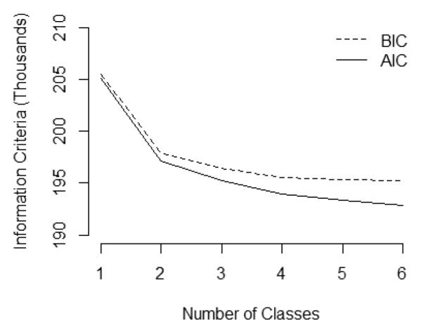
Information criteria as a function of the number of latent classes

Hazard functions for the five class solution, representing the unique risk of event occurrence at a given age or the probability of event occurrence given the event had not yet occurred are displayed in Figure 3. The lifetime distribution functions, displaying the cumulative probability of event occurrence by a given age, are shown in Figure 4. The median event time for an event process within a latent class occurs when the lifetime distribution function is equal to 0.50 (Table 3).

Figure 3.

Hazard functions for five class solution

Figure 4.

Lifetime distribution functions for five class solution

Table 3.

Median event time within latent classes

Class	Label	Work	Marriage	Parent	College
1	WF	<18	22.5	24.5	-
2	CF	21.5	23.5	26.5	21.5
3	CW	21.5	-	-	21.5
4	EP	<18	24.5	18.5	-
5	W	<18	-	-	-

In the five class solution, the first class $({\widehat{\pi }}_1=0.168)$ is characterized by high early risk of work $({\widehat{h}}_{18}=0.63)$, followed by an increasing risk of transition into family roles. The risk of marriage starts low $({\widehat{h}}_{18}=0.03)$ and increases rapidly to a high risk of 0.80 at age 29. The median event time for marriage is in between ages 21 and 22, with nearly a 1.00 cumulative probability of marriage by age 30. The risk of parenthood also starts low $({\widehat{h}}_{18}<0.01)$, and increases in a linear fashion, though the risk is never as high as that for marriage for any specific age (e.g. $({\widehat{h}}_{28}=0.24)$). By age 30, the model implied probability of being a parent is 0.86 for this class, with the median parenthood age between ages 24 and 25. The risk of college graduation is low throughout all of the time periods (maximum is ${\widehat{h}}_{29}=0.03$), with a small cumulative probability of graduating college by age 30 $({\widehat{D}}_{30}=0.17)$. This first class will be labeled a “work then family” pathway (WF).

The second class $({\widehat{\pi }}_2=0.102)$ is characterized by a moderate risk of transitioning into both college and work roles in the mid-twenties, followed by an increasing risk of transitioning into parent and marriage roles in the later twenties. Specifically, the risk of college peaks around ages 22 $({\widehat{h}}_{22}=0.42)$ and the risk of work also peaks around ages 22 to 24 $({\widehat{h}}_{22}=0.43,{\widehat{h}}_{24}=0.45)$. The median age for both beginning full-time work and for college graduation is between ages 21 and 22. The risk of transitioning into marriage is relatively low in the early twenties $({\widehat{h}}_{22}=0.15)$ but increases into the late twenties $({\widehat{h}}_{27}=0.58)$. Risk of parenthood similarly is low in the early twenties $({\widehat{h}}_{22}=0.04)$, but steadily increases throughout the twenties $({\widehat{h}}_{30}=0.41)$. The median age of marriage is between 23 and 24 with nearly a 1.00 probability of marriage by age 30, and the median age of parenthood is between 26 and 27, with high probability of parenthood by age 30 $({\widehat{D}}_{30}=0.88)$. This second class will be labeled a “college then family” pathway (CF).

The third latent class $({\widehat{\pi }}_3=0.217)$ is characterized by moderate risk of college and work in the mid-twenties, similar to the CF pathway mentioned previously, only the risk of transitioning into any family role is low throughout the entire period under study. The risk of college is moderate, at least above 0.20, for all ages after 21. The risk is especially high at age 22 $({\widehat{h}}_{22}=0.42)$ and age 30 $({\widehat{h}}_{30}=0.61)$. The median college graduation age is between 21 and 22, with a 0.99 probability of graduating college by age 30. The risk of work is similarly moderate for all time periods after age 21 (e.g. ${\widehat{h}}_{22}=0.37,{\widehat{h}}_{30}=0.36$), with a 0.98 probability of transitioning into full-time work by age 30. The risk of transitioning into a parent role is less than 0.03 for all ages, and the risk of marriage is similarly low, peaking at 0.11 at age 28. By age 30, there is a 0.38 cumulative probability of transitioning into marriage and only a 0.09 cumulative probability of transitioning into parenthood. This will be labeled a “college and work” pathway (CW).

The hazard functions for the fourth latent class $({\widehat{\pi }}_4=0.222)$ look remarkably different than the other classes, in that the risk for all events decreases over time and the risk of transitioning into a parent role is especially high at early ages. At age 18, the risk of beginning full-time work is 0.59 and the risk of parenthood is 0.35. The median age for beginning full-time work is less than age 18, with a cumulative probability of beginning full-time work of 0.95 by age 30. While decreasing in magnitude, the risk of parenthood remains high in comparison to the other latent classes (e.g. ${\widehat{h}}_{22}=0.30$ compared to ${\widehat{h}}_{22}=0.13$ in the WF pathway). The cumulatively probability of becoming a parent is 0.70 as early as age 20 and reaches 0.90 by age 24. The risk of marriage is also the highest at age 18 $({\widehat{h}}_{18}=0.15)$ and decreases throughout the time period under study $({\widehat{h}}_{30}=0.05)$, with the median marriage time between ages 24 and 25. The risk of college graduation is very low throughout the entire time period (maximum ${\widehat{h}}_{26}=0.02$), with a small cumulative probability of graduating college by age 30 $({\widehat{D}}_{30}=0.13)$. This class will be labeled “early parenthood” pathway (EP).

In the fifth class $({\widehat{\pi }}_5=0.291)$, the risk for transitioning into family roles as well as the risk of college is extremely low throughout all of the time periods, and the risk of work is highest at early ages and then decreases. The risk of work is 0.54 at age 18, and quickly and steadily decreases, with a risk of less than 0.10 of beginning full-time work for each age after 23. The median age for transitioning into full-time work is less than age 18, with a 0.90 cumulative probability by age 30. The risk of marriage is never higher than 0.05 for any age, nor is the risk of parenthood or college graduation. The cumulative probability of transitioning into marriage is 0.23 by age 30, and is 0.26 for parenthood. The cumulative probability of graduating college by age 30 is 0.13. As this class is characterized almost completely by the transition into a work role only, this class will be labeled “work” (W).

Examining results for the six class solution revealed a substantively redundant latent class, resulting in the five class solution being selected as the final solution. In the six class solution, the main difference is that the third class from the five class solution – the “college and work” pathway – split into two separate classes, which were nearly identical. Thus, the increase in complexity from a five to a six class solution was not warranted in that it did not substantially increase our ability to describe heterogeneity in the hazard functions. The five class solution was selected as the optimal number of classes, and covariates were then entered into the model to predict class membership.⁵ By selecting the number of classes without covariates and then comparing the solution to that obtained with covariates predicting class membership, the stability of the model can be investigated. In the model with covariates predicting class membership only, an assumption is made that all effects of covariates on the hazard functions are transmitted through the latent class variable, which should hold as long as the number of latent classes is sufficient to fully capture heterogeneity in the hazard functions. If the size or substantive interpretation of the classes changes, this may indicate that too few classes have been selected and that the assumption that the covariates only influence class membership is violated (Petras & Masyn, 2010; Marsh, Lüdtke, Trautwein, & Morin, 2009).

In this case, the size of the classes as well as the parameter estimates remained stable after the covariates were entered into the model. As another check on the model, if we compare the aggregate model implied lifetime distribution functions and the sample observed lifetime distribution functions, we find that the average difference between the two sets of functions is small, SRD < 0.001. The difference between the aggregate model implied hazard functions and sample observed hazard functions is also small, SRH = 0.001. Thus, the model is capturing the observed overall risk of event occurrence well, as is expected with unstructured hazard functions.

Because the covariates predict class membership, their effects can be interpreted to indicate how the odds of experiencing each pattern of event histories are influenced. A complete list of all possible odds ratios is given in Table 4, with confidence intervals listed below the estimate, computed with a Bonferroni correction for multiple comparisons with α = 0.05. This table reveals that gender, ethnicity, and parental education all significantly influence latent class membership, as several confidence intervals do not include 1 for each group of predictors.

Table 4.

Odds ratios for five class solution

		Gender	Ethnicity			Parental Education
Class	Intercept	Female	Black	Hispanic	Other	No degree	College
WF v. W	0.63 [0.35,1.15]	1.68 [0.71,4.00]	0.15 [0.06,0.41]	0.58 [0.30,1.11]	0.72 [0.34,1.53]	1.05 [0.54,2.06]	1.00 [0.64,1.55]
CF v. W	0.10 [0.04,0.27]	4.74 [2.46,9.15]	0.30 [0.15,0.57]	0.28 [0.11,0.72]	0.74 [0.35,1.55]	0.46 [0.16,1.29]	3.26 [1.60,6.63]
CW v. W	0.25 [0.14,0.44]	2.39 [1.54,3.73]	0.45 [0.24,0.86]	0.54 [0.26,1.13]	1.24 [0.68,2.26]	0.40 [0.15,1.08]	4.00 [2.52,6.33]
EP v. W	0.37 [0.11,1.22]	4.94 [2.95,8.26]	1.31 [0.56,3.08]	1.06 [0.45,2.50]	0.98 [0.44,2.16]	1.01 [0.61,1.67]	0.73 [0.51,1.04]
WF v EP	1.71 [0.59,4.90]	0.34 [0.17,0.67]	0.11 [0.02,0.55]	0.55 [0.22,1.38]	0.74 [0.24,2.25]	1.04 [0.62,1.76]	1.37 [0.89,2.12]
CF v EP	0.28 [0.05,1.59]	0.96 [0.46,2.01]	0.23 [0.09,0.60]	0.27 [0.12,0.60]	0.76 [0.31,1.85]	0.45 [0.18,1.18]	4.49 [2.40,8.42]
CW v EP	0.67 [0.26,1.69]	0.48 [0.32,0.74]	0.34 [0.12,1.03]	0.51 [0.23,1.15]	1.27 [0.52,3.10]	0.40 [0.16,0.99]	5.51 [3.22,9.43]
WF v CW	2.55 [1.48,4.42]	0.70 [0.32,1.57]	0.33 [0.11,1.01]	1.06 [0.52,2.17]	0.58 [0.24,1.40]	2.60 [1.01,6.79]	0.25 [0.15,0.42]
CF v CW	0.41 [0.12,1.46]	1.98 [1.04,3.77]	0.66 [0.33,1.30]	0.52 [0.23,1.17]	0.60 [0.28,1.28]	1.14 [0.28,4.60]	0.81 [0.35,1.88]
WF v CF	6.16 [1.89,20.02]	0.36 [0.11,1.16]	0.51 [0.16,1.57]	2.05 [0.79,5.33]	0.98 [0.36,2.68]	2.29 [0.74,7.04]	0.31 [0.14,0.67]

For brevity purposes, we can generalize over these findings, and we see that females are generally more likely to be in the early parenthood pathway, and males are generally more likely to be in the work pathway. The model implies that African-Americans are generally more likely to be in the work pathway and the early parenthood pathway than Caucasians. Similarly, Hispanics are more likely to be in the work pathway and the early parenthood pathway than the college then family pathway than Caucasians. No differences between those of other ethnicities and Caucasians were found in terms of predicting class membership. Parental education had an extremely consistent effect, in that the odds for individuals who had at least one parent with a college degree of being in a college pathway compared to any other pathway were significantly higher than for individuals who had a parent with a high school degree only.

The influence of covariates may also be examined by comparing aggregate model implied lifetime distribution functions weighting over latent classes conditional on different levels of the covariates in the model, as discussed in the previous section. In this analysis, we focused on the effect of parental education and computed model implied lifetime distribution functions across different levels of parental education, holding gender constant at male and ethnicity constant at Caucasian (Figure 5, left column). The most dramatic difference between these functions is in terms of the cumulative probability of graduating college; individuals with a parent with a college degree have a much higher probability of graduating college by age 30 $({\widehat{D}}_{30}=0.48)$ than individuals with a parent with a high school degree $({\widehat{D}}_{30}=0.26)$ or no parent completing a high school degree $({\widehat{D}}_{30}=0.20)$ as implied by the model. Related, the model predicts individuals who have a parent with a college degree have a smaller probability of beginning full-time work at earlier ages (e.g. ${\widehat{D}}_{18}=0.37$) than individuals who have a parent with a high school degree $({\widehat{D}}_{18}=0.50)$ or no degree $({\widehat{D}}_{18}=0.54)$, but that there are no virtually no differences after age 24. The model implies that individuals who have a parent with a college degree also have a smaller risk of parenthood across all ages, and a smaller risk of marriage at earlier ages, but that the cumulative probability of marriage by age 30 is similar across parental education groups (range for 30 ${\widehat{D}}_{30}=0.54-0.55$).

Figure 5.

Model implied versus sample observed lifetime distribution functions, depending on parental education

Stratifying the Add Health sample by parent education and examining only Caucasian males for comparison purposes resulted in a sample size of 222 for neither parent with a high school degree, 944 for at least one parent with a high school degree only, and 2,536 for at least one parent with a college degree. The trends described by the model implied functions were found in the stratified sample observed functions in that those who had a parent with a college degree were much more likely to graduate college (D₃₀ = 0.50) than for individuals who had neither parent graduate high school or at least one parent graduate high school but who had no further education (D₃₀ = 0.07 and D₃₀ = 0.22, respectively) (Figure 5, right column).

Note, however, that the model underestimated differences between these groups in that it overestimated the probability of graduating college for those with neither parent graduating high school (model implied ${\widehat{D}}_{30}=0.20$; sample estimated D₃₀ = 0.07). The trend was also consistent between the model implied and sample observed functions for work, with individuals with a parent with a college degree having a delay in the transition to full-time work (D₁₈ = 0.39 versus parent with a high school degree D₁₈ = 0.62). Also as implied by the model, individuals with a parent with a college degree had a smaller probability of parenthood across all ages as well as a smaller probability of marriage at early ages. Overall, the average difference between the model implied functions and the sample observed functions across the three parental educations categories was small, SRD = 0.03.

It is unclear whether the differences found between the sample observed lifetime distribution functions and the model implied functions weighting over latent classes are due to utilizing relatively few classes to capture the multivariate distribution of events, or due to possible minor misspecifications in the multinomial model for class membership, such as the omission of interaction effects. However, considering the small number of covariates included in the model, and the relatively simple expression of covariate effects, the model appears to be relatively stable and to be reproducing the observed patterns well.

Discussion

A discrete-time multiple event process survival mixture (MEPSUM) model was introduced in this paper, which allows researchers to investigate the order and timing of multiple non-repeatable events that can occur at the same point in time. Both to be consistent with theory, as well as to understand how the events are related to each other, it is important to consider the relationship between the hazard functions rather than to dissect the events in order to apply more traditional methods. This model is proposed as an indirect application of mixture modeling, as it is employed as a mathematical device – a way to summarize the risk of multiple events. Thus, rather than subjectively classifying individuals based on their response patterns and examining the resulting hazard functions within those groups, the model recognizes uncertainty in group membership and allows the examination of predictors on latent classes (Nagin, 1999).

Importantly, the MEPSUM model is a data-driven method, and the inclusion of auxiliary information is essential to understanding the utility of the latent classes which are derived from the model (Petras & Masyn, 2010). To the extent that the events are related, the model will require multiple latent classes to capture these associations, regardless of whether event times differ qualitatively or quantitatively across individuals. This interpretation of the latent classes is similar to growth mixture models, in which classes may or may not represent qualitatively distinct groups (Bauer & Curran, 2003). The classes obtained from a MEPSUM model provide a glimpse of prototypical multivariate pathways, and thus of how event times are related, but they should not be regarded as representing all possible pathways. Ultimately, examining how the heterogeneity in classes is influenced by covariates should be the end focus of the analysis. As Nagin and Odgers (2010) argue for a related model, the purpose of latent groups in this model is to draw attention to differences in the causes and consequences of different pathways rather than to suggest the population is composed of literally distinct groups.

In the empirical example in this paper, the MEPSUM model was used to capture heterogeneity in the hazard functions for multiple life course events. It provided information on how life events differ in their timing and configuration across people, with five prototypical event history patterns: work then family, college then family, college without family, early parenthood, and work only. It also found that gender, ethnicity, and parental education all significantly influenced the occurrence and relative timing of life transitions in adolescence and young adulthood. The large sample size allowed stratification of the sample by different levels of covariates and comparison of model implied functions to sample estimated functions. Overall, there was general consistency in the functions implied by the model and the sample observed functions, such as females having a larger probability of parenthood at earlier ages than males. It should be noted that a relatively large sample size may be required for this model, as it aims to model heterogeneity in multiple hazard functions (guidelines on what exactly constitutes a “large sample size” will require extensive simulation studies and should be the subject of future research).

A limitation of this work is that only a small number of covariates were examined in the empirical example, both for simplicity purposes as well as so sample stratified functions could be calculated to investigate model performance. How the model performs with numerous covariates and with more complicated inclusions of covariates is yet to be seen. Potentially interesting directions for future research would be to investigate model performance with additional covariates, and consideration of how the addition of direct effects of covariates on the hazard functions could impact the performance of the model. A “multiple groups” version of the model could also be of interest, in which separate latent classes are estimated within each of two or more predefined subpopulations (e.g., males and females) and invariance tests are implemented to evaluate whether the pathways obtained across these subpopulations are similar or dissimilar.

An additional issue in need of further consideration is the adequacy of the approximation provided by the finite mixture form for the underlying multivariate hazard distribution. Research conducted on a related model, the semi-parametric groups-based trajectory model (SPGM; see Nagin, 1999), is pertinent to this question. Like the MEPSUM, the SPGM uses a discrete-point finite mixture to approximate an underlying distribution, namely the distribution of random effects underlying individual differences in change over time. Simulation research on the SPGM conducted by Brame et al. (2006), Nagin (2005), and Muthén and Asparouhov (2008) has demonstrated that a discrete-point finite mixture can reasonably approximate various random effects distributions of low dimensionality. More recently, however, Sterba, Baldasaro and Bauer (2012) determined that the adequacy of the approximation suffers when the random effects distribution is of higher dimensionality, particularly for binary outcomes at low sample sizes. The latter results give greater emphasis to our caution that the MEPSUM model is likely to perform best in large samples. Although these results are informative, it is also worth noting a key difference between the SPGM and MEPSUM. Whereas there are widely used alternative models to SPGM for capturing individual differences in growth trajectories (e.g., multilevel growth models or latent curve models), to our knowledge no alternative models currently exist for modeling a multivariate distribution of hazard functions. Further research developing and comparing alternative approaches for modeling multiple event processes should thus be encouraged.

While there are many possible directions for future research, it is our hope that the model proposed in this paper will provide a useful framework from which to evaluate the interdependencies of multiple event processes measured in discrete time.

References

- Abar B, Loken E. Consequences of fitting nonidentified latent class models. Structural Equation Modeling: A Multidisciplinary Journal. 2012;19:1–15. [Google Scholar]
- Akaike H. A new look at statistical model identification. IEEE Transactions on automatic Control, AU. 1974;19:719–722. [Google Scholar]
- Allison PD. Logistic regression using the SAS system: Theory and application. SAS Institute; Cary, N.C: 1999. [Google Scholar]
- Bandeen-Roche K, Miglioretti DL, Zeger SL, Rathouz PJ. Latent variable regression for multiple discrete outcomes. Journal of the American Statistical Association. 1997;92:1375–1386. [Google Scholar]
- Bauer DJ, Curran PJ. Distributional assumptions of growth mixture models: Implications for overextraction of latent trajectory classes. Psychological Methods. 2003;8:338–363. doi: 10.1037/1082-989X.8.3.338. [DOI] [PubMed] [Google Scholar]
- Bowers AJ. Grades and Graduation: A Longitudinal Risk Perspective to Identify Student Dropouts. Journal of Educational Research. 2010;103(3):191–207. [Google Scholar]
- Bozdogan H. Model selection and Akaike’s Information Criterion (AIC): The general theory and its analytical extensions. Psychometrika. 1987;52:345–370. [Google Scholar]
- Brame R, Nagin DS, Wasserman L. Exploring some analytical characteristics of finite mixture models. Journal of Quantitative Criminology. 2006;22:31–59. [Google Scholar]
- Bray BC, Lanza ST, Collins LM. Modeling Relations among Discrete Developmental Processes: A General Approach to Associative Latent Transition Analysis. Structural Equation Modeling. 2010;17(4):541–569. doi: 10.1080/10705511.2010.510043. [DOI] [PMC free article] [PubMed] [Google Scholar]
- Celeux G, Biernacki C, Govaert G. Technical report. INRIA; Rhone-Alpes: 1997. Choosing models in model-based clustering and discriminant analysis. [Google Scholar]
- Collins LM, Lanza ST. Latent class and latent transition analysis. John Wiley & Sons, Inc.; Hoboken, New Jersey: 2010. [Google Scholar]
- Corning AF, Malofeeva EV. The application of survival analysis to the study of psychotherapy termination. Journal of Counseling Psychology. 2004;51(3):354–367. [Google Scholar]
- Elder GH., Jr. Life Course Dynamics. Cornell University Press; Ithaca, NY: 1985. [Google Scholar]
- Fraley C, Raftery AE. Technical report No. 329. Department of Statistics, University of Washington; 1998. How many clusters? Which clustering method? Answers via model-based cluster analysis. [Google Scholar]
- Gabadinho A, Ritschard G, Müller NS, Studer M. Analyzing and visualizing state sequences in R with TraMineR. Journal of Statistical Software. 2011;40(4):1–37. [Google Scholar]
- Ha JC, Kimpo CL, Sackett GP. Multiple-spell, discrete-time survival analysis of developmental data: Object concept in pigtailed macaques. Developmental Psychology. 1997;33(6):1054–1059. doi: 10.1037//0012-1649.33.6.1054. [DOI] [PubMed] [Google Scholar]
- Harris KM, Halpern CT, Whitsel E, Hussey J, Tabor J, Entzel P, Udry JR. The National Longitudinal Study of Adolescent Health: Research Design. 2009 http://www.cpc.unc.edu/projects/addhealth/design.
- Heckman J, Singer B. A method for minimizing the impact of distributional assumptions in econometric models for duration data. Econometrica. 1984;52:271–320. [Google Scholar]
- Hipp JR, Bauer DJ. Local solutions in the estimation of growth mixture models. Psychological Methods. 2006;11(1):36–53. doi: 10.1037/1082-989X.11.1.36. [DOI] [PubMed] [Google Scholar]
- Hougaard P. Analysis of multivariate survival data. Springer; New York: 2000. [Google Scholar]
- Kish L. Survey Sampling. John Wiley & Sons; New York: 1965. [Google Scholar]
- Lee ET, Wang JW. Statistical Methods for Survival Data Analysis. J. Wiley; New York: 2003. [Google Scholar]
- Lo Y, Mendell NR, Rubin DB. Testing the number of components in a normal mixture. Biometrika. 2001;88(3):767–778. [Google Scholar]
- Lohr S. Sampling: Design and Analysis. Duxbury Press; Pacific Grove: 2009. [Google Scholar]
- Macmillan R, Eliason SR. Characterizing the life course as role configurations and pathways: A latent structure approach. In: Mortimer JT, Shanahan MJ, editors. Handbook of the life course. Kluwer Academic Publishers; Hingham, MA: 2003. [Google Scholar]
- Mahaffy KA. Gender, race, class, and the transition to adulthood: A critical review of the literature. Sociological Studies of Children and Youth. 2003;9:15–47. [Google Scholar]
- Malone PS, Lamis DA, Masyn KE, Northrup TF. A dual-process discrete-time survival analysis model: Application to the gateway drug hypothesis. Multivariate Behavioral Research. 2010;45(5):790–805. doi: 10.1080/00273171.2010.519277. [DOI] [PMC free article] [PubMed] [Google Scholar]
- Mare RD. Discrete-time bivariate hazards with unobserved heterogeneity: A partially observed contingency table approach. In: Marsden PV, editor. Sociological Methodology 1994. Basil Blackwlel; Oxford: 1994. pp. 341–85. [Google Scholar]
- Marini M. Women’s educational attainment and the timing of entry into parenthood. American Sociological Review. 1984;49(4):491–511. [Google Scholar]
- Marsh HW, Lüdtke O, Trautwein U, Morin A. Classical latent profile analysis of academic self-concept dimensions: Synergy of person- and variable-centered approaches to theoretical models of self-concept. Structural Equation Modeling: A Multidisciplinary Journal. 2009;16:191–225. [Google Scholar]
- McLachlan G, Peel D. Finite Mixture Models. Wiley; New York: 2000. [Google Scholar]
- Muthén B, Asparouhov T. Growth mixture modeling: Analysis with non-Gaussian random effects. In: Davidian FG, Verbeke MG, Mohlenberghs G, editors. Longitudinal data analysis. Chapman & Hall / CRC Press; Boca Raton, FL: 2008. pp. 143–165. [Google Scholar]
- Muthén B, Masyn K. Discrete-Time Survival Mixture Analysis. Journal of Educational and Behavioral Statistics. 2005;30(1):27–58. [Google Scholar]
- Muthén LK, Muthén BO. Mplus User’s Guide. Sixth Edition Muthén & Muthén; Los Angeles, CA: 1998-2010. [Google Scholar]
- Nagin DS. Analyzing developmental trajectories: A semiparametric group-based approach. Psychological Methods. 1999;2:139–157. doi: 10.1037/1082-989x.6.1.18. [DOI] [PubMed] [Google Scholar]
- Nagin DS. Group-based modeling of development. Harvard University Press; Cambridge, MA: 2005. [Google Scholar]
- Nagin DS, Land KC. Age, criminal careers, and population heterogeneity: specification and estimation of a nonparametric mixed Poisson model. Criminology. 1993;31:327–362. [Google Scholar]
- Nagin DS, Odgers CL. Group-based trajectory modeling in clinical research. Annual Review of Clinical Psychology. 2010;6:109–138. doi: 10.1146/annurev.clinpsy.121208.131413. [DOI] [PubMed] [Google Scholar]
- Nylund KL, Asparouhov T, Muthén BO. Deciding on the number of classes in latent class analysis and growth mixture modeling: A Monte Carlo simulation study. Structural Equation Modeling: A Multidisciplinary Journal. 2007;14(4):535–569. [Google Scholar]
- Petras H, Masyn K. General growth mixture analysis with antecedents and consequences of change. In: Piquero A, Weisburd D, editors. Handbook of Quantitative Criminology. Springer; New York: 2010. pp. 69–100. [Google Scholar]
- Schwartz SJ, Phelps E, Lerner JV, Shi H, Brown C, Lewin-Bizan S, Li Y, Lerner RM. Promotion as prevention: Positive youth development as protective against tobacco, alcohol, illicit drug, and sex initiation. Applied Developmental Science. 2010;14(4):197–211. [Google Scholar]
- Schwarz G. Estimating the dimensions of a model. Annals of Statistics. 1978;6:461–464. [Google Scholar]
- Scott KM, Wells JE, Angermeyer MM, Brugha TS, Bromet EE, Demyttenaere KK, Kessler RC. Gender and the relationship between marital status and first onset of mood, anxiety and substance use disorders. Psychological Medicine: A Journal of Research in Psychiatry and the Allied Sciences. 2010;40(9):1495–1505. doi: 10.1017/S0033291709991942. [DOI] [PMC free article] [PubMed] [Google Scholar]
- Shanahan M. Pathways to adulthood in changing societies: Variability and mechanisms in life course perspective. Annual Review of Sociology. 2000;26:667–692. [Google Scholar]
- Shanahan M, Miech R, Elder G. Changing pathways to attainment in men’s lives, historical patterns of school, work, and social class. Social Forces. 1998;77:231–256. [Google Scholar]
- Singer JD, Willett JB. Applied longitudinal data analysis: Modeling change and event occurrence. Oxford University Press; New York: 2003. [Google Scholar]
- Sterba SK, Baldasaro RE, Bauer DJ. Factors affecting the adequacy and preferability of semiparametric groups-based approximations of continuous growth trajectories. Multivariate Behavioral Research. 2012;47:590–634. doi: 10.1080/00273171.2012.692639. [DOI] [PubMed] [Google Scholar]
- Vermunt JK. Log-linear models for event histories. Sage; Thousand Oaks, CA: 1997. [Google Scholar]
- Vermunt JK, Magidson J. Latent class cluster analysis. In: Hagenaars J, McCutcheon A, editors. Applied latent class analysis. Cambridge University Press; Cambridge, UK: 2002. pp. 89–106. [Google Scholar]
- Vermunt JK, Magidson J. Latent GOLD 4.0 Choice User’s Guide. Statistical Innovations Inc.; Belmont Massachussetts: 2005. [Google Scholar]