Quantifying ChIP-seq data: a spiking method providing an internal reference for sample-to-sample normalization

Abstract

Chromatin immunoprecipitation followed by deep sequencing (ChIP-seq) experiments are widely used to determine, within entire genomes, the occupancy sites of any protein of interest, including, for example, transcription factors, RNA polymerases, or histones with or without various modifications. In addition to allowing the determination of occupancy sites within one cell type and under one condition, this method allows, in principle, the establishment and comparison of occupancy maps in various cell types, tissues, and conditions. Such comparisons require, however, that samples be normalized. Widely used normalization methods that include a quantile normalization step perform well when factor occupancy varies at a subset of sites, but may miss uniform genome-wide increases or decreases in site occupancy. We describe a spike adjustment procedure (SAP) that, unlike commonly used normalization methods intervening at the analysis stage, entails an experimental step prior to immunoprecipitation. A constant, low amount from a single batch of chromatin of a foreign genome is added to the experimental chromatin. This “spike” chromatin then serves as an internal control to which the experimental signals can be adjusted. We show that the method improves similarity between replicates and reveals biological differences including global and largely uniform changes.

In chromatin immunoprecipitation (ChIP) followed by deep sequencing (ChIP-seq) (Barski et al. 2007; Johnson et al. 2007a; Mikkelsen et al. 2007), chromatin is first treated, within intact cells, with a cross-linking reagent such as formaldehyde. The cross-linked chromatin is then isolated and fragmented, often by sonication, and used as starting material for immunoprecipitations with antibodies directed against the factors of interest. The immunoprecipitated material, containing the protein targeted by the antibody as well as any DNA cross-linked to it, is heated to reverse the crosslinks, the DNA is purified, and an amplified representation of this DNA is submitted to deep sequencing. Deep sequencing generates sequence “tags” of commonly 35 to ∼100 nucleotides (nt), which are then aligned onto the genome. Genomic regions enriched in aligned tags over noise (variously defined in different works) are interpreted as regions of factor occupancy. This method has proven immensely powerful in characterizing chromatin organization, i.e., in identifying sites bound, for example, by transcription factors, by histones carrying (or not) specific modifications, or by RNA polymerases.

Apart from identifying regions of factor occupancy within a single chromatin sample, ChIP-seq is invaluable for comparing the level of occupancy at a set of loci (e.g., previously identified targets of a specific transcription factor) between different chromatin samples from various cell types or tissues, from cells submitted to different conditions, or from cells at different developmental stages, etc. Unlike measurements of mature mRNAs, such experiments inform on changes occurring at the very first steps of gene expression, i.e., changes in chromatin structure and gene transcription. In such experiments, however, reliable sample normalization has proven difficult.

There are a number of different methods to normalize ChIP-seq samples including scaling to total amounts of tags (i.e., normalizing for sequencing depth), quantile normalization, and other methods. Scaling to the total amount of sequence tags that can be aligned onto the genome is usually the first step (for examples, see Li et al. 2011; Landt et al. 2012; Le Martelot et al. 2012). Quantile normalization is also broadly applied because it can reveal differences at specific loci even in samples displaying relatively uniform global differences at all enriched loci (for examples, see Rahl et al. 2010; Le Martelot et al. 2012). Scaling to total tag amounts and quantile normalization can have very different effects, particularly in cases of global differences; for example, if all regions enriched in one sample are uniformly enriched to a higher or lower degree in another sample. With just scaling to total amount of aligned tags, these differences might persist, but their interpretation will be difficult because scaling will not distinguish whether the differences result from technical experimental variations or from genuine biological differences. With quantile normalization, on the other hand, the distributions of the various samples are made identical so that they can be easily compared, thus masking any uniform changes, whether genuine or not, from one sample to another.

Here we describe a spike adjustment procedure (SAP) designed to allow comparison of occupancy levels for a set of loci of interest. Unlike the above, this method addresses the problem via an experimental procedure conducted prior to immunoprecipitation. It consists of adding a constant, low amount of a single batch of foreign chromatin (e.g., human) as an internal control to each sample of the chromatin of interest (e.g., mouse) before immunoprecipitation. This allows adjustment of the signals in each sample to the internal control. We show that unlike only scaling to the total amount of aligned sequence tags or quantile normalization, the SAP allows the scoring of global and largely uniform changes when they result from biological differences.

Results

To illustrate the approach, Figure 1A shows a hypothetical experiment in which all ChIP-seq peaks are higher in a first sample (light blue) compared with a second sample (purple). The global change in peak size could in principle be the result of a biological difference, e.g., occupancy in the second example might be reduced because of some change in cell metabolism; or it might reflect a technical problem such as reduced immunoprecipitation efficiency. In this hypothetical example, scaling to total amount of tags maintains the differences because the total number of sequenced and aligned tags is roughly similar in both samples (Fig. 1B). In contrast, scaling followed by quantile normalization reveals almost no differences between the samples (Fig. 1C), because the peaks in the second experiment are more or less uniformly lower than in the first. Thus, in this example the two methods give different results and do not allow one to distinguish between the two scenarios, genuine biological difference or technical variability. The two scenarios should be distinguishable, however, by adjustment to an internal reference. In panels D and E, the same experiment is shown as in panel A but this time with a spike signal, symbolized by the yellow bars. Replicates (or similar biological samples) displaying apparent different occupancy due to technical problems would display a lower spike signal in the second sample and, after normalization to this internal reference by the SAP, little or no change (Fig. 1F). In contrast, biologically different samples would reveal a global negative fold change (Fig. 1G).

Figure 1.

Normalization can obscure global effects. (A) Schematic representation of peaks obtained after ChIP-seq in a hypothetical example where all peaks are uniformly diminished in the second (purple) sample compared with the first (light blue). These samples can represent a replicate experiment, in which case the overall decrease observed in the second sample is the result of experimental variation, or they can represent experiments performed with samples collected under different conditions, in which case the global decrease might reflect a biological difference. No spike chromatin is included. (B) Normalization by scaling to total number of tags aligned onto the genome (i.e., normalization for sequencing depth) showing tag counts (top) and log₂ fold change (bottom). In this hypothetical example, the number of tags aligned onto the genome is quite similar in both samples, and this type of normalization indicates a general decrease for each peak in the second sample, whether the two samples are biologically different (and thus should indeed indicate a protein occupancy decrease in sample 2) or similar (and thus should in fact display similar signals). (C) Normalization by scaling followed by quantile normalization showing tag counts (top) and log₂ fold change (bottom). In this example, the second step—quantile normalization—will equalize the sample distributions whether the samples are biologically different or not, because the decrease in sample 2 is uniform. In D and E, spike chromatin is included in the sample and gives rise to signals symbolized by the yellow bars. (F,G) Normalization by scaling followed by spike adjustment showing tag counts (top) and log₂ fold change (bottom). In F, the spike adjustment factor increased the signals in sample 2 by a factor of about two, in G, the spike adjustment factor decreased the signal in sample 2 by a factor of about 0.8 (see yellow bars). Spike adjustment reveals whether the samples are in fact similar (example in F) or are in fact biologically different (example in G).

Addition of different percentages of human chromatin to mouse chromatin

An internal reference is most useful when included as early as possible in an experimental procedure. We therefore sought to include the internal reference before the immunoprecipitation step, which is one of the steps likely to generate variation from one sample to another in the ChIP-seq protocol. We tested the usefulness of adding spikes of human chromatin to mouse chromatin samples for ChIP-seq experiments performed with two antibodies: one directed against POLR3D (RPC4), a subunit of RNA polymerase (Pol) III; and the other against POLR2B (RPB2), the second largest subunit of Pol II (for a list of the samples used in this work and their nomenclature, see Table 1). Both antibodies are directed against peptides that are 100% conserved in mouse and human Pol III and Pol II, respectively. We first focused on experiments using the anti-POLR3D antibody and tested mixing different amounts of human chromatin with the mouse chromatin, with the aim of using the smallest possible amount of human chromatin so as to avoid unnecessary contamination of the mouse sample, and yet obtaining a robust signal on a sufficient number of human genes.

Table 1.

Samples used in this work

The various mixtures were used for ChIP-seq and the resulting 100-nt-long sequence tags were aligned with both the mouse (NCBI37/mm9) and human (GRCh37/hg19) genomes. Supplemental Table S1, A and B, lists the tag counts that aligned to the mouse genome, the human genome, or to both genomes (ambiguous tags). Adding 2.5%, 5%, or 10% human chromatin derived from HeLa cells resulted in an increase in the number of reads aligning to the human genome, as expected, but had little influence on the amount of ambiguous reads, indicating that most of the ambiguous reads originate from the mouse chromatin, which is not surprising since this chromatin represents in all cases most of the material. Moreover, the ambiguous tags represented only a small proportion of the tags mapping to human Pol III regions (see Supplemental Table S1B [sheet 2], last column) such that there was little loss of sensitivity in the human signal due to the exclusion of tags that cannot be unequivocally mapped to the mouse or human genomes. For subsequent analyses, we thus used 2.5% human chromatin, as this amount produced a usable signal on human genes (see below).

Spiking samples allows quality control

Figure 2 summarizes the steps in the SAP. After tag alignment to the human and the mouse genomes and removal of ambiguous tags, we first tested whether the human spike signal can be used for quality control evaluation. Indeed, since the human chromatin added to the experimental mouse samples is constant from one sample to another, the quality of the human signal should in principle attest to the technical quality of the experiment, unlike experimental mouse samples where the mouse signal may vary according to biological differences. We thus compared a sample generated with our standard protocol (90_R1) (see Table 1) to a “poor” sample (97.5_P1) (see Table 1) in which we deliberately contaminated the immunoprecipitated material by adding back 1.5% of the supernatant obtained after immunoprecipitation. Figure 3 shows, for each of these two spiked-in samples, a mean-difference scatter plot comparing spike human tag counts in 400-bp genomic bins obtained in the ChIP versus the input. The red dots indicate bins that overlap with what we refer to hereafter as “Pol III loci,” i.e., annotated Pol III genes (whether occupied by Pol III or not) as well as previously identified Pol III–occupied loci (see Table S2 in Renaud et al. 2014). With the standard protocol (upper panel), many of the bins overlapping with spike human Pol III loci showed strong enrichment in the ChIP sample with respect to the input. In contrast, the poor sample (lower panel) showed almost no enrichment. Thus, the amount of signal in human Pol III loci reflects sample quality, as expected, and can be used for quality control. A quantitative metric to characterize signal content can be the percentage of tags aligning in gene regions. Indeed, as shown in Supplemental Table S1B (sheet 2), the percentage of human tags in human Pol III loci was 8.7- to 16.7-fold lower for the poor 97.5_P1 sample compared with the standard 97.5_R1 or any of the other standard replicate (R) samples (column G). Together with visual inspection of scatter plots as shown above, this information can be used to identify samples that should be discarded (and experiments that should be redone).

Figure 2.

Schematic diagram summarizing the SAP. The main steps, i.e., examination of sample quality, scaling to total amount of genome-aligned tags, selection of signal genes, score calculation, and spike adjustment, are numbered.

Figure 3.

The spike chromatin can be used for quality control. Mean-difference scatter plot of human Pol III genome bin counts (in log scale). Red dots indicate genomic bins that overlap with Pol III loci. The genome was binned into 400-bp bins (corresponding to a typical Pol III gene length [∼100 bp] extended by 150 bp in both the upstream and downstream directions). Zero-count bins were filtered out prior to plotting. (A) An example of a good-quality sample (90_R1). (B) An example of a poor-quality sample (97.5_P1).

The next step after assessing sample quality consisted in scaling the samples relative to the total number of aligned tags (scaling for sequencing depth) in each experiment, which was performed separately for the mouse and human tags (Fig. 2, step 2). We then selected signal loci (step 3; see Methods) and calculated scores for the human sample and preliminary scores for the mouse sample (step 4). We then used the sample-to-sample differences in human signals to compute a spike adjustment factor for each sample. This spike adjustment factor was applied to the preliminary scores of the mouse Pol III loci (for a list of these loci, see Table S3 in Renaud et al. 2014) to obtain final scores (step 5; see Methods).

Effect of sonication on the spike signal

As sonication is performed before addition of the spiking material, a possible problem with the SAP might arise as a result of sonication of the human and mouse samples to different average fragment sizes. This is illustrated in Figure 4A. In this example, the human chromatin, which is from a single batch, is sonicated to an average size of 500 bp. In contrast, the first mouse chromatin is sonicated to a larger average size (upper panel), whereas the second sample is sonicated to a smaller average size (lower panel). Size selection of DNA fragments from 200 to 400 bp during library preparation (indicated by the rectangle) would result in a smaller percentage of mouse chromatin in the first case compared with the second case. This problem should be in large part circumvented by the first normalization step, in which we scale independently the human and mouse signals to the total number of aligned sequence tags.

Figure 4.

The SAP tolerates sample-to-sample differences of average chromatin fragment length. (A) Illustration of two hypothetical cases. (Top) The mouse chromatin sample (blue) is sonicated to an average size >500 bp; (bottom) the average size is <500 bp. The human chromatin (red) used to spike the samples is from the same batch and has an average size of 500 bp. Size selection from 200 to 400 bp is expected to result in a smaller proportion of mouse chromatin in the first case than in the second case. (B) Size representation obtained by fragment analyzer (top) and 1% agarose gel electrophoresis (bottom) of three mouse chromatin samples sonicated for 5 (S5), 10 (S10), and 15 (S15) cycles of 10 sec, as indicated above the lanes. The position of DNA size markers (in bp) is indicated on the left. The last lane shows the human chromatin spike sample. (C) Scatter plots showing the relation of mouse Pol III loci scores before and after spike adjustment for the three pairs of samples sonicated for different amounts of time. The Pearson and Spearman correlations before and after spike adjustment were as follows: 97.5_S5 versus 97.5_S10, 0.9927→0.9935 and 0.9678→0.9653; 97.5_S5 versus 97.5_S15, 0.9900→0.9885 and 0.9728→0.9663; and 97.5_S10 versus 97.5_S15, 0.9917→0.9926 and 0.9626→0.9636.

To directly test the effects of different average sizes of the mouse sample, we sonicated mouse chromatin for five, 10, and 15 cycles. As expected, increasing the number of sonication cycles resulted in shorter average mouse chromatin fragment lengths, as visualized after analysis on a Bioanalyzer 2100 from Agilent (Fig. 4B, upper panel, lanes S5, S10, S15) or after agarose gel electrophoresis (lower panel). Figure 4B also shows the human spike chromatin, which was fragmented less completely than the mouse samples but nevertheless contained an abundance of fragments <1000 bp.

Despite the variable length distributions of the mouse chromatin samples, the SAP did not disrupt the data and sample alignments remained very high in all cases, as illustrated by the scatter plots in Figure 4C (for Pearson and Spearman correlations, see Figure 4 legend). Thus, spike adjustment is quite impervious to differences in sample sonication.

Spike adjustment both improves similarity between biological replicates and reveals biological differences

To test the usefulness of the SAP to both improve similarity between replicates and reveal biological differences, we made use of two experiments that are part of an independent study (N Bonhoure, V Praz, RD Moir, IM Willis, and N Hernandez, unpubl.). In these experiments, which were performed at different times, before and after upgrade of the sequencer, but with the same batches of mouse and human chromatin, we compared Pol III occupancy in the liver of wild-type (WT) mice (samples mR1_WT and mR2_WT) (see Table 1) and mice lacking the Maf1 gene (mR1_KO and mR2_KO). MAF1 is a repressor of Pol III transcription, both in yeast (Pluta et al. 2001; Upadhya et al. 2002) and in mammalian cells (Reina et al. 2006; Johnson et al. 2007b; Rollins et al. 2007), which prevents transcription complex assembly by binding to Pol III as well as to BRF1, a member of the Pol III preinitiation complex (Desai et al. 2005; Oficjalska-Pham et al. 2006; Reina et al. 2006; Goodfellow and White 2007; Vannini et al. 2010). In the absence of MAF1, one might expect a difference in Pol III occupancy at Pol III loci.

We first compared the replicates before and after spike adjustment (step 5 in Fig. 2). As shown in the scatter plots in Figure 5, A and B, the scores for Pol III–occupied loci were closer to the x = y line after (black) than before (orange) spike adjustment, both for the replicate samples from WT mice (panel A) and for those of the Maf1 KO mice (panel B).

Figure 5.

Spike adjustment improves similarity between replicates and reveals genuine differences in Pol III occupation. (A,B) Scatter plots showing the relation of Pol III loci scores between the two WT (A) and the two Maf1 KO (B) replicate samples before (orange) and after (black) spike adjustment. The red line corresponds to x = y. (C–E) Boxplot representations of the Pol III loci score distributions for the two WT samples (light and dark green, mR1_WT and mR2_WT) and the two Maf1 KO samples (light and dark blue, mR1_KO and mR2_KO). The scores were normalized to total number of tags aligned onto the genome (C) followed by either quantile normalization (D) or spike adjustment (E). (F–H) Empirical cumulative frequency distributions functions (ECDFs) of the log scores of the indicated distribution. Samples were normalized to the total number of tags aligned onto the genome (F) followed by either quantile normalization (G) or spike adjustment (H). The Kolmogorov-Smirnov (KS) distance for the two WT (green lines) and the two Maf1 KO (blue lines) samples is shown at the bottom right of each panel. (I,J) Mean difference scatter plots illustrating Pol III occupancy in WT and Maf1 KO livers. Samples were normalized to the total number of tags aligned onto the genome followed by quantile normalization (I), respectively by spike adjustment (J). Scores for WT and KO conditions are the average of the two replicates. Loci with scores showing a significant difference in the WT versus Maf1 KO samples are represented with yellow (P ≤ 0.01) and red (0.01 < P ≤ 0.05) dots.

We then compared the four samples using scaling to total number of tags (Fig. 1, cf. A and B), scaling and quantile normalization (Fig. 1, cf. A and C), or scaling and spike adjustment (Fig. 1, cf. D–G). Figure 5, C through E, shows the resulting boxplots of the occupancy scores on Pol III loci in WT (green) and Maf1 KO mice (blue), in the first (light colors) or second (dark colors) experiments. After just scaling (panel C), the average and median occupancy were in each case higher in the Maf1 KO samples compared with the corresponding WT sample. However, the average and mean of the first Maf1 KO sample (mR1_KO) were very similar to the average and mean of the second WT sample (mR2_WT; cf. the second and third box plots), making the results difficult to interpret. Upon scaling and quantile normalization, the distributions of all samples became similar, as expected (panel D). In contrast, the SAP not only remarkably improved the agreement between replicates, in particular for the KO samples, but also revealed a clear difference between the WT and KO samples, with higher average Pol III occupancy in the KO samples (panel E). This was also evident in the empirical cumulative distribution function (ECDF) graphs (panels F–H), showing identical distributions for all samples after scaling and quantile normalization (panel G), but more similar distributions for the two WT and the two KO samples, as well as better separation of the WT and KO sample pairs, for the samples normalized with SAP (cf. panels F and H).

To examine the effect of scaling and quantile normalization versus the SAP on a locus per locus basis, we performed a differential analysis with the two sets of normalized scores. The results are displayed as mean-difference plots in Figure 5, I and J, with the scores showing a significant difference in the WT versus Maf1 KO samples in yellow (P ≤ 0.01) and red (0.01 < P ≤ 0.05). With the scaling and quantile normalization method (panel I), 34 loci had significantly different occupancy, but the minimum false-discovery rate (FDR = 0.045) was close to the cutoff 0.05, and there was a roughly equal number of loci with higher and lower scores in the Maf1 KO compared with the WT samples. With the SAP, 490 loci scored as having significantly different Pol III occupancy, and all but one (with a very low score) showed higher Pol III occupancy in the KO compared with the WT samples (panel J). Thus, the SAP both improves similarity of replicates and reveals biological differences, even when these are quite uniform for all loci.

Improvement of Pol II ChIP-seq biological replicate similarity by spike adjustment

In the examples above, we used a method to calculate preliminary scores (Fig. 2, step 4) that is tailored to ChIP-seq experiments where the total genomic target of the factor of interest is relatively small and where, therefore, the tags mapping to this target represent a small percentage of the total amount of tags aligning onto the genome, as is the case for many factors (Landt et al. 2012). Indeed, for Pol III occupancy, tags mapping to known targets for both human and mouse Pol III (Canella et al. 2010, 2012; Renaud et al. 2014) represented 0.01%–1% of the total number of aligned tags (see Supplemental Table S1A,B). To determine whether the spike adjustment method might be more generally applicable, we applied it to chromatin samples immunoprecipitated with anti-POLR2B antibodies, and we calculated preliminary scores around TSSs using the SPP software (https://sites.google.com/a/brown.edu/bioinformatics-in-biomed/spp-r-from-chip-seq) (Kharchenko et al. 2008). The samples, referred to as RPB2_95 and RPB2_90 (see Table 1), contained different percentages of human chromatin (which was managed in the analysis by the species-specific scaling) (step 2 in Fig. 2) but otherwise were derived from the same batch of mouse chromatin and processed similarly (for numbers of tags aligned to mouse and human genomes, see Supplemental Table S2A,B) and can thus be considered technical replicates. We calculated Pol II scores in mouse regions extending from −250 to +250 bp around 11,217 annotated TSSs selected to be separated by at least 1000 bp from any other annotated TSS or polyadenylation site (see Le Martelot et al. 2012).

Figure 6A, left and right panels, show ECDF graphs of the samples after SPP score calculation, or after SPP score calculation and spike adjustment. The replicates were of high quality such that they were very close even before spike adjustment. Nevertheless, spike adjustment decreased the Kolmogorov-Smirnov distance between the two samples by more than half. The improvement is also visible in the scatter plot in Figure 6B, showing a tightening of the scores along the x = y line after spike adjustment. Thus, spike adjustment performs well not only for samples immunoprecipitated with an antibody targeting Pol III, but also for samples immunoprecipitated with an antibody targeting Pol II. Moreover, it can be applied to scores calculated by a method other than the one we specifically developed for Pol III occupancy. As further discussed below, this method is thus likely to be widely applicable.

Figure 6.

Spike adjustment improves the similarity of two Pol II ChIP-seq replicate experiments. (A) ECDFs of the scores of the indicated distributions. Preliminary scores were computed around the TSS (±250 bp) with the SPP software. The KS distance is shown at the bottom right of each panel. (Dark line) RPB2_90 sample; (light line) RPB2_95 sample. (B) Scatter plots showing the relation between the RPB2_90 and RPB2_95 scores before (orange dots) and after (black dots) spike adjustment. The red line corresponds to x = y.

Discussion

We describe a normalization method for ChIP-seq experiments that is not confined to computational treatment of the data but includes an experimental step, namely the addition of an internal reference to each sample. This internal reference consists of a small amount of chromatin (spike) from a different species than the chromatin being tested, but a species close enough that the factors of interest share conserved epitopes, in our case human chromatin added to mouse chromatin. The internal reference is mixed with the experimental sample and undergoes all experimental steps following fragmentation of the chromatin, i.e., immunoprecipitation, library preparation, and sequencing. The method is related, in its principle of introducing an internal reference into each sample, to the method recently described by Loven et al. (2012) to normalize RNA-seq data. In that case, a synthetic RNA standard is added to each RNA sample to be analyzed in proportion to the starting number of cells, thus allowing quantification of RNA relative to starting cell number (Loven et al. 2012).

We show that the spike signal allows quality control. Indeed, it is in principle affected only by experimental (rather than biological) variations, and thus allows one to pinpoint dubious experimental samples that should be considered with circumspection and possibly discarded. For samples passing this quality control test, the SAP both improves similarity between replicates, without disrupting the distribution of the data, and reliably reveals true biological differences. Thus, on one hand, spike adjustment prevents the erroneous perception of differences when there are no genuine differences in protein occupancy; i.e., it reduces false-positive calls. On the other hand, it allows reliable recognition of real differences in occupancy; i.e., it also reduces false-negative calls.

The amount of spike material to be added to the sample should be as low as possible to give a robust spike signal and yet to contribute as few ambiguous tags as possible. This amount will vary with sequencing depth and size of the ChIP genomic target (for an exploration of this relationship, see Methods). We tested adding different amounts of human “spike” chromatin to the mouse chromatin and found that for our experiments, 2.5% was sufficient to provide a robust spike signal (Fig. 3). It might be advantageous to use as much as 5% spike chromatin because this may allow the “rescue” of poorer quality experimental samples. On the other hand, an increase in spike material might result in an increase in the number of ambiguous tags, i.e., tags that map to both the mouse and the human genomes, and this in turn might affect the mouse scores, especially for lowly occupied genes near the detection limit and in genes highly conserved in mouse and humans, as these tags are removed from the analysis. Thus, for analyses focusing on individual gene scores rather than on score distributions, it may be beneficial to add the ambiguous tags to the mouse tags, their most likely origin given that most of the starting material is mouse chromatin, with some attention to cases where a highly expressed spiked-in gene shares tags with a lowly expressed mouse gene.

The spike chromatin was added to the sample chromatin after the sonication step. Indeed, although it would in principle be preferable to mix the two materials before sonication, the difficulty of precisely quantifying tissue, cells, or the viscous presonication chromatin makes it impractical. Thus, when samples with different fragment size distributions are mixed with the same batch of sonicated spike chromatin, the proportion of spike chromatin fragments will differ in different samples. This is in principle corrected by the scaling to total number of tags, as this scaling is performed separately for the human and the mouse tags. Indeed, we found that the SAP gave very similar results for chromatin samples varying up to threefold in sonication time.

We tested the SAP in the study of Pol III occupancy, because this is one case where genome occupancy is likely to vary in a global manner and where current normalization methods are prone to failure. Indeed, Pol III transcription is, for example, elevated in cancer cells, and is globally diminished under certain conditions such as nutrient deprivation or other kinds of stress (for reviews, see White 2004; Goodfellow and White 2007; Gjidoda and Henry 2013). In yeast, a global Pol III transcription decrease upon nutrient deprivation is accompanied by a general decrease in Pol III occupancy at Pol III loci (Roberts et al. 2003, 2006; Oficjalska-Pham et al. 2006). Consistent with such global regulation, most known regulators of Pol III transcription act on general transcription factors used by all Pol III promoters such as TFIIIB or, in the case of the general Pol III repressor MAF1, on the polymerase itself (for reviews, see Geiduschek and Kassavetis 2006; Willis and Moir 2007; Ciesla and Boguta 2008). Indeed, we show here that deletion of the mouse Maf1 gene leads to generally increased Pol III occupancy at Pol III loci in a tissue, the mouse liver. Such global changes in chromatin occupancy are likely to be more common than generally appreciated. For example, it has recently been shown that an increase in MYC protein leads to a general “transcriptional amplification,” which is accompanied by increased MYC and Pol II occupancy at most promoters (Lin et al. 2012; Nie et al. 2012). The SAP can make detection of such global changes by ChIP-seq experiments more reliable.

Although we developed the SAP for the specific purpose of comparing Pol III occupancy under various biological conditions, the method is not limited to this particular application. We have also shown that the SAP improved similarity of replicate samples for Pol II ChIP-seq scores calculated with the SPP software; spike adjustment can thus be applied for ChIP-seq results other than Pol III and for scores calculated by different methods. Moreover, although the SAP is in principle limited by the availability of an antibody capable of recognizing the target of interest in different species, such antibodies are in fact common for many factors widely studied by ChIP-seq experiments, such as RNA polymerases and other members of the general transcription machinery, or histones and their modifications, as these are in general highly conserved in different species. Indeed, in this work we used antibodies that recognize human and mouse Pol III as well as human and mouse Pol II, and showed that for both of these factors, the method performs well. We have used human chromatin to spike mouse chromatin, but the reverse can be done, and chromatin from other species could be used for spiking according to needs, as long as the epitopes in the targets studied are conserved. Further, when using cells or organisms expressing tagged proteins combined with antibodies directed against the tags, an internal control chromatin, i.e., chromatin from cells expressing a chosen factor carrying the same tag, can be designed. The spike adjustment method should thus be widely applicable.

Methods

Spiked mouse ChIP

Perfused C57BL/6 mice liver were homogenized in 4 mL of PBS containing 1% of formaldehyde and left in the same buffer for cross-linking for a total of 10 min. Nuclei were isolated as described in Ripperger and Schibler (2006). Nuclear lysis was performed in 1.2 mL of 50 mM Tris/HCl (pH 8.1), 10 mM EDTA, 1% SDS, 50 μg/mL PMSF, 1 μg/mL leupeptin. The nuclear lysate was then supplemented with 0.92 mL of 20 mM Tris/HCl (pH 8.1), 150 mM NaCl, 2 mM EDTA, 1% Triton X-100, 0.01% SDS, 50 μg/mL PMSF, 1 μg/mL leupeptin and sonicated with a Branson SLPe sonicator during 10 cycles of 10 sec at 50% amplitude, resulting in an average fragment size between 300 and 1000 bp. Between each sonication cycle, the chromatin was kept in an ice-cold bath during 20 sec. The samples 97.5_S5 and 97.5_S15 were sonicated with five and 15 cycles, respectively, of 10 sec each. Chromatin samples from three mice were pooled and de-cross-linked, and an aliquot was extracted for DNA quantification. Human HeLa cell chromatin was prepared as described in Canella et al. (2010), and DNA concentration was assessed.

ChIPs were performed with 30.8 μg of total DNA in the appropriate mouse/human chromatin ratio and 10 μL of rabbit serum immunized against a peptide 100% conserved in human and mouse POLR3D (CS681 antibody, C-terminal peptide CSPDFESLLDHKHR) (Chong et al. 2001). This antibody has been used extensively for ChIP-seq experiments, in both human and mouse cells (Canella et al. 2010, 2012; Renaud et al. 2014). For the anti-Pol II ChIPs, the commercial antibody anti-POLR2B (H-201; catalog no. sc-67318, Santa Cruz Biotechnology) recognizing human, mouse, and rat POLR2B was used. The ChIPs were performed as described previously in Forsberg et al. (2000) and Dhami et al. (2010) with a few modifications. Briefly, the chromatin samples were incubated with the antibodies overnight at 4°C. The next day, 20 μL of protein A–sepharose beads (CL4B GE Healthcare) was added and the samples were further incubated for 3 h. The beads were next washed once with 20 mM Tris/HCL (pH 8.1), 50 mM NaCl, 2 mM EDTA, 1% Triton X-100, 0.1% SDS; twice with 10 mM Tris/HCL (pH 8.1), 250 mM LiCl, 1 mMEDTA, 1% NP-40, 1% deoxycholic acid; and twice with TE buffer 1× (10 mM Tris-Cl at pH 7.5. 1 mM EDTA). Bound material was then eluted from the beads in 300 μL of elution buffer (100 mM NaHCO₃, 1% SDS), treated first with RNase A (final concentration 8 μg/mL) during 6 h at 65°C and then with proteinase K (final concentration 345 μg/mL) overnight at 45°C. The next day, the samples were purified with a PCR clean-up kit from Macherey Nagel and eluted in 50 μL of elution buffer. Sample 97.5_P1 was prepared as described above except that 1.5% of the immunoprecipitation supernatant was added back to the bead-eluted immunoprecipitated material.

Ultra-high-throughput sequencing

Ten nanograms of DNA from each ChIP was next used to prepare sequencing libraries according to the Illumina ChIP-seq DNA sample prep protocol (Illumina, catalog no. IP-102-1001), except that size selection of the samples was performed after, rather than before, library amplification. Sequencing libraries were loaded onto one lane of a HiSeq 2000 flow cell and sequenced at 100 cycles. For each condition, we sequenced input chromatin sample and the corresponding ChIP sample(s).

Analysis method principle

Samples contain a fixed amount of added-in reference (human) chromatin (spike). We assume that any variation in the background-adjusted counts from this constant reference chromatin reflects technical experimental variations and that, therefore, a scaling factor estimated from the reference chromatin can be used to adjust tag counts in the experimental chromatin. Tags are assigned to the reference (human) or the experimental (mouse) chromatin and analyzed separately, each according to the model below. For both, the input samples are used for computing background-adjusted counts. To simplify notation, we consider that there is only one ChIP sample per condition, indicated by the index k. We assume, as in Enroth et al. (2012), that tags in the ChIP sample come from the following sources: specific binding to the antibody (true enrichment), nonspecific binding (to the antibody and the beads), and random noise.

The genome is partitioned into segments roughly the size of the regions of interest. Tag counts are computed for all such genomic segments. The probability distribution for the nonspecific tag counts is denoted as x_i, where i indicates a genomic segment (or x_i,k for segment i in sample k). The distribution of the specific tags for condition k is denoted as y_i,k. The observed counts for the segments in the input sample are denoted as b_i,k and are a multiple of x_i,k with experimental errors ɛ_i,k:

For the ChIP samples, the observed counts z_i,k are given by

where α_ky_i,k are the specific tag counts corresponding to protein occupancy scores (signal), x_i,k is the nonspecific tag distribution, as in Equation 1, and ɛ_i,k is random noise. Equation 1 is used to estimate β_kx_i,k in Equation 2.

Analysis method principle: preliminary score calculation for Pol III data

Our goal is to estimate the signal counts in regions of interest, namely α_ky_i,k in Equation 2. A key assumption is that the nonspecific segment counts in ChIP are proportional to their observed input segment counts. When most segments are not enriched by ChIP, this implies a linearity of segment counts in the ChIP sample versus the input sample. As shown in Supplemental Figure S1, this is indeed the case for our data, in which tags mapping to the regions of interest (400-bp bins overlapping with “Pol III loci,” i.e., annotated Pol III genes [whether occupied by Pol III or not] as well as other previously identified Pol III–occupied loci; for the list, see Tables S2 [human loci] and S3 [mouse loci] in Renaud et al. 2014) represent a small percentage of the total amount of tags aligning onto the genome (0.01%–1%) (see Supplemental Table S1A,B). To adjust for variation in the amount of specific counts in segments of interest, i.e., here Pol III loci, we consider the signal α_ky_i,k. Formally, from Equation 2,

where β_k is estimated from 400-bp genomic bin counts outside of the regions being scored. In practice, using the observed background (Equation 1) we estimate them as the positive residuals of the regression of ChIP counts z_i,k on input counts:

The above scoring scheme is applied to calculate preliminary signal counts in both human and mouse samples independently.

Note that the principle of the SAP can also be performed successfully with simple log ratio scores (of ChIP with input, data not shown), as well as SPP scores (Fig. 6; Kharchenko et al. 2008).

Analysis method principle: determination of the spike adjustment factor

For the spike chromatin, we expect that background-adjusted counts should in principle be identical from sample to sample and that any difference reflects technical experimental variations. Thus, we use the human spike chromatin to compute a scaling factor to adjust for different yields in specific background-subtracted counts. Let and be the set of positive residuals computed from Equation 4 for a single sample k and a reference r. In practice, as reference we take the mean of positive residuals across all samples. Then the spike-adjustment scaling factor for sample k can be written using the means of signals in spike chromatin as

where the index j is used instead of i to indicate that only a selected set of regions with reliable signals in the spike material is used in Equation 5.

The adjustment is then applied to the spike material for quality control and to the experimental chromatin to obtain adjusted protein occupancy scores:

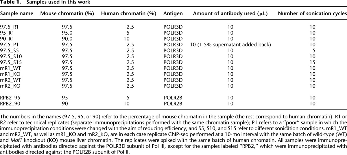
where the tilde symbol (∼) is used to refer to scores obtained after spike adjustment. The values are non-negative and can be used for analysis of relative occupancy in linear or log scale.

To obtain (log) ratios between the counts in the IP sample and in the input sample, we use the estimator:

where the pseudo counts (pc) are typically set to one but can be set higher to regularize ratios. In regions of high occupancy, is positive, whereas in regions where is very small or zero, the log ratio can be negative. These are the (log) scores we used in our analysis (Figs. 4–6).

Analysis method principle: sequencing depth and spike percentage

The calculation of the spike adjustment factor in Equation 6 is based on the mean of the sum of n signals in regions that, for us, correspond to annotated Pol III genes (whether or not occupied by Pol III) and other previously identified Pol III–occupied loci (Renaud et al. 2014). In principle, any set of known regions enriched in the factor of interest can be used. The efficiency of spike adjustment depends on sequencing depth and percentage of spike material. Here we make an estimate of the standard error of the adjustment factor considering the random variation of tag sampling. The adjustment factor is the ratio of the estimated means for the regions used (Equation 5). The sum of signals used for correction can be estimated as such: For the data in Figure 5, the sequencing depth is R ≈ 1.3 × 10⁸. The spike percentage is s = 2.5%, and signal content in the entire sample, computed for our set of 700 loci, is p ≈ 0.2%. Therefore, the total signal count sum is S = R × s × p ≈ 6500. Of the 700 human Pol III loci studied previously (Renaud et al. 2014), we singled out about 500 significantly occupied loci, which account for >90% of all Pol III loci counts (S ≈ 6000). The mean count per locus used for adjustment is thus about S/n ≈ 13, but it is the precision of S that determines the precision of the adjustment factor. Under the classic Poisson assumption for sampling error, the theoretical relative error r = sqrt(S)/S is about 0.013. For the adjustment factor, which is the ratio of two such quantities, the relative error is the double, thus ∼2.5%. To halve the theoretical relative error, one needs about four times more sequence tags, for example by increasing the proportion of the spike material to s = 10%. If there are more counts in known sites in the spike chromatin, say p = 10%, then one could reduce the spike chromatin percentage or sequence less deeply. Exact conditions need, however, to be determined for the specific parameters of each experiment.

Data analysis: tag alignment

The 100-nt sequence tags obtained after ultra-high-throughput sequencing were mapped onto the UCSC genome versions mentioned in Supplemental Tables S1, A and B, and S2, A and B, via the eland_extended mode of ELAND v2e in the Illumina CASSAVA pipeline v1.8.2. Only the tags with perfect matches, which represented >85% of the data, were kept for the analysis. Tags sequenced more than 50 times were given a maximum score of 50.

For the Pol III samples, counts were assigned to previously defined lists of human and mouse annotated Pol III genes and Pol III–occupied loci (Tables S2 and S3 in Renaud et al. 2014). For each locus the annotated RNA-coding region (e.g., tRNA) was extended by 150 bp on each side. One tag sequence was worth one count, and fractional counts were attributed in the case of a partial overlap between tag and locus. For the Pol II samples, tag counts were attributed in the same manner to regions extended by 250 bp on each side of the 22,572 annotated RefSeq TSSs (human), and on 11,217 annotated TSSs selected to be separated by at least 1000 bp from any other annotated TSS or polyadenylation site (mouse) (Le Martelot et al. 2012). The total numbers of tags, with and without redundancy, aligned onto the mouse and human genomes, as well as the numbers of tags falling in either mouse or human Pol III loci, are listed in Supplemental Tables S1, A and B, and S2, A and B.

Data analysis: normalization for sequencing depth

We normalized the mouse and human tags separately. We took the median of the total numbers of aligned tags across all the samples. We used this median as a reference total count. We then scaled bin counts in all samples to obtain a new total sample count equal to the reference total count. The typical reference total count was 150 million tags for mouse and 3 million for human tags. The input samples were normalized to the same total reference count as the ChIP samples.

Data analysis: calculating preliminary scores

For the Pol III data, we calculated scores as the non-negative residuals of the regression of ChIP bin counts versus input bin counts (see Equations 2–4). For the Pol II data, we calculated spp scores (Fig. 6). The regression coefficients from Equation 3 were estimated based on genomic bin counts outside of the regions being scored. For the Pol III experiments, we thus used a set of 400-bp bins covering the genome (6,637,291 bins on the mouse genome and 7,739,205 on the human genome). For the Pol II experiments, we used 500-bp bins (5,309,835 bins on the mouse genome and 6,191,402 on the human genome). We calculated tag counts for all bins, for ChIP and input samples. After selecting bins that did not overlap with the regions to be scored, we performed a robust linear regression on ChIP versus input. We used the regression coefficients to compute in regions to be scored. The values , which were background-adjusted, estimated the counts due to specific immunoprecipitation.

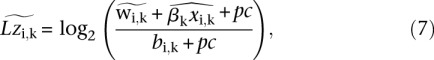
Data analysis: calculation of the spike adjustment factor and score adjustment

We used either a subset or all of the scored regions in the spike chromatin to calculate the score adjustment factor. Subselecting is inherent to our scoring method, since we select positive residuals only and set negative residuals to zero. Depending on the data analyzed, it might be appropriate to take upper quantiles or use a threshold score. The spike adjustment scaling (η) between two samples k and r was then computed as

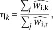where the ’s were the preliminary scores in the human regions j for these two samples. The index r here indicates a “reference” sample. The spike adjustment factor η was then applied as scaling factor to adjust the corresponding mouse gene scores: 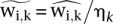. The example above considers the spike adjustment of one sample k with respect to a reference sample r. In practice, we adjusted multiple samples together. In our analysis and all figures, the reference was taken to be the mean of means of scores in all samples.

Data analysis: final scores for follow-up analysis

After spike adjustment, for final quantification we used the adjusted log ratios, as shown in Equation 7. The adjusted gene scores are still in linear scale. We re-added the estimated background and then took a log ratio with the observed background. These final scores were used in all figures in this manuscript.

Data access

The data from this study have been submitted to the NCBI Gene Expression Omnibus (GEO; http://www.ncbi.nlm.nih.gov/geo) under accession number GSE52049.

The CycliX Consortium

Nouria Hernandez,1 Mauro Delorenzi,2,3,4 Bart Deplancke,5 Béatrice Desvergne,1 Nicolas Guex,6 Winship Herr,1 Felix Naef,5 Jacques Rougemont,7 Ueli Schibler,8 Teemu Andersin,8 Pascal Cousin,1 Federica Gilardi,1 Pascal Gos,8 Fabienne Lammers,1 Sunil Raghav,5 Dominic Villeneuve,1 Roberto Fabbretti,6 Volker Vlegel,6 Ioannis Xenarios,1,2,6 Eugenia Migliavacca,1,6 Viviane Praz,1,2 Fabrice David,2,7 Yohan Jarosz,2,7 Dmitry Kuznetsov,6 Robin Liechti,6 Olivier Martin,6 Julien Delafontaine,2,7 Julia Cajan,5 Kyle Gustafson,1 Irina Krier,5 Marion Leleu,2,7 Nacho Molina,5 Aurélien Naldi,7 Leonor Rib,1 Laura Symul,5 and Gergana Bounova1,2

References

- Barski A, Cuddapah S, Cui K, Roh TY, Schones DE, Wang Z, Wei G, Chepelev I, Zhao K 2007. High-resolution profiling of histone methylations in the human genome. Cell 129: 823–837 [DOI] [PubMed] [Google Scholar]
- Canella D, Praz V, Reina JH, Cousin P, Hernandez N 2010. Defining the RNA polymerase III transcriptome: genome-wide localization of the RNA polymerase III transcription machinery in human cells. Genome Res 20: 710–721 [DOI] [PMC free article] [PubMed] [Google Scholar]
- Canella D, Bernasconi D, Gilardi F, LeMartelot G, Migliavacca E, Praz V, Cousin P, Delorenzi M, Hernandez N 2012. A multiplicity of factors contributes to selective RNA polymerase III occupancy of a subset of RNA polymerase III genes in mouse liver. Genome Res 22: 666–680 [DOI] [PMC free article] [PubMed] [Google Scholar]
- Chong SS, Hu P, Hernandez N 2001. Reconstitution of transcription from the human U6 small nuclear RNA promoter with eight recombinant polypeptides and a partially purified RNA polymerase III complex. J Biol Chem 276: 20727–20734 [DOI] [PubMed] [Google Scholar]
- Ciesla M, Boguta M 2008. Regulation of RNA polymerase III transcription by Maf1 protein. Acta Biochim Pol 55: 215–225 [PubMed] [Google Scholar]
- Desai N, Lee J, Upadhya R, Chu Y, Moir RD, Willis IM 2005. Two steps in Maf1-dependent repression of transcription by RNA polymerase III. J Biol Chem 280: 6455–6462 [DOI] [PubMed] [Google Scholar]
- Dhami P, Bruce AW, Jim JH, Dillon SC, Hall A, Cooper JL, Bonhoure N, Chiang K, Ellis PD, Langford C, et al. 2010. Genomic approaches uncover increasing complexities in the regulatory landscape at the human SCL (TAL1) locus. PLoS ONE 5: e9059. [DOI] [PMC free article] [PubMed] [Google Scholar]
- Enroth S, Andersson CR, Andersson R, Wadelius C, Gustafsson MG, Komorowski J 2012. A strand specific high resolution normalization method for chip-sequencing data employing multiple experimental control measurements. Algorithm Mol Biol 7: 2. [DOI] [PMC free article] [PubMed] [Google Scholar]
- Forsberg EC, Downs KM, Christensen HM, Im H, Nuzzi PA, Bresnick EH 2000. Developmentally dynamic histone acetylation pattern of a tissue-specific chromatin domain. Proc Natl Acad Sci 97: 14494–14499 [DOI] [PMC free article] [PubMed] [Google Scholar]
- Geiduschek EP, Kassavetis GA 2006. Transcription: adjusting to adversity by regulating RNA polymerase. Curr Biol 16: R849–R851 [DOI] [PubMed] [Google Scholar]
- Gjidoda A, Henry RW 2013. RNA polymerase III repression by the retinoblastoma tumor suppressor protein. Biochim Biophys Acta 1829: 385–392 [DOI] [PMC free article] [PubMed] [Google Scholar]
- Goodfellow SJ, White RJ 2007. Regulation of RNA polymerase III transcription during mammalian cell growth. Cell Cycle 6: 2323–2326 [DOI] [PubMed] [Google Scholar]
- Johnson DS, Mortazavi A, Myers RM, Wold B 2007a. Genome-wide mapping of in vivo protein–DNA interactions. Science 316: 1497–1502 [DOI] [PubMed] [Google Scholar]
- Johnson SS, Zhang C, Fromm J, Willis IM, Johnson DL 2007b. Mammalian Maf1 is a negative regulator of transcription by all three nuclear RNA polymerases. Mol Cell 26: 367–379 [DOI] [PubMed] [Google Scholar]
- Kharchenko PV, Tolstorukov MY, Park PJ 2008. Design and analysis of ChIP-seq experiments for DNA-binding proteins. Nat Biotechnol 26: 1351–1359 [DOI] [PMC free article] [PubMed] [Google Scholar]
- Landt SG, Marinov GK, Kundaje A, Kheradpour P, Pauli F, Batzoglou S, Bernstein BE, Bickel P, Brown JB, Cayting P, et al. 2012. ChIP-seq guidelines and practices of the ENCODE and modENCODE consortia. Genome Res 22: 1813–1831 [DOI] [PMC free article] [PubMed] [Google Scholar]
- Le Martelot G, Canella D, Symul L, Migliavacca E, Gilardi F, Liechti R, Martin O, Harshman K, Delorenzi M, Desvergne B, et al. 2012. Genome-wide RNA polymerase II profiles and RNA accumulation reveal kinetics of transcription and associated epigenetic changes during diurnal cycles. PLoS Biol 10: e1001442. [DOI] [PMC free article] [PubMed] [Google Scholar]
- Li QH, Brown JB, Huang HY, Bickel PJ 2011. Measuring reproducibility of high-throughput experiments. Ann Appl Stat 5: 1752–1779 [Google Scholar]
- Lin CY, Loven J, Rahl PB, Paranal RM, Burge CB, Bradner JE, Lee TI, Young RA 2012. Transcriptional amplification in tumor cells with elevated c-Myc. Cell 151: 56–67 [DOI] [PMC free article] [PubMed] [Google Scholar]
- Loven J, Orlando DA, Sigova AA, Lin CY, Rahl PB, Burge CB, Levens DL, Lee TI, Young RA 2012. Revisiting global gene expression analysis. Cell 151: 476–482 [DOI] [PMC free article] [PubMed] [Google Scholar]
- Mikkelsen TS, Ku M, Jaffe DB, Issac B, Lieberman E, Giannoukos G, Alvarez P, Brockman W, Kim TK, Koche RP, et al. 2007. Genome-wide maps of chromatin state in pluripotent and lineage-committed cells. Nature 448: 553–560 [DOI] [PMC free article] [PubMed] [Google Scholar]
- Nie Z, Hu G, Wei G, Cui K, Yamane A, Resch W, Wang R, Green DR, Tessarollo L, Casellas R, et al. 2012. c-Myc is a universal amplifier of expressed genes in lymphocytes and embryonic stem cells. Cell 151: 68–79 [DOI] [PMC free article] [PubMed] [Google Scholar]
- Oficjalska-Pham D, Harismendy O, Smagowicz WJ, Gonzalez de Peredo A, Boguta M, Sentenac A, Lefebvre O 2006. General repression of RNA polymerase III transcription is triggered by protein phosphatase type 2A-mediated dephosphorylation of Maf1. Mol Cell 22: 623–632 [DOI] [PubMed] [Google Scholar]
- Pluta K, Lefebvre O, Martin NC, Smagowicz WJ, Stanford DR, Ellis SR, Hopper AK, Sentenac A, Boguta M 2001. Maf1p, a negative effector of RNA polymerase III in Saccharomyces cerevisiae. Mol Cell Biol 21: 5031–5040 [DOI] [PMC free article] [PubMed] [Google Scholar]
- Rahl PB, Lin CY, Seila AC, Flynn RA, McCuine S, Burge CB, Sharp PA, Young RA 2010. c-Myc regulates transcriptional pause release. Cell 141: 432–445 [DOI] [PMC free article] [PubMed] [Google Scholar]
- Reina JH, Azzouz TN, Hernandez N 2006. Maf1, a new player in the regulation of human RNA polymerase III transcription. PLoS ONE 1: e134. [DOI] [PMC free article] [PubMed] [Google Scholar]
- Renaud M, Praz V, Vieu E, Florens L, Washburn MP, L’Hote P, Hernandez N 2014. Gene duplication and neofunctionalization: POLR3G and POLR3GL. Genome Res 24: 37–51 [DOI] [PMC free article] [PubMed] [Google Scholar]
- Ripperger J, Schibler U 2006. Rhythmic CLOCK-BMAL1 binding to multiple E-box motifs drives circadian Dbp transcription and chromatin transitions. Nat Genet 38: 369–374 [DOI] [PubMed] [Google Scholar]
- Roberts DN, Stewart AJ, Huff JT, Cairns BR 2003. The RNA polymerase III transcriptome revealed by genome-wide localization and activity-occupancy relationships. Proc Natl Acad Sci 100: 14695–14700 [DOI] [PMC free article] [PubMed] [Google Scholar]
- Roberts DN, Wilson B, Huff JT, Stewart AJ, Cairns BR 2006. Dephosphorylation and genome-wide association of Maf1 with Pol III-transcribed genes during repression. Mol Cell 22: 633–644 [DOI] [PMC free article] [PubMed] [Google Scholar]
- Rollins J, Veras I, Cabarcas S, Willis I, Schramm L 2007. Human Maf1 negatively regulates RNA polymerase III transcription via the TFIIB family members Brf1 and Brf2. Int J Biol Sci 3: 292–302 [DOI] [PMC free article] [PubMed] [Google Scholar]
- Upadhya R, Lee J, Willis IM 2002. Maf1 is an essential mediator of diverse signals that repress RNA polymerase III transcription. Mol Cell 10: 1489–1494 [DOI] [PubMed] [Google Scholar]
- Vannini A, Ringel R, Kusser AG, Berninghausen O, Kassavetis GA, Cramer P 2010. Molecular basis of RNA polymerase III transcription repression by Maf1. Cell 143: 59–70 [DOI] [PubMed] [Google Scholar]
- White RJ 2004. RNA polymerase III transcription and cancer. Oncogene 23: 3208–3216 [DOI] [PubMed] [Google Scholar]
- Willis IM, Moir RD 2007. Integration of nutritional and stress signaling pathways by Maf1. Trends Biochem Sci 32: 51–53 [DOI] [PubMed] [Google Scholar]