Automated detection of gastric slow wave events and estimation of propagation velocity vector fields from serosal high-resolution mapping

Abstract

High-resolution (HR; multi-electrode) recordings have led to detailed spatiotemporal descriptions of gastric slow wave activity. The large amount of data conveyed by the HR recordings demands an automated way of extracting the key measures such as activation times. In this study, a derivative-based method of identifying slow wave events was proposed. The raw signal was filtered using a second order Butterworth filter (low-pass; 10 Hz). The signal in each channel was differentiated and a threshold was taken as the 450% of the average of the negative first derivatives. An active event was defined where the first derivatives of the signal were more negative than the threshold. The accuracy of the method was validated against manually marked times, with a positive predictive value of 0.71. The detected activation times were interpolated using a second-order polynomial, the coefficients of which were evaluated using a previously developed least-square fitting method. The velocity fields were calculated, showing detailed spatiotemporal profile of slow wave propagation. The average of slow wave propagation velocity was 5.86 ± 0.07 mms⁻¹.

I. Introduction

Gastric motility is coordinated by an underlying electrical activity termed slow wave. It is now understood that slow waves are generated by the interstitial cells of Cajal in the stomach wall, and are passively conducted to the gastric smooth muscle cells [1], [2]. Dysrhythmic slow wave activity is thought to play an important role in common clinical conditions such as gastroparesis [3].

The use of high-resolution (HR) recording arrays is a key research tool in modern electrophysiology. The technique, when applied to the stomach, involves placing a spatially-dense array of electrodes directly over the serosal surface of the stomach, and simultaneously recording the resultant signals across multiple sites [4], [5]. HR recordings offer descriptions of both normal and abnormal slow waves at much greater spatiotemporal detail than the common method of suturing sparsely distributed electrodes along the greater curvature of the stomach. Recently, HR recording has also been employed to examine events underlying gastric slow wave dysrhythmias, revealing complex focal activities and waveform re-entry patterns not apparent in earlier studies employing fewer electrodes [6].

The main ways of identifying slow waves from a HR recording is through frequency characterization and activation maps [6]. The frequency can be determined efficiently from a fast Fourier transform of the signals to locating the dominant frequency in the frequency domain [7]. Activation maps are a graphical representation of the times at which the slow wave passes through each electrode. The time is commonly determined by the point of the most negative first derivative in a slow wave event [5]. Because HR recordings may yield a large amount of data in a short recording period, there is a need to automate the identification of slow wave activation times. Automatic identification has been previously attempted, however, virtually all previously described automated methods for slow waves were customized for the detection of bipolar signals from sparsely sutured serosal electrodes and are inappropriate for HR mapping techniques [8], [9]. Lammers et al. have proposed an automated algorithm for detection of slow wave events for unipolar HR recording, however the low perceived accuracy of this method has prevented it from being widely adopted to date [10]. New methods for the automated detection of slow wave activation times are therefore required.

The velocity of slow wave propagation should not be measured as a global value for the stomach, as the stomach exhibits clear difference in regional propagation behaviors as previously demonstrated in canine studies [11]. Traditionally, investigators have defined velocity as a vector quantity by either simply dividing the distance between two electrodes by the difference in the activation times between the slow waves, or via a finite-difference based derivative estimation from the neighboring 4 electrodes [4], [12]. The drawback with the neighboring electrodes approach, as Bayly et al. have pointed out, is that the direction of propagation must be accurately known before local velocity vector can be accurately evaluated [13]. Any deviations of time differences from the direction perpendicular to the wave-front may result in an error of estimating the velocity vector. Furthermore, velocity estimates from neighboring electrodes are prone to amplifying noise, particularly in HR mapping as velocity estimations are more sensitive to noise due to fine inter-electrode spacing.

In this study, an improved derivative-based method of automatically identifying slow wave events is presented, and validated using experimental recordings from a porcine model. A method of interpolating the activation times using previously-developed least-square-fitting algorithms, and velocity field calculations were also adapted for accurately representing slow wave characteristics in the porcine recordings.

II. RECORDING METHOD AND SIGNAL PROCESSING

A. Recording

Ethical approval for porcine experiments was obtained from the local institutional committee (The University of Auckland Animal Ethics Committee). The International Guiding Principles for Biomedical Research Involving Animals and Human Beings were followed. Recordings to validate the presented methods were performed in one female weaner cross-breed pig of weight 37.3 kg. The methods of anesthesia and surgery were as previously described [4]. An epoxy-embedded 48 channel electrode platform (4×12 array; inter-electrode distance 9 mm; silver electrodes) was positioned on the anterior porcine gastric corpus as shown in Fig. 1a. A five minute period of stabilization was allowed prior to a 15 minute recording period.

Fig. 1.

Recording setup. (a) the position of the electrode platform (4×12 electrodes; inter-electrode distance 9 mm). (b) a 60 s segment of recording from all 48 channels of the electrode platform (filtered via a second-order Butterworth filter with cut-off of 10 Hz).

All recordings were acquired using the Active Two System (Biosemi, Amsterdam). The common mode sense (reference) electrode was placed on the body surface of the lower abdomen, 5 cm below the incision. The right-leg drive electrode (ground) was placed on the right hind leg. The acquisition box was connected to a Dell M1450 notebook computer via a fiber-optic cable. The acquisition software was written in Labview 8.2 (National Instruments, Texas). The recording frequency was set to 512 Hz. The raw signal was filtered using a second-order Butterworth filter with a low-pass 10 Hz.

B. Post-processing

1) Manual marking

Manual marking was undertaken to develop a baseline standard to compare with the results of the automated detection method. Three markers with experience in recognizing serosal slow wave events marked a 180 s segment of the recording. Marking was done by importing the data segment into the SmoothMap software (www.smoothmap.org), and manually clicking on the electrograms on the graphical interface, where the marker identified a slow wave event to have occurred [14]. All markers marked the same segment of data independently from each other. Three separate lists of marked times were then compared and the following root-mean-square (RMS) measure (Equation 1) was used to calculate the error of each marker.

$$\epsilon =\sqrt{\frac{1}{m}\sum _{j=1}^m{(t_{ij}-\frac{1}{n}\sum _{i=1}^{n=3}{t}_{ij})}^2}$$ (1)

where i is the index of the number of markers (n = 3), and j is index of the same event that all the markers had marked an event within ± 500 ms. If one or more markers did not mark the same event, then that event was rejected from the calculation. The index of the total number of commonly marked events is denoted by m. The list of commonly marked events and their averaged times for each event was used as the baseline for quantifying the efficacy of the automated detection methods.

2) Derivative-based method

The automated detection algorithm for marking slow wave activation times is summarized in the following flowchart (Fig. 2),

Fig. 2.

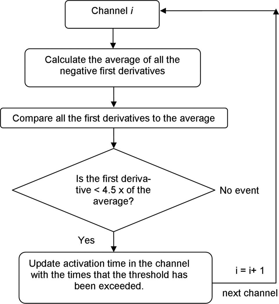
Slow wave event detection algorithm. The criteria for a positive event was that the first-derivative at that point is more negative than 4.5× the average of the negative first derivatives in that channel. The 4.5× threshold was determined to be the optimum value for detecting recordings by the E48 platform. Detection of slow waves was conducted in 15 s segments

3) Comparison method

The automatically marked slow wave events were compared to the reference times using the following equation,

$$\mathrm{\Delta }=\mathit{\text{min}}|t_{hk}-t_{hw}|,$$ (2)

$$t_{hk}=\frac{1}{n}\sum _{k=1}^m{t}_{hk}$$ (3)

where t_hk is the average of the k^th manually marked events in channel h, and t_hw is the w^th automatically marked event also in the same h^th channel. The detected events were compared to all the reference events once, and if the minimum error was within ± 500 ms then the automatically detected event was defined as a true positive (TP) event, out of the total number of manually detected events (P). The remaining detected events by the algorithm were designated false positive (FP). The number of reference events that the algorithm had missed was designated false negative (FN). In addition, the positive predictive value (PPV) was also calculated using the following equation,

$$PPV=\frac{TP}{TP+FP}$$ (4)

Velocity Calculation: The velocity calculation method was adapted from the algorithms developed by Bayly et al. [13]. In order to calculate a uniform spatially-distributed velocity field, the activation times from each wave were first interpolated using the following second-order polynomial,

$$T(x,y)=p(1)x^2+p(2)y^2+p(3)xy+p(4)x+p(5)y+p(6)$$ (5)

where T(x, y) is the interpolated activation times at location x and y in the electrode array. The array of p contains six coefficients for the second-order polynomial. A previously developed least-square-fitting algorithm (Equation 6–7) was used to calculate the polynomial coefficients [13].

$$Ap=\left[\begin{array}{c}\hfill t_1\hfill \\ \hfill ·\hfill \\ \hfill ·\hfill \\ \hfill ·\hfill \\ \hfill ·\hfill \\ \hfill t_n\hfill \end{array}\right]=\left[\begin{array}{cccccc}\hfill x_1^2\hfill & \hfill y_1^2\hfill & \hfill x_1{y}_1\hfill & \hfill x_1\hfill & \hfill y_1\hfill & \hfill 1\hfill \\ \hfill ·\hfill & \hfill ·\hfill & \hfill ·\hfill & \hfill ·\hfill & \hfill ·\hfill & \hfill ·\hfill \\ \hfill ·\hfill & \hfill ·\hfill & \hfill ·\hfill & \hfill ·\hfill & \hfill ·\hfill & \hfill ·\hfill \\ \hfill ·\hfill & \hfill ·\hfill & \hfill ·\hfill & \hfill ·\hfill & \hfill ·\hfill & \hfill ·\hfill \\ \hfill ·\hfill & \hfill ·\hfill & \hfill ·\hfill & \hfill ·\hfill & \hfill ·\hfill & \hfill ·\hfill \\ \hfill x_n^2\hfill & \hfill y_n^2\hfill & \hfill x_n{y}_n\hfill & \hfill x_n\hfill & \hfill y_n\hfill & \hfill 1\hfill \end{array}\right]\left[\begin{array}{c}\hfill p_1\hfill \\ \hfill p_2\hfill \\ \hfill p_3\hfill \\ \hfill p_4\hfill \\ \hfill p_5\hfill \\ \hfill p_6\hfill \end{array}\right]$$ (6)

The polynomial coefficient (p) was solved by

$$p=V{S}^{-1}{U}^{T}t$$ (7)

where t is the automatically identified activation times of slow wave events. Matrix A contains evaluated terms using the x and y coordinates of the corresponding activation time. For solution for p was solved by using the singular value decomposition of A into V, S, and U (A = USV^T). The search parameters for the number of events included in one wave were over the entire set of electrodes (Δ x = 99 mm; Δ y = 27 mm) within a 10 s interval (Δ t = 10 s). For the description of normal events, the number of active electrodes within the 4×12 array was adequately fitted by a second-order polynomial due to the slow moving wave front of the gastric slow waves.

Velocity was calculated using the following equation,

$$V(x,y)=\left[\begin{array}{c}\hfill \frac{\partial x}{\partial t}\hfill \\ \hfill \frac{\partial x}{\partial t}\hfill \end{array}\right]=\left[\begin{array}{c}\hfill \frac{T_x}{T_x^2+T_y^2}\hfill \\ \hfill \frac{T_y}{T_x^2+T_y^2}\hfill \end{array}\right],T_x=\frac{\partial T}{\partial x},T_y=\frac{\partial T}{\partial y}$$ (8)

where V (x, y) is the velocity vector evaluated at coordinates x and y on the electrode array.

III. RESULTS AND DISCUSSION

There was some variation in the accuracy of the manually marked slow wave events between markers, as shown in Table I. The maximum RMS error was 111 ms and minimum RMS error was 82 ms, both of which were in the acceptable deviation (± 500 ms) as previously defined in the method section. The markers spent an average of 11.2 min to mark all the slow wave events in the 180 s segment. Furthermore, all markers had also identified events that were not also marked by the other markers, resulting in an inconsistency in the total number of slow wave events marked by each marker. Based on the marked events the intrinsic frequency of slow waves was 2.65 cycles per minute (cpm).

TABLE I.

Variation between the manually marked slow wave events of individual markers.

E48(252)	M1	M2	M3
Time taken (min)	10	10	14
events	287	257	255
RMS error (ms)	85	111	82

The derivative-based algorithm demonstrated a reasonable agreement with the manually marked times (Table II). The algorithm identified 230 true positive events out of the potential 252 positive events identified manually (PPV 0.71). Given that the algorithm did not require strenuous pre-processing steps, the PPV of 0.71 was fairly high. The algorithm compared favourably with a previously published agorithm [5], which achieved a PPV of 0.62. Tests conducted across multiple segments of recordings using the E48 platform showed a relatively stable performance (PPV 0.71 – 0.97).

TABLE II.

Accuracy of the derivative-based identification method

Derivative-based method	accuracy measure
True positive	230
False positive	94
False negative	22
Positive predictive value	0.71

The automatically identified slow wave activation times (Fig. 3a) and interpolated activation times (Fig. 3b) for the first two waves analyzed showed reasonable agreement. The interpolated times were calculated over 10 points in each direction, and the spatial regularity of the interpolated activation times allowed easier construction of activation maps of the first wave (Fig. 3c) and the second wave (Fig. 3d), both of which showed a consistent origin and direction of slow wave propagation.

Fig. 3.

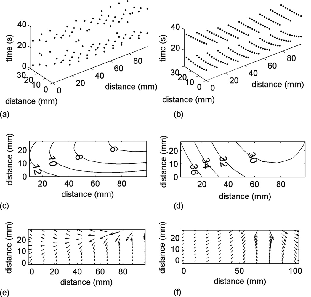
Slow wave detection, interpolation, activation mapping and velocity field calculation. (a) automatically detected slow wave events over the first 2 waves; (b) interpolated activation times over the first 2 waves; (c) activation map (labeled in seconds) of the first wave; (d) activation map (labeled in seconds) of the second wave; (e) velocity field of the first wave; (f) velocity field of the second wave.

Equation 7 was used to calculate the velocity for the first wave (Fig. 3e) and the second wave (Fig. 3f), both of which clearly demonstrate that there was a localized pattern of high velocity propagation near the origin of slow wave activity recorded by the platform. The average velocity was 5.86 ± 0.07 mms⁻¹. However, it should be noted that there was a clear spatial distribution of velocity profile in each wave of slow waves as shown in Fig. 3e and Fig. 3f.

IV. CONCLUSIONS

A derivative-based method was developed to automatically identify porcine gastric slow wave activation times. The algorithm had a positive-predictive value of 0.71 relative to a set of manually identified slow waves. The new method improved upon previous methods because a threshold for locating slow wave was assigned to each channel. Given the variation in slow wave amplitudes across the stomach [6], this method presents an efficient way of processing HR recording; A second-order polynomial was fitted over the detected activation times using a previously developed least square fitting method [13]. The velocity field was calculated for consecutive cycles of slow wave events based on the interpolated activation times to reduce the effects of outliers in marked slow wave events. The average of slow wave propagation velocity was 5.86 ± 0.07 mms⁻¹.

REFERENCES

- 1.Sanders KM. A case for interstitial cells of Cajal as pacemakers and mediators of neurotransmission in the gastrointestinal tract. Gastroenterology. 1996;111(2):492–515. doi: 10.1053/gast.1996.v111.pm8690216. [DOI] [PubMed] [Google Scholar]
- 2.Cheng LK, O’Grady G, Du P, Egbuji JU, Windsor JA, Pullan AJ. Gastrointestinal system. Wiley Interdiscip Rev Syst Biol Med. 2010 Jan-Feb;2(1):65–79. doi: 10.1002/wsbm.19. [DOI] [PMC free article] [PubMed] [Google Scholar]
- 3.Chen JDZ, Pan LJ, McCallum RW. Abnormal gastric myoelectrical activity and delayed gastric emptying in patients with symptoms suggestive of gastroparesis. Dig. Dis. Sci. 1996;41:1538–1545. doi: 10.1007/BF02087897. [DOI] [PubMed] [Google Scholar]
- 4.Du P, O’Grady G, Egbuji JU, Lammers WJ, Budgett D, Nielsen P, Windsor JA, Pullan AJ, Cheng LK. High-resolution mapping of in vivo gastrointestinal slow wave activity using flexible printed circuit board electrodes: methodology and validation. Ann Biomed Eng. 2009 Apr;37(4):839–846. doi: 10.1007/s10439-009-9654-9. [DOI] [PMC free article] [PubMed] [Google Scholar]
- 5.Lammers WJ, Al-Kais A, Singh S, Arafat K, El-Sharkawy TY. Multielectrode mapping of slow-wave activity in the isolated rabbit duodenum. J Appl Physiol. 1993;74(3):1454–1461. doi: 10.1152/jappl.1993.74.3.1454. [DOI] [PubMed] [Google Scholar]
- 6.Lammers WJ, Ver Donck L, Stephen B, Smets D, Schuurkes JA. Focal Activities and Re-Entrant Propagations as Mechanisms of Gastric Tachyarrhythmias. Gastroenterology. 2008 doi: 10.1053/j.gastro.2008.07.020. [DOI] [PubMed] [Google Scholar]
- 7.Buist ML, Cheng LK, Sanders KM, Pullan AJ. Multiscale modelling of human gastric electric activity: can the electrogastrogram detect functional electrical uncoupling? Exp Physiol. 2006;91(2):383–390. doi: 10.1113/expphysiol.2005.031021. [DOI] [PubMed] [Google Scholar]
- 8.Chen JZ, Zou X, Lin X, Ouyang S, Liang J. Detection of gastric slow wave propagation from the cutaneous electrogastrogram. Am J Physiol. 1999;277:G424–G430. doi: 10.1152/ajpgi.1999.277.2.G424. [DOI] [PubMed] [Google Scholar]
- 9.Wang ZS, Elsenbruch S, ORR WC, Chen JZ. Detection of gastric slow wave uncoupling from multi-channel electrogastrogram: validations and applications. Neurogastroenterol Motil. 2003;15:457–465. doi: 10.1046/j.1365-2982.2003.00430.x. [DOI] [PubMed] [Google Scholar]
- 10.Lammers WJ, Michiels B, Veoten J, Ver Donck L, Schuurkes JA. Mapping slow waves and spikes in chronically instrumented conscious dogs: automated on-line electrogram analysis. Med Biol Eng Comput. 2008 Feb;46(2):121–129. doi: 10.1007/s11517-007-0294-7. [DOI] [PubMed] [Google Scholar]
- 11.Kelly KA, Code CF, Elveback LR. Patterns of canine gastric electrical activity. Am J Physiol. 1969;217:461–470. doi: 10.1152/ajplegacy.1969.217.2.461. [DOI] [PubMed] [Google Scholar]
- 12.Lammers WJ, Ver Donck L, Schuurkes JA, Stephen B. Peripheral pacemakers and patterns of slow wave propagation in the canine small intestine in vivo. Can J Physiol Pharmacol. 2005;83(11):1031–1043. doi: 10.1139/y05-084. [DOI] [PubMed] [Google Scholar]
- 13.Bayly PV, KenKnight BH, Rogers JM, Hillsley RE, Ideker RE, Smith WM. Estimation of conduction velocity vector fields from epicardial mapping data. IEEE Trans Biomed Eng. 1998 May;45(5):563–571. doi: 10.1109/10.668746. [DOI] [PubMed] [Google Scholar]
- 14.Lammers WJ. www.smoothmap.org. [Google Scholar]