Abstract
Summary: The Dirichlet-multinomial (DMN) distribution is a fundamental model for multicategory count data with overdispersion. This distribution has many uses in bioinformatics including applications to metagenomics data, transctriptomics and alternative splicing. The DMN distribution reduces to the multinomial distribution when the overdispersion parameter ψ is 0. Unfortunately, numerical computation of the DMN log-likelihood function by conventional methods results in instability in the neighborhood of  . An alternative formulation circumvents this instability, but it leads to long runtimes that make it impractical for large count data common in bioinformatics. We have developed a new method for computation of the DMN log-likelihood to solve the instability problem without incurring long runtimes. The new approach is composed of a novel formula and an algorithm to extend its applicability. Our numerical experiments show that this new method both improves the accuracy of log-likelihood evaluation and the runtime by several orders of magnitude, especially in high-count data situations that are common in deep sequencing data. Using real metagenomic data, our method achieves manyfold runtime improvement. Our method increases the feasibility of using the DMN distribution to model many high-throughput problems in bioinformatics. We have included in our work an R package giving access to this method and a vingette applying this approach to metagenomic data.
Availability and implementation: An implementation of the algorithm together with a vignette describing its use is available in Supplementary data.
Contact: pengyu.bio@gmail.com or cashaw@bcm.edu
Supplementary information: Supplementary data are available at Bioinformatics online.
1 INTRODUCTION
The analysis of count data (Cameron and Trivedi, 2013; Winkelmann, 2008) or categorical data (Agresti, 2002) is an important topic in statistics and has a wide variety of applications in bioinformatics. The advent of high-throughput sequencing technologies (Metzker, 2010) provides unprecedented opportunities for investigating new and more powerful analysis methods on count data (Anders and Huber, 2010; Robinson et al., 2010).
The Poisson distribution is a basic distribution for modeling count data. An important property of the Poisson distribution is that the mean and variance are the same, which is called equidispersion. However, the mean and the variance of real count data are often not the same; in fact, the variance is often greater than the mean. This makes the Poisson distribution not ideal for analyzing such data because the equidispersion assumption is violated. The phenomenon where a dataset exhibits greater variance than what would be expected in a statistical model is called overdispersion. A commonly used overdispersed model for the Poisson distribution is the negative-binomial distribution. This distribution has been extensively studied in Hilbe (2011) and is an indispensable model for high-throughput sequencing data (Anders and Huber, 2010).
Another fundamental model in count data analysis is the multinomial (MN) distribution, which is useful for analysis of count proportions among multiple categories. One important use case of the MN distribution is Fisher’s exact test of contingency tables (Fisher, 1973; Mehta and Patel, 1986), which has been used in the analysis of alternative 3′ UTR utilization (Wan, 2012) and splicing (Lu et al., 2013), as well as metagenomics (Gomez-Alvarez et al., 2012). In the regression context, MN logistic regression is also commonly used (Agresti, 2002). However, real data often exhibit heterogeneity that is usually thought to be caused by dependencies or the similarity of responses of members of the same cluster in cluster sampling (Brier, 1980). This leads to extra-multinomial variation (Haseman and Kupper, 1979), i.e. overdispersion with respect to the MN distribution.
The modeling of overdispersion of the MN distribution has been addressed by extending the MN distribution to the Dirichlet-multinomial (DMN) distribution (Mosimann, 1962; Poortema, 1999). The beta-binomial (BB) distribution—a special case of the DMN distribution with only two categories—has been studied by many (Crowder, 1978; Kleinman, 1973; Skellam, 1948). Because of its flexibility and its mathematical convenience, the DMN distribution is widely applied to diverse fields, such as topic modeling (Mimno and McCallum, 2008), magazine exposure modeling (Leckenby and Kishi, 1984; Rust and Leone, 1984), word burstiness modeling (Madsen et al., 2005), language modeling and (MacKay and Bauman Peto, 1994) multiple sequence alignment (Brown et al., 1993; Sjölander et al., 1996). Bouguila (2008) also considered a generalization of the DMN distribution and applied it to count data clustering. Another related distribution for handling overdispersion is the Dirichlet negative MN distribution (Mosimann, 1963) allowing the modeling of correlated count data without an upper bound, which has many possible uses in biostatistics and bioinformatics (Farewell and Farewell, 2013).
Likelihood functions play a key role in statistical inference (Casella and Berger, 2002). For example, likelihood functions can be used for parameter estimation, hypothesis testing and interval estimation. In the context of the DMN distribution, there has been recent research to investigate the Fisher information matrix (Paul et al., 2005) and maximum likelihood estimation (MLE) (Neerchal and Morel, 2005). Not all statistical inference methods are based on likelihood functions. For instance Kim and Margolin (1992) developed a method for testing the goodness of fit of the MN distribution against the DMN distribution based on the  test statistic (Tarone, 1979), a flexible framework built on the likelihood approach that enables the analysis of complex experimental designs (McCullagh and Nelder, 1989) that frequently appear in genomic and bioinformatics studies.
In this article, we study the fundamental problem of the evaluation of the DMN log-likelihood function. In Section 2, we demonstrate the instability and runtime problems of two existing methods for computing the DMN log-likelihood function and propose a novel parameterization of the log-likelihood function to allow smooth transition from the overdispersed case (the DMN distribution) to the non-overdispersed case (the MN distribution). For this new parameterized form, in Section 3 we introduce a new formula based on a truncated series consisting of Bernoulli polynomials. In Section 4, a mesh algorithm is devised to increase the applicability of this new formula. In Section 5, we show numerical results of the mesh algorithm, confirm its stability and runtime improvements. Finally, we applied our method to human microbiome data and demonstrated its large performance improvement over the most accurate existing method.
2 DMN DISTRIBUTION
The DMN distribution, a.k.a., the compound MN distribution (Mosimann, 1962), is an extension of the MN distribution. The probability mass function (PMF) of the K categories MN distribution of N-independent trials is given by
| (1) |
where  denotes the factorial of a non-negative integer n; the observations
  , satisfying
  , are non-negative integers; and
  , satisfying
  , are the probabilities that these K categories occur.
The DMN distribution can be generated if the probabilities  follow a prior distribution (of the positive parameters
  ) conjugate to the PMF
  (Bishop, 2006)
This distribution is called the Dirichlet distribution whose normalized form is
 |
(2) |
where  is the gamma function and
  .
.
The PMF of the DMN distribution is derived by taking the integral of the product of the Dirichlet prior (2) and the MN likelihood (1) with respect to the probabilities  (Mosimann, 1962),
 |
(3) |
where, same as the MN distribution,  are non-negative integers, satisfying
  . The DMN distribution reduces to the BB distribution when there are only two categories (K = 2).
The first term on the right side of (3) does not depend on the parameter  . For common uses of the likelihood function in statistics, e.g. in the maximum-likelihood estimation, we are not interested in the first term but in the product of the remaining two terms, i.e. we are interested in the last two terms of the DMN likelihood function in (3)
| (4) |
By taking the logarithm of both sizes of (4), we get the log-likelihood function
 |
(5) |
When  , it can be shown that the DMN distribution is reduced to the MN distribution. As
  becomes 0 under this limit, it is convenient to use the parameter ψ instead of A.
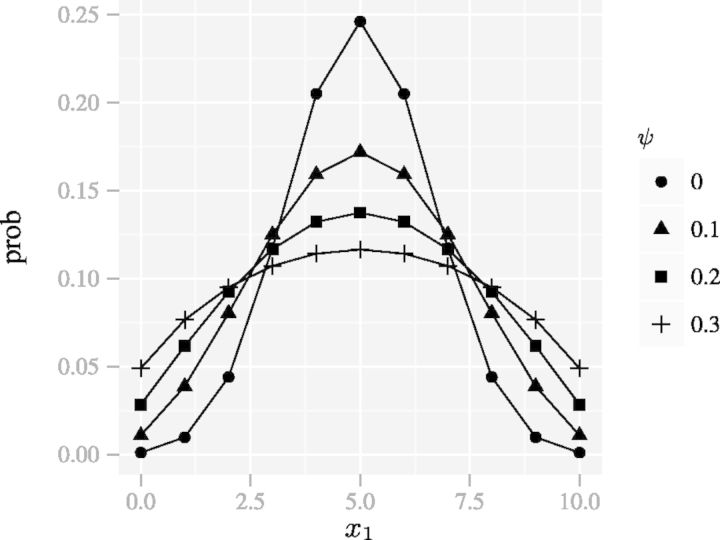
The parameter ψ characterizes how different a DMN distribution is from the corresponding MN distribution with the same category probabilities. The greater the parameter ψ, the greater the difference. This additional parameter gives the DMN distribution the ability to capture variation that cannot be accommodated by the MN distribution. We call ψ the overdispersion parameter in this article, with the understanding that the greater the ψ, the greater the variance. As an example, Figure 1 shows that increasing the dispersion parameter ψ of the BB dispersion increases the variance of the count of the first category x1. Using  , (5) becomes
 |
(6) |
where  . One shortcoming of (6) is that it is undefined for
  . Hence, R (R Core Team, 2013) functions implementing (6), such as dirmult () from dirmult (Tvedebrink, 2009) and betabin () from aod (Lesnoff and Lancelot, 2012), return NaN when
  . Another shortcoming of (6) is that as
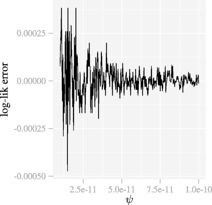
  the function implementing (6) is unstable as shown in Figure 2.
Fig. 1.
The PMFs of a family of the BB distributions (N = 10) with different dispersion parameters ψ. The spread of the distributions increases with the dispersion parameter, whereas the mean remains constant
Fig. 2.
The function implementing (6) is unstable when ψ approaches 0. The parameters are  and
and 
Alternatively, the likelihood representation used in the method in the R package VGAM (Yee, 2010, 2012; Yee and Wild, 1996), (4) can be written as
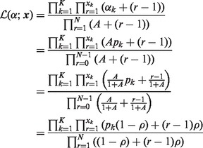 |
where  is the overdispersion parameter defined therein, which is different from our definition of the overdispersion parameter ψ in (6). The log-likelihood function can be written as
 |
(7) |
When there is 0 overdispersion ( ), (7) reduces to the MN log-likelihood and it is numerically stable when
  . But the number of terms on the right side of (7) is proportional to N. When N is large, the runtime is long.
3 APPROXIMATION OF PAIRED LOG-GAMMA DIFFERENCE
We see that (6) consists of paired  differences, such as
  . When ψ is close to 0, each
  term becomes exceedingly large, but the paired differences become relatively small. Because of the limited precision of the floating-point arithmetic (IEEE Task P754, 2008), the large terms cancel and the result is left with large errors. We solve this large error problem by a new approximation to the
  difference. Let us consider
  and
and  . Rowe (1931) showed that
  (z and a are complex numbers) can be asymptotically expanded as
 |
(8) |
where  denotes the nth Bernoulli polynomial. The term
  means that, for any fixed m, the error of the right side of (8) (with the term
  removed) as an approximation to
  is bounded by
  times some constant as
  . Let a = 0,
 |
where Bn denotes the nth Bernoulli number ( ). Let
  and a = y, the difference between the above two equations is
 |
(9) |
where
| (10) |
is the old type Bernoulli polynomial (Whittaker and Watson, 1927). The infinite series
| (11) |
converges absolutely when y is an integer and  (Freitag and Busam, 2009). Note that x = 0 is a removable singularity of
 . Using the properties of analytic functions, we have (Freitag and Busam, 2009)
| (12) |
Therefore, for any integer y, we can use the following approximation
| (13) |
when y is an integer and  and
and
| (14) |
The error is bounded by
| (15) |
if  , where δ is a constant <1. For the application of computing the DMN log-likelihood function, we have
  and
and  . So we instead require
| (16) |
for simplicity.
The error bound (15) can be arbitrarily small for arbitrarily large m without considering the numerical errors in computing the Bernoulli polynomials  . In practice, high order polynomials are difficult to compute using floating-point arithmetic (Lauter and Dinechin, 2008). Because the subscript n equals the order of the Bernoulli polynomial
  , if m is too large, the error of each terms of
  may actually be large, which makes
  inaccurate. Hence, we do not want too many terms in (14). So we choose m = 20 such that
  (
( ) are still numerically accurate. We also do not need the error bound (15) to be smaller than the machine epsilon of the double precision data type (
 ). Therefore, we choose
  , which leads to an error bound of ∼
 , which is a little less than the machine epsilon.
4 THE MESH ALGORITHM FOR COMPUTING THE DMN LOG-LIKELIHOOD
We apply (13) to compute the DMN log-likelihood function (6). To cope with the requirement (16), by using the idea of analytic continuation (Freitag and Busam, 2009), we introduce a mesh algorithm and allow the computation of the DMN log-likelihood using the approximation (13) in the whole parameter domain of the DMN log-likelihood function. First, we study  in (6) in detail. Let
  be the vector of the non-zero elements in
  ,
,  be a vector of the corresponding elements in
  and
and  be the length of
  , then (6) becomes
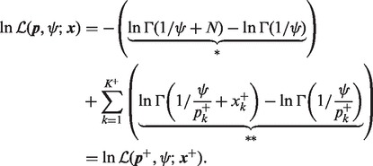 |
(17) |
When
| (18) |
after taking the sum over k on both sides, we have
 |
(19) |
Therefore, the (*) term and all the  (**) terms in (17) meet the condition (16). Then the approximation (13) can be used for all
  paired
  differences in (17),
 |
(20) |
When some of the  (**) terms in (17) do not meet the condition (18), we can rewrite the vector
  into the sum of L terms choosing the terms to meet this condition
| (21) |
We describe the choice of  below. For convenience, we define
 |
(22) |
Note that we have the following relation between the adjacent  ’s,
’s,
| (23) |
or
| (24) |
By taking the sum of all the elements in each vector in (22), we have
 |
(25) |
where  and
and  . Or we write it as
| (26) |
Strictly speaking, (25) is undefined for  , but when
  , all
, all  should be 0 s. To make (25) numerically valid for all
  , we write
 |
(27) |
Similarly, for  , we have
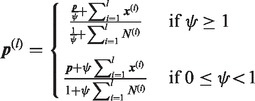 |
(28) |
Then, using (24) and (26), (6) can be broken into a sum of L log-likelihoods,
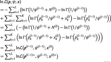 |
(29) |
The sum in (29) is used in our algorithm to evaluate the log-likelihood function. We can always increase L and set  intelligently, so that the condition (16) is satisfied for all the terms in the last formula in (29). In this case, each of the L terms in (29) can be computed using (20). This means that the log-likelihood function
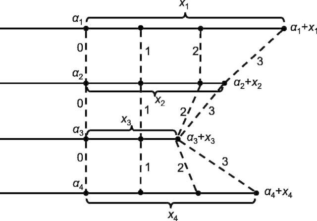
  can be evaluated incrementally on a mesh (Fig. 3). Hence, we name this method the mesh algorithm. Note that there can be many ways to generate the mesh. We describe below how the mesh is generated in our implementation. We first create an initial mesh with the following scheme
| (30) |
where  denotes the floor function. The level of mesh L is chosen so that it is the smallest integer satisfying
| (31) |
Fig. 3.
A graphical depiction of the mesh algorithm for evaluation of the log-likelihood in (29). The count in the ith category is represented by a line segment and can be partitioned into a sum of L = 3 sub-counts represented by sub-segments. At points connected by the dashed lines ( ), the DMN log-likelihood can be evaluated using (20), and there are three such evaluations in this example
This initial mesh needs to be adjusted because the end of the mesh should total to match xi exactly. To do so, let  be the smallest number satisfying
 |
(32) |
We adjust  so that
  . For each i, all the remaining
  (
( ) are set to 0. With this adjusted mesh, we can use the approximation (20) to compute the DMN log-likelihood (29). Figure 3 shows an example with L = 3. The 3 segments of x2 is 0; hence, there are only two non-zero segments as shown. x1, x3 and x4 are broken into three non-zero segments. The last non-zero segments of all the four lines are adjusted so the segment sums equal xi (
 ), respectively.
Note that the time complexity of the mesh algorithm is proportional to  , which is smaller than
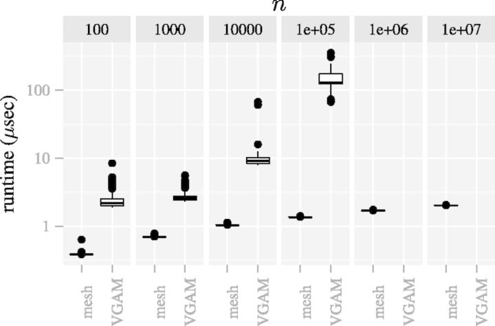
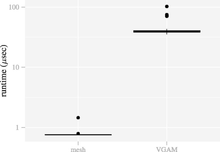
  , the time complexity of (7) (VGAM). The difference becomes especially prominent for high count data (Figs 6 and 8).
Fig. 6.
The mesh algorithm is much faster than the algorithm in VGAM for the DMN log-likelihood computation. The parameters are  ,
,  and
and  . The computation using VGAM is only up to
  , as it takes too much runtime when n is beyond this point. Each boxplot represents 100 DMN log-likelihood evaluations
Fig. 8.
The mesh algorithm is much faster than the algorithm in VGAM on the saliva dataset. The parameters are  , 0.147, 0.117, 0.088, 0.065, 0.054, 0.041, 0.033, 0.026, 0.022, 0.019, 0.017, 0.015, 0.014, 0.012, 0.011, 0.009, 0.009, 0.008, 0.007, 0.090) and
5 THE NUMERICAL RESULTS
We implemented the mesh algorithm for computing the DMN log-likelihood in C++. In this section, we demonstrate the accuracy and runtime of the mesh algorithm. All experiments were run on a Linux machine with a 4-core Intel Xeon CPUs E5630@ 3.53 GHz. Each log-likelihood function call is single-threaded.
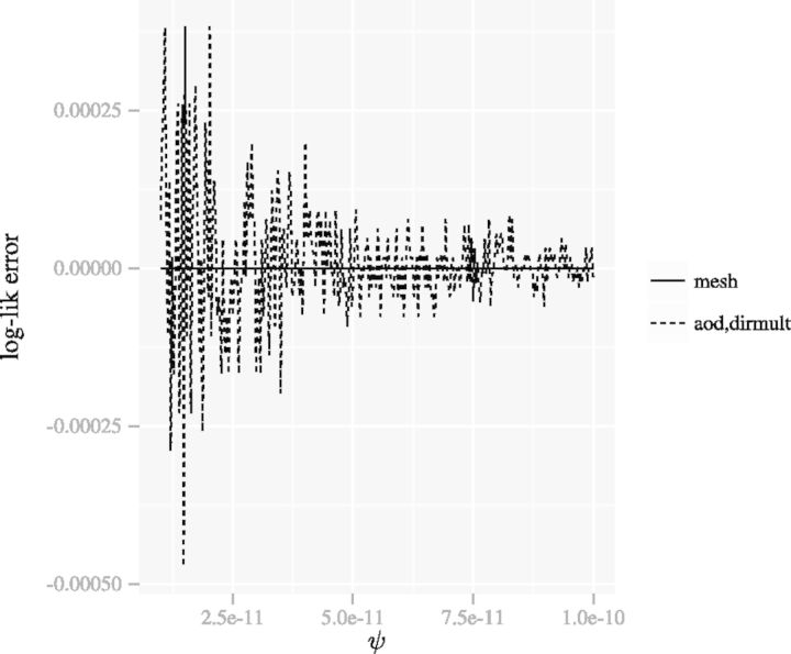
In contrast to Figure 2, Figure 4 shows that the mesh algorithm is numerically stable when ψ approaches 0.
Fig. 4.
The figure presents a comparison of methods for evaluation of the DMN log-likelihood function when the dispersion parameter ψ varies. For the mesh algorithm, the evaluation is accurate and stable when the dispersion parameter ψ approaches 0. The aod(dirmult) algorithm is unstable. The parameters are  and
and 
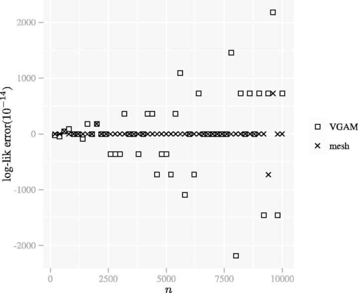
We compute the error of the mesh algorithm by comparing its results with the results of an implementation of (4) in Sage (Stein et al., 2012), which can achieve arbitrarily high accuracy. Figure 5 compares the error of the mesh algorithm and the error of the method in VGAM. We can see the mesh algorithm is more accurate.
Fig. 5.
The error of the mesh algorithm is smaller than the error of the method in VGAM. The error of the aod(dirmult) algorithm is larger than the scale presented. The parameters are  ,
,  and
and 
Figure 6 shows that the runtime of the mesh algorithm increases more slowly as the counts n increase than the method in VGAM. Note that only R code is used to implement the method in VGAM, whose speed can be improved by using C++. However, its runtime scalability with respect to the parameter n is intrinsic to the representation of the log-likelihood function (7) and independent of the implementation. The slower increase of runtime is especially important for the high count that is typical in contemporary high-throughput sequencing datasets.
6 BIOINFORMATICS APPLICATION
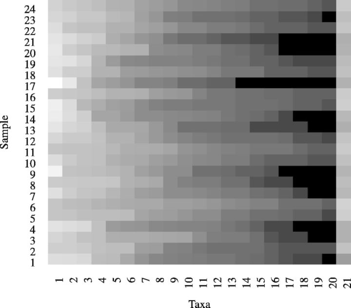
We demonstrate below the application of our new method in analyzing human microbiome data from the Human Microbiome Project clinical production pilot study (The NCBI BioProject website, 2010). This dataset consists of the pyrosequencing of 16S rRNA genes in samples from four body sites, namely, saliva, throat, tongue and palatine tonsil of 24 human subjects (Rosa et al., 2013). The sequences obtained from the V1–V3 and V3–V5 variable regions of the 16 S ribosomal RNA gene are classified into the 20 most abundant taxa at the genus level and the remaining sequences are classified as the 21st taxa (La Rosa et al., 2012). Figure 7 shows the taxa distribution with each sample of the saliva dataset.
Fig. 7.
The heatmap of the saliva 16 S rRNA pyrosequencing dataset. Each row represents a sample and each column represents a taxa. The brighter the color, the higher the proportion of the taxa within the sample
On real datasets, the mesh algorithm is much faster than the algorithm in VGAM. For example, the mesh algorithm improves the speed by over  on the saliva dataset (Fig. 8).
Because the  -based test (Kim and Margolin, 1992) rejects the hypothesis that the data from any of the four body sites are distributed according to the MN distribution (the P-values are 0 for all the four body sites), we use the DMN distribution to model each of the four datasets. Table 1 shows the maximum likelihood estimates of the dispersion parameters ψ for the data from all four body sites.
Table 1.
The MLE of the dispersion parameters of the 16S rRNA pyrosequencing data from all four body sites
| Body site | ψ |
|---|---|
| Saliva | 0.00389 |
| Throat | 0.00639 |
| Tongue | 0.00802 |
| Tonsils | 0.01039 |
7 DISCUSSION
Overdispersion is important and needs to be accommodated in modeling count data. To handle overdispersion in MN data, the DMN distribution is commonly used. The numerical computation of the log-likelihood function is important for performing statistical inference using this distribution. Previous work has provided useful methods for this calculation, but the requirements of bioinformatics are difficult to satisfy. Our method solves the accuracy and runtime challenges.
Overdispersion is commonly found in high-throughput sequencing data. The overdispersed Poisson model (the negative-binomial distribution) has been used to detect differential gene expression. However, the DMN distribution has seen limited use in analyzing high-throughput sequencing data, possibly because the existing methods based on the DMN distribution did not anticipate the high counts and the vast amount of such count tables extracted from the high-throughput sequencing technologies.
To overcome the instability problem and the runtime problem of the existing methods for computing the log-likelihood, we derived a new approximation of the DMN log-likelihood function based on Bernoulli polynomials. Using a novel mesh algorithm, we are able to compute the log-likelihood for any parameters in the domains of the log-likelihood function. Comparing with the existing methods, the mesh algorithm is more accurate and is much faster. We demonstrate the application of the new method in analyzing human microbiome data with a large runtime improvement. This method is generally applicable to other scenarios involving proportions, such as alternative exon utilization (Wang et al., 2008) and alternative poly-A utilization (Lutz and Moreira, 2011). For example, suppose we have 10 000 alternative splicing events that need to be tested and each test requires 1000 log-likelihood function evaluations. Our method can reduce the runtime to hours instead of potentially days. This work paves the way for application of the DMN distribution to model overdispersion in large-scale count data available in the high-throughput sequencing era.
Funding: This work was supported by Baylor College of Medicine Computational and Integrative Biomedical Research grant internal funding for CAS (January 2013–June 2013) as well as National Institute Health U54CA149196 to M. Lewis and the startup funding to PY from the ECE department and Texas A&M Engineering Experiment Station/Dwight Look College of Engineering at Texas A&M University.
Conflict of Interest: none declared.
Supplementary Material
REFERENCES
- Agresti A. Categorical Data Analysis. Wiley Series in Probability and Statistics. 2nd edn. Hoboken, New Jersey: Wiley-Interscience; 2002. [Google Scholar]
- Anders S, Huber W. Differential expression analysis for sequence count data. Genome Biol. 2010;11:R106. doi: 10.1186/gb-2010-11-10-r106. [DOI] [PMC free article] [PubMed] [Google Scholar]
- Bishop CM. Pattern Recognition and Machine Learning. Information Science and Statistics. Springer: 2006. [Google Scholar]
- Bouguila N. Clustering of count data using generalized Dirichlet multinomial distributions. IEEE Trans. Knowl. Data Eng. 2008;20:462–474. doi: 10.1109/TNNLS.2020.3027539. [DOI] [PubMed] [Google Scholar]
- Brier SS. Analysis of contingency tables under cluster sampling. Biometrika. 1980;67:591–596. [Google Scholar]
- Brown M, et al. Using Dirichlet mixture priors to derive hidden Markov models for protein families. 1993 In: Proceedings of the First International Conference on Intelligent Systems for Molecular Biology. AAAI Press, pp. 47–55. [PubMed] [Google Scholar]
- Cameron CA, Trivedi PK. Regression Analysis of Count Data. Econometric Society Monographs. 2nd edn. Cambridge: Cambridge University Press; 2013. [Google Scholar]
- Casella G, Berger R. Statistical inference. 2002. Duxbury advanced series in statistics and decision sciences. Thomson Learning, Pacific Grove, CA. [Google Scholar]
- Crowder MJ. Beta-binomial ANOVA for proportions. Appl. Stat. 1978;27:34–37. [Google Scholar]
- Farewell DM, Farewell VT. Dirichlet negative multinomial regression for overdispersed correlated count data. Biostatistics. 2013;14:395–404. doi: 10.1093/biostatistics/kxs050. [DOI] [PMC free article] [PubMed] [Google Scholar]
- Fisher RA. Statistical Methods for Research Workers. 14th edn. Edinburgh: Hafner Publishing Company; 1973. [Google Scholar]
- Freitag E, Busam R. Complex Analysis. 2nd edn. Springer; 2009. [Google Scholar]
- Gomez-Alvarez V, et al. Metagenome analyses of corroded concrete wastewater pipe biofilms reveal a complex microbial system. BMC Microbiol. 2012;12:122. doi: 10.1186/1471-2180-12-122. [DOI] [PMC free article] [PubMed] [Google Scholar]
- Haseman JK, Kupper LL. Analysis of dichotomous response data from certain toxicological experiments. Biometrics. 1979;35:281–293. [PubMed] [Google Scholar]
- Hilbe JM. Negative Binomial Regression. 2nd edn. Cambridge, UK: Cambridge University Press; 2011. [Google Scholar]
- IEEE Task P754. IEEE 754-2008, Standard for Floating-Point Arithmetic. IEEE, New York, NY: 2008. [Google Scholar]
- Kim BS, Margolin BH. Testing goodness of fit of a multinomial model against overdispersed alternatives. Biometrics. 1992;48:711–719. [Google Scholar]
- Kleinman JC. Proportions with extraneous variance: single and independent sample. J. Am. Stat. Assoc. 1973;68:46–54. [Google Scholar]
- La Rosa PS, et al. Hypothesis testing and power calculations for taxonomic-based human microbiome data. PLoS One. 2012;7:e52078. doi: 10.1371/journal.pone.0052078. [DOI] [PMC free article] [PubMed] [Google Scholar]
- Lauter C, Dinechin FD. Optimizing polynomials for floating-point implementation. In: Proceedings of the 8th Conference on Real Numbers and Computers, Santiago de Compostela, Spain.2008. [Google Scholar]
- Leckenby JD, Kishi S. The Dirichlet multinomial distribution as a magazine exposure model. J. Mark. Res. 1984;21:100–106. [Google Scholar]
- Lesnoff M, Lancelot R. aod: Analysis of Overdispersed Data. 2012. R package version 1.3. [Google Scholar]
- Lu X, et al. Son connects the splicing-regulatory network with pluripotency in human embryonic stem cells. Nat. Cell Biol. 2013;15:1141–52. doi: 10.1038/ncb2839. [DOI] [PMC free article] [PubMed] [Google Scholar]
- Lutz CS, Moreira A. Alternative mRNA polyadenylation in eukaryotes: an effective regulator of gene expression. Wiley Interdiscip. Rev. RNA. 2011;2:22–31. doi: 10.1002/wrna.47. [DOI] [PubMed] [Google Scholar]
- MacKay DJC, Bauman Peto LC. A hierarchical Dirichlet language model. Nat. Lang. Eng. 1994;1:1–19. [Google Scholar]
- Madsen RE, et al. Modeling word burstiness using the Dirichlet distribution. In: Proceedings of the 22nd International Conference on Machine Learning; 2005. ICML’05. ACM, New York, NY, pp. 545–552. [Google Scholar]
- McCullagh P, Nelder JA. Generalized Linear Models. Monographs on Statistics and Applied Probability. 1989. Chapman and Hall/CRC, New York. [Google Scholar]
-
Mehta CR, Patel NR. Algorithm 643: Fexact: a fortran subroutine for Fisher’s exact test on unordered
 contingency tables. ACM Trans. Math. Softw. 1986;12:154–161. [Google Scholar]
 - Metzker ML. Sequencing technologies — the next generation. Nat. Rev. Genet. 2010;11:31–46. doi: 10.1038/nrg2626. [DOI] [PubMed] [Google Scholar]
- Mimno D, McCallum A. Topic Models Conditioned on Arbitrary Features with Dirichlet-Multinomial Regression. Helsinki, Finland: UAI; 2008. [Google Scholar]
- Mosimann JE. On the compound multinomial distribution, the multivariate β-distribution, and correlations among proportions. Biometrika. 1962;49:65–82. [Google Scholar]
- Mosimann JE. On the compound negative multinomial distribution and correlations among inversely sampled pollen counts. Biometrika. 1963;50:47–54. [Google Scholar]
- The NCBI BioProject website. Human Microbiome Project 16S rRNA Clinical Production Pilot (ID: 48335) 2010 http://www.ncbi.nlm.nih.gov/bioproject?term=48335. [Google Scholar]
- Neerchal NK, Morel JG. An improved method for the computation of maximum likelihood estimates for multinomial overdispersion models. Comput. Stat. Data Anal. 2005;49:33–43. [Google Scholar]
- Paul SR, et al. Fisher information matrix of the Dirichlet-multinomial distribution. Biom. J. 2005;47:230–236. doi: 10.1002/bimj.200410103. [DOI] [PubMed] [Google Scholar]
- Poortema K. On modelling overdispersion of counts. Stat. Neerl. 1999;53:5–20. [Google Scholar]
- R Core Team. R: A Language and Environment for Statistical Computing. Vienna, Austria: R Foundation for Statistical Computing; 2013. [Google Scholar]
- Robinson MD, et al. edgeR: a Bioconductor package for differential expression analysis of digital gene expression data. Bioinformatics. 2010;26:139–40. doi: 10.1093/bioinformatics/btp616. [DOI] [PMC free article] [PubMed] [Google Scholar]
- Rosa PSL, et al. HMP: Hypothesis Testing and Power Calculations for Comparing Metagenomic Samples from HMP. 2013. R package version 1.3.1. [Google Scholar]
-
Rowe CH. A proof of the asymptotic series for
 and
and  . Ann. Math., Second Ser. 1931;32:10–16. [Google Scholar]
 - Rust RT, Leone RP. The mixed-media Dirichlet multinomial distribution: a model for evaluating television-magazine advertising schedules. J. Mark. Res. 1984;21:89–99. [Google Scholar]
- Sjölander K, et al. Dirichlet mixtures: a method for improved detection of weak but significant protein sequence homology. Comput. Appl. Biosci. 1996;12:327–45. doi: 10.1093/bioinformatics/12.4.327. [DOI] [PubMed] [Google Scholar]
- Skellam JG. A probability distribution derived from the binomial distribution by regarding the probability of success as variable between the sets of trials. J. R. Stat. Soc. Ser. B Methodol. 1948;10:257–261. [Google Scholar]
- Stein W, et al. Sage Mathematics Software (Version 5.0.1) The Sage Development Team; 2012. [Google Scholar]
- Tarone RE. Testing the goodness of fit of the binomial distribution. Biometrika. 1979;66:585–590. [Google Scholar]
- Tvedebrink T. dirmult: Estimation in Dirichlet-Multinomial Distribution. 2009. R package version 0.1.2. [Google Scholar]
- Wan J. Global analysis of alternative polyadenylation regulation using high-throughput sequencing. 2012 PhD Thesis, University of Iowa. [Google Scholar]
- Wang ET, et al. Alternative isoform regulation in human tissue transcriptomes. Nature. 2008;456:470–476. doi: 10.1038/nature07509. [DOI] [PMC free article] [PubMed] [Google Scholar]
- Whittaker ET, Watson GN. A Course of Modern Analysis. 4th edn. 1927. Reprinted 1990. Cambridge University Press, Cambridge, UK. [Google Scholar]
- Winkelmann R. Econometric Analysis of Count Data. 5th edn. Berlin, Germany: Springer; 2008. [Google Scholar]
- Yee TW. The VGAM package for categorical data analysis. J. Stat. Softw. 2010;32:1–34. [Google Scholar]
- Yee TW. VGAM: Vector Generalized Linear and Additive Models. 2012. R package version 0.9-0. [Google Scholar]
- Yee TW, Wild CJ. Vector generalized additive models. J. R. Stat. Soc. B. 1996;58:481–493. [Google Scholar]
Associated Data
This section collects any data citations, data availability statements, or supplementary materials included in this article.


