Opinion Dynamics and Influencing on Random Geometric Graphs

Abstract

We investigate the two-word Naming Game on two-dimensional random geometric graphs. Studying this model advances our understanding of the spatial distribution and propagation of opinions in social dynamics. A main feature of this model is the spontaneous emergence of spatial structures called opinion domains which are geographic regions with clear boundaries within which all individuals share the same opinion. We provide the mean-field equation for the underlying dynamics and discuss several properties of the equation such as the stationary solutions and two-time-scale separation. For the evolution of the opinion domains we find that the opinion domain boundary propagates at a speed proportional to its curvature. Finally we investigate the impact of committed agents on opinion domains and find the scaling of consensus time.

Relevant features of social and opinion dynamics¹,²,³ can be investigated by prototypical agent-based models such as the voter model⁴,⁵, the Naming Game⁶,⁷, or the majority model⁸,⁹. These models typically include a large number of individuals, each of which is assigned a state defined by the social opinions that it accepts and updates its state by interacting with its neighbors. Opinion dynamics driven by local communication on geographically embedded networks is of great interest to understanding the spatial distribution and propagation of opinions. In this paper we investigate the Naming Game (NG) on random geometric graphs as a minimum model of this type. We focus on the NG but will also compare it with other models of opinion dynamics.

The NG⁶,⁷ was originally introduced in the context of linguistics and spontaneous emergence of shared vocabulary among artificial agents¹⁰,¹¹ to demonstrate how autonomous agents can achieve global agreement through pair-wise communications without a central coordinator. Here, we employ a special version of the NG, called the two-word¹²,¹³,¹⁴,¹⁵ Listener-Only Naming Game (LO-NG)¹⁵,¹⁶. In this version of the NG, each agent can either adopt one of the two different opinions A, B, or take the neutral stand represented by their union, AB. In each communication, a pair of neighboring agents are randomly chosen, the first one as the speaker and the second one as the listener. The speaker holding A or B opinion will transmit its own opinion and the neutral speaker will transmit either A or B opinion with equal probability. The listener holding A or B opinion will become neutral when it hears an opinion different from its own and the neutral listener will adopt whatever it hears. Detailed instances are shown in Supplementary Table.

Consensus formation in the original NG (and its variations) on various regular and complex networks have been studied⁶,⁷,¹³,¹⁷,¹⁸,¹⁹,²⁰,²¹,²². In particular, the spatial and temporal scaling properties have been analyzed by direct simulations and scaling arguments in spatially-embedded regular and random (RGG) graphs¹⁷,²⁰,²¹. These results indicated¹⁷,²⁰,²¹ that the consensus formation in these systems is analogous to coarsening²³. In this paper, we further elucidate on the emerging coarsening dynamics in the two-word LO-NG on RGG by developing mean-field (or coarse-grained) equations for the evolution of opinions. Our method of relating microscopic dynamics to macroscopic behavior shares similar features with those leading to effective Fokker-Planck and Langevin equations in a large class of opinion dynamic models (including generalized voter models with intermediate states)²⁴,²⁵.

A random geometric graph (RGG), also referred to as a spatial Poisson or Boolean graph, models spatial effects explicitly and therefore is of both technological and intellectual importance²⁶,²⁷. In this model, each node is randomly assigned geographic coordinates and two nodes are connected if the distance between them is within the interaction radius r. Another type of network with geographic information is the regular lattice. Fundamental models for opinion dynamics on regular lattice has been intensively studied³,⁴,²⁸. In many aspects, opinion dynamics behaves similarly on RGGs and regular lattices with the same dimensionality, but in our study, we also observe several differences. For example, the length scale of spatial coarsening for large t is on RGG while it is on regular lattice. More generally, concerning the spatial propagation of opinions in social systems or agreement dynamics in networks of artificial agents, random geometric graphs are more realistic for a number of reasons: (i) RGG is isotropic (on average) while regular lattice is not; (ii) the average degree 〈k〉 for an RGG can be set to an arbitrary positive number, instead of a small fixed number for the lattice; (iii) RGGs closely capture the topology of random networks of short-range-connected spatially-embedded artificial agents, such as sensor networks.

An important feature of the NG which makes it different from other models of opinion dynamics, e.g., voter model, is the spontaneous emergence of clusters sharing the same opinion. Generally these opinion clusters are communities closely connected within the network. This feature of the NG can be used to detect communities of social networks¹⁹. For the NG on random geometric graph concerned in this paper, the clusters form a spatial structure to which we refer to as opinion domains and which are geographic regions in which all nodes share the same opinion. A number of relevant properties of the NG on random geometric graph have been studied by direct individual-based simulations and discussed in²⁰,²¹, such as the scaling behavior of the consensus time and the distribution of opinion domain size. In contrast to these previous works, here we develop a coarse-grained approach and focus on the spatial structure of the two-word LO-NG, such as the correlation length, shape, and propagation of the opinion domains.

In this paper, we provide the mean-field (or coarse-grained) equation for the NG dynamics on RGG. By analyzing the mean-field equation, we list all possible stationary solutions and find that the NG may get stuck in stripe-like metastable states rather than achieve total consensus. We find significant two-time-scale separation of the dynamics and retrieve the slow process governed by reaction-diffusion system. Using this framework, we identify similarities and differences between NG and other relevant models of opinion dynamics, such as voter model, majority game and Glauber ordering.

Next, we present the governing rule of the opinion domain evolution, that in the late stage of dynamics, the propagation speed of the opinion domain boundary is proportional to its curvature. Thus, an opinion domain can be considered as a mean curvature flow making many results of the previous works applicable here²⁹,³⁰,³¹. Finally we investigate the impact of committed agents. The critical fraction of committed agents found in the case of the NG on complete graph is also present here. We discuss the dependence of the consensus time on the system size, the committed fraction and the average degree.

Results

We begin with the definitions of the essential concepts of our model.

Random geometric graph consists of N agents randomly distributed in a unit square D = [0, 1)². Each agent has an interaction range defined by B_r(x, y) = {(x′, y′)|0 < ||(x′ − x, y′ − y)|| < r}, where r is the local interaction radius. Two agents are connected if they fall in each others interaction range. The choice of network topology, denoted as D, impacts the boundary conditions. Some studies, like²⁰, choose the natural topology of the unit square which leads to the free boundary condition. In this paper, we assume that D is a torus, imposing the periodic boundary condition. Consequently, the opinion dynamics is free of boundary effects until the correlation length of the opinions grows comparable to the length scale of D.

Microstate of a network is given by a spin vector where s_i represents the opinion of the i^th individual. In the NG, the spin value is assigned as follows:

The evolution of microstate is given by spin updating rules: at each time step, two neighboring agents, a speaker i and a listener j are randomly selected, only the listener's state is changed (LO-NG). The word sent by the speaker i is represented by c, c = 1 if the word is A and c = −1 if the word is B. c is a random variable depending on s_i. The updating rule of the NG can be written as:

Macrostate is given by n_A(x, y), n_B(x, y) and n_AB(x, y), the concentrations of agents at the location (x, y) with opinion A, B and AB, respectively, that satisfy the normalization condition n_A(x, y) + n_B(x, y) + n_AB(x, y) = 1. We define s(x, y) = n_A(x, y) − n_B(x, y) as the local order parameter (analogous to “magnetization”), and μ(x, y) as the local mean field

Finally, denotes the probability for an agent to receive a word A if it is located at (x, y).

Through the geographic coarsening approach discussed in more detail in Methods, we obtain the mean-field equation describing the evolution of macrostate

while the macrostate itself is defined as

Spatial coarsening

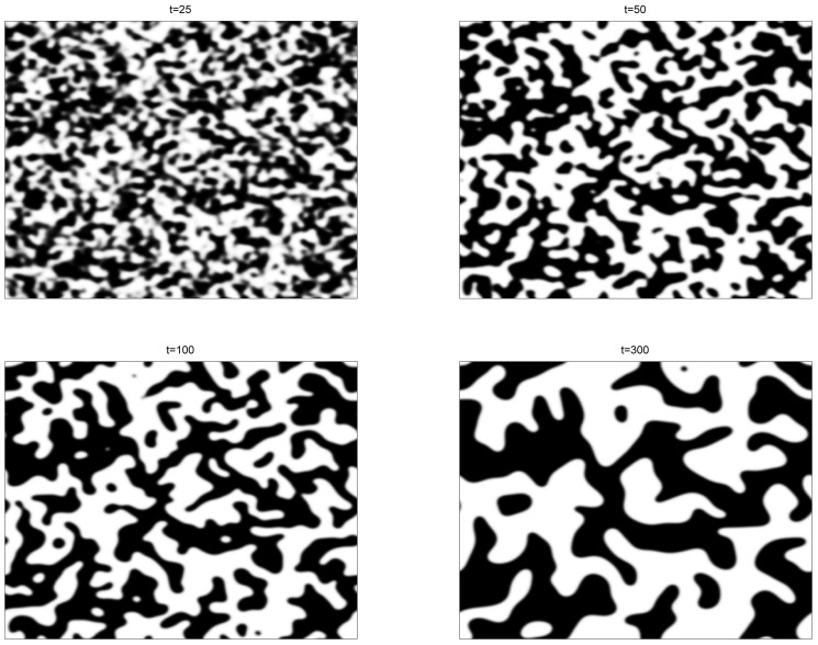
There are two characteristic length scales in this system, one is the system size (which is set to 1), the other is the local interaction radius r. So regarding the correlation length or the typical scale of opinion domains l, the dynamics can be divided into two stages: (1) l is smaller or comparable to r; (2) . In the second stage, the consensus is achieved when l grows up to 1. Figure 1 present snapshots of solution of the mean-field equation. They illustrate the formation of opinion domains and the coarsening of the spatial structure.

Figure 1. Snapshots of numerical solution of the mean-field equation as defined by Eq. (4).

Snapshots are taken at t = 25, 50, 100, 300, the scale of opinion domains are much bigger than r = 0.01. Black stands for opinion A, white stands for opinion B and gray stands for the coexistence of two types of opinions. The consensus is achieved at t ≈ 10⁴.

To study the spatial coarsening, we consider the pair correlation function C(L, t) defined by the conditional expectation of spin correlation.

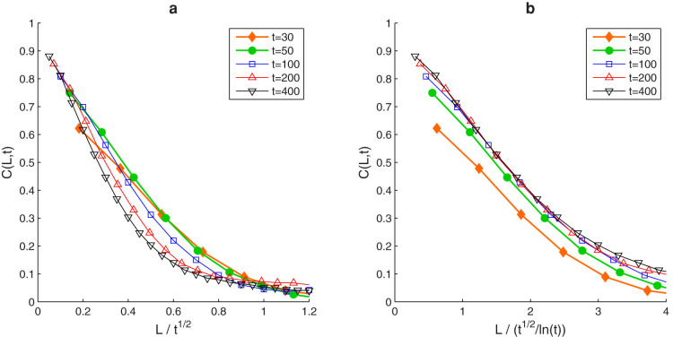
Figure 1 implies there exists a single characteristic length scale l(t) so that the pair correlation function has a scaling form , where the scaling function does not depend on time explicitly. For coarsening in most systems with non-conserved order parameter such as the opinion dynamics on a d-dimensional lattice, the characteristic length scale is ²³. According to the numerical results in Fig. 2, the length scale for opinion dynamics on RGG at the early stage (t = 30,50) is also , but at the late stage (t = 100,200,400), the length scale fits more precisely simulation results than the previous one.

Figure 2. Scaling function for the pair correlation function at times t = 30, 50, 100, 200, 400.

Overlapped curves indicate correct scaling of L. Simulations are done for the case N = 10⁵, r = 0.01, 〈k〉 = 31.4. L is normalized by the length scale (a) and (b) .

Stationary solution

Here, we find all the possible stationary solutions of the mean-field equation Eq. (4). Taking , we obtain

The eigenvalues of the linear dynamical system are both negative, so is stable. Applying the definition of s(x, y) and μ(x, y), we have

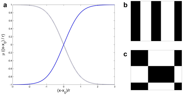
Once we solve the above integral equation, we can retrieve the stationary macrostate n*(x, y) by Eq. (7). Taking μ(x, y) as a constant, we find three solutions μ(x, y) = ±1 or 0. μ(x, y) = ±1 are both asymptotically stable, while μ(x, y) = 0 is unstable. Another class of solution is obtained by taking μ(x, y) = μ(x) (or similarly μ(x, y) = μ(y)). The solution consists of an even number of stripe-like opinion domains demarcated by two types of straight intermediate layers parallel to one side of the unit square D as shown in Fig. 3(b). With the boundary condition μ(−∞) = −1, μ(+∞) = 1 or vice versa, we solve the two types of intermediate layers as shown in Fig. 3 (a). The intermediate layers are of the scale r and can be placed at arbitrary x₀ ∈ [0, 1). This class of solution is neutrally stable. Finally, there is another class of solution shown in Fig. 3(c) with intermediate layers both in x and y directions and opinion domains assigned as a checker board. This type of solution is unstable at the intersections of two types of intermediate layers. The latter two classes of solutions can be easily generalized to the cases when the intermediate layers are not parallel to x or y axis. Later we will show that in stationary solutions all the curvature of the opinion domain boundary has to be 0, so the solutions mentioned above are the only possible stationary solutions.

Figure 3. Stationary solution.

(a) Two types of intermediate layers for stationary solution . x₀ is the location of the intermediate layer. The slope of the intermediate layer at x = x₀ is about γ*/r = 1.034/r. (b) Stripe-like stationary solution, neutrally stable. (c) Checker-board-like stationary solution, unstable.

In conclusion, considering the stability, the final state of the macrostate dynamics can be: (1) all A or all B consensus states which are both asymptotically stable, (2) stripe-like solution. The probability for the dynamics stuck in the stripe-like state before achieving full consensus is roughly in analogy to similar cases in continuum percolation and spin dynamics²⁹,³⁰.

Two-time-scale separation of mean-field equation and comparison with other models

One important observation regarding the macrostate dynamics is that the change of local mean field is usually much slower than the convergence of local macrostate to its local equilibrium . Let , , . The following equation shows the exponential rate of convergence of :

The largest eigenvalue is . So the typical time scale τ_n of the convergence of the local macrostate is which is independent of time and system size. The typical time scale τ_f of the change of the local mean field is inversely proportional to the propagation speed v of opinion domain boundaries, and as we will show later, is of the order where R is the curvature of the opinion domain boundary. Therefore, for both long time (R grows to infinity along with the time t) and big systems (in the sense that ).

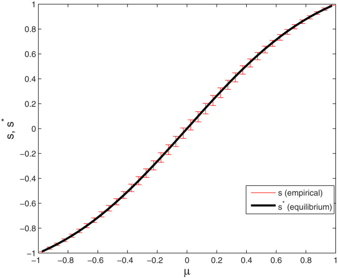
Fig. 4 shows the significant two-time-scale separation observed in numerical results. The equilibrium value of the local order parameter, s*, can be predicted by the local mean field, . In Fig. 4, we present the empirical local order parameter s for different local mean field values μ and show that it is very close to its local equilibrium s*.

Figure 4. Comparing the empirical local order parameter s from numerical simulation and the equilibrium s* for different local mean fields μ's.

The solid line stands for s*. The error bars present the means and standard deviations of s that is the empirical local order parameter for the given μ in numerical simulations.

Since , we have

This ODE is quite relevant to reaction-diffusion systems. On the right hand side, the coefficient is easy to get rid of by scaling the time τ = t/2. After the scaling, the first term is diffusive since (μ − s) is the continuum approximation of the Laplace operator on RGG network acting on s. The second term n_ABμ is the local reaction term. Though classified rigorously, it is non-local as defined in reaction-diffusion system, it represents a reaction in local neighborhood B_r(x, y). The adiabaticity of the dynamics implies that the diffusion is much slower than the local reaction. We can obtain an approximated ODE for slow time scale dynamics in a closed form by estimating n_AB by its local equilibrium .

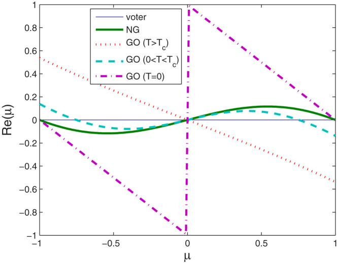
The qualitative behavior of the reaction-diffusion system is determined by the linear stability of the reaction term²⁴. In this sense, Eq. (12) provides clear differentiation between dynamics in our model and in the voter model, the majority game and the Glauber ordering. Taking a similar approach, we find that the voter model on RGG is purely diffusive, i.e. the reaction term is 0. For the Glauber ordering, the reaction term is tanh(βJμ) − μ in which β is the inverse of temperature and J is the interaction intensity. Fig. 5 shows the reaction term Re(μ) for the voter, NG, and Glauber ordering (GO) at different temperatures. The majority game, NG, and Glauber ordering at zero temperature have reaction terms with the same equilibria and stability (±1 stable, 0 unstable). Thus, the mean-field solutions of these models behave similarly. However, at the level of the discrete model, the NG on RGG will always go to a microstate corresponding to some stationary mean-field solution, while Glauber ordering at zero temperature on RGG may get stuck in one of many local minima of its Hamiltonian.

Figure 5. Reaction term Re(μ) for voter, NG and Glauber ordering (GO) at different temperatures.

Boundary evolution

The evolution of the opinion domains is governed by a very simple rule. The boundary of opinion domains propagate at the speed v that is proportional to its curvature 1/R, i.e. . Here, α is a constant defined by the average degree 〈k〉. In Methods, we provide a heuristic argument and using the perturbation method prove this relation for the mean-field equation, i.e. the case when 〈k〉 → ∞. This behavior is common for many reaction-diffusion systems and it is qualitatively the same as the behavior of Glauber ordering at zero temperature²³,³¹.

Following the rule of boundary evolution minimizes the length of the domain boundary. A direct consequence of this fact is that if any stationary solution exists, its boundaries must be all straight (geodesic), confirming our conclusion about the stationary solutions found in the previous paragraph. Since global topology is irrelevant to our derivation, this relation applies also to other two-dimensional manifolds. The manifold considered here is the torus embedded in 2D Euclidean space. However, for the standard torus embedded in 3D Euclidean space, the topology is the same but metrics are not, hence the geodesics are different. Therefore, there are quite different and more complicated stationary solutions there. Another example is the sphere in 3D space. On the sphere, the only inhomogeneous stationary solution consists of two hemispherical opinion domains, because the great circle is the only closed geodesic on a sphere.

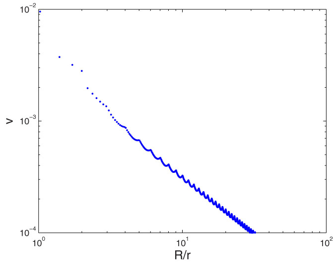
The numerical result presented in Fig. 6 confirms this relation. In Fig. 6, we gather 10⁶ data points from numerical solutions of the macrostate equation, using different initial conditions, taking snapshots at different times, tracking different points on the boundary and calculating the local curvature radius R and boundary propagation speed v. These data points in the double-log plot are aligned well with the straight line with slope −1. The curve formed by data points is jiggling with some period because we implemented the numerical method on a square lattice, so the numerical propagation speed is slightly anisotropic.

Figure 6. Propagation speed v of the boundary of opinion domains vs. curvature radius R. Data points are gathered from 100 runs of macrostate equation with different initial conditions.

In each run, propagation speed and curvature radius are calculated for 10000 points on the boundary.

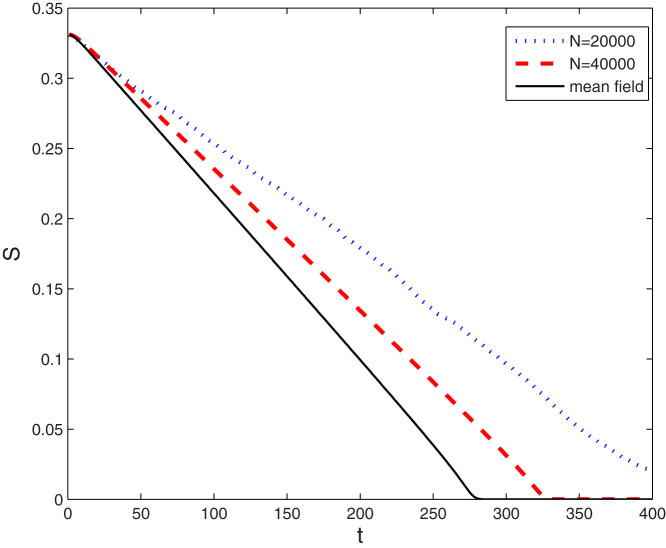
Another way to confirm this rule is to consider a round opinion domain with initial radius R₀. Given , the size of this opinion domain decreases as when . This relation is shown in Fig. 7. In simulations, the size of opinion domain S(t) is evaluated by where N_A,N_AB are the total numbers of A, AB nodes, respectively. We also observe from this plot that α increases with average degree 〈k〉 and converges to its upper bound when 〈k〉 → ∞.

Figure 7. The size of an opinion domain S as a function of time with r = 0.05.

The initial radius of the opinion domain is R₀ = 0.325. The straight line is for the numerical solution of mean-field equation. The dotted line and dash line are for simulation of discrete model with N = 10000 and 〈k〉 = 78.5, as well as with N = 20000 and 〈k〉 = 157), respectively.

Impact of committed agents

We now consider influencing the consensus by committed agents. In sociological interpretation, a committed agent is one who keeps its opinion unchanged forever regardless of its interactions with other agents. The effect of committed agents in the NG has been studied in¹⁵,¹³,²². A critical fraction of committed agent is found for NG-LO on complete graph which is also relevant here. In our setting, a fraction q of agents are committed to opinion A, and all other agents are uncommitted and hold opinion B. The macrostate with committed agents is still defined by Eq. (4), but the definition of local mean field μ is replaced by

Generally, q can vary on the x-y plane, but we only consider the case that q is a constant, i.e. the committed agents are uniformly distributed. Then we reanalyze the stationary solution. Firstly there is a critical committed fraction q_c which is exactly the same as that on complete graph. When q > q_c, the only stationary solution is μ(x, y) = 1 and it is stable. When q < q_c, there are three solutions, of which two μ(x, y) = 1, are stable, and the third is unstable. Besides there is a class of stationary solutions when the committed fraction is below the critical. They are analogues of the stripe-like solutions in the non-committed agent case. The evolution of the boundary can be interpreted as a mean curvature flow. In such view, the fraction of agents committed to A opinion exert a constant pressure on the boundary surface from the side of A opinion domain. Similarly, agents holding opinion B exert a pressure from the side of B opinion domain. So the stationary solution will contain opinion domains in the form of disks with critical radius R_c for which the pressure arising from the curvature offsets the pressure from the committed fraction; thus we have . This type of stationary solutions are unstable, the round disk of the opinion domain will grow when R > R_c and will shrink when R < R_c. In the first case, when the typical length scale of opinion domains grows beyond 2R_c, the system will achieve consensus very quickly.

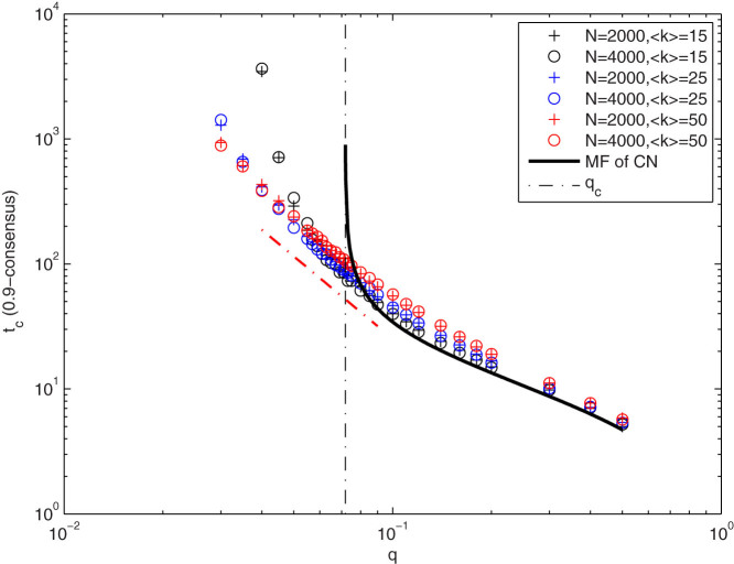
On the basis of the above stability analysis, we then analyze the dependence of the consensus time on the system size N, the committed fraction q, and the average degree 〈k〉, and show our conclusions are consistent with the numerical results in Fig. 8 which for a given fraction α (α = 0.9 in the figure) depicts the time for α-consensus in which at least fraction α of agents hold the same opinion. The time to achieve α–consensus is independent of N both according to the mean field prediction and numerical plots. When q > q_c the dynamics will converge to its unique local equilibrium μ = 1 at all locations simultaneously. The consensus in this case is close to that on the complete network, especially when 〈k〉 tends to infinity. In the opposite case, when q < q_c, the process to consensus is twofold - before and after the A opinion domain achieves the critical size 2R_c. After this criticality, the process is just the extension of the opinion domain driven by the mean field Eq. (4). This stage is relatively fast and the consensus time is dominated by the duration of the other stage, the one before the criticality, in which the dynamic behavior is a joint effect of the mean field and the random fluctuation we neglect in mean field analysis. Assuming the dynamics was purely driven by the random fluctuation, the typical length scale of opinion domains would have the scaling at the early stage, hence the time scale of this stage would be , i.e. O(q⁻²). If the dynamics was purely driven by the mean field, the A opinion domain would never achieve the critical size. The actual dynamics behavior is in between the two extreme cases. When 〈k〉 decreases, the fluctuation level relative to the mean field becomes higher, leading to faster consensus. In Fig. 8, linear regression for the data points 0.6 < q < q_c gives t_c ~ q^−γ in which γ = 2.59, 2.34, 2.19 for <k > = 50, 25, 15 respectively, where γ = 2 is the value corresponding to the purely random extreme case.

Figure 8. Time t_c for 0.9-consensus for NG on RGG with different fractions (q) of committed agents with direct simulation on networks with average degrees 〈k〉 = 15, 25, 50, and network sizes N = 2000, 4000.

The solid black curve shows the mean field prediction of NG on the complete network(CN) as the limit case when 〈k〉 → ∞. The slope of the red data points near q_c is −2.19.

Two observations here may have meaningful sociological interpretation:

1. When 〈k〉 → ∞, for both q < q_c and q > q_c, the dynamics behavior converges to that on the complete networks, though the RGG itself may be far from the complete network (with r kept constant, the diameter of the RGG network is much larger than 1).

2. When q < q_c, committed agents are more powerful in changing the prevailing social opinion on RGGs with low average degree. It is similar to the result of the previous study²² on the social dynamics on sparse random networks but the “more powerful” is in a different sense meaning not the smaller tipping fraction (with longer consensus time), but the shorter time to consensus.

Discussion

On RGGs, the average degree of an agent 〈k〉 = πr²N is an important structural parameter which also strongly impacts the local dynamic behavior. There are two critical values of 〈k〉: One is for the emergence of the giant component, k_c1 = 4.512³²; The other one, k_c2, only applicable for finite-size networks, is for the emergence of the giant component with all vertices belonging to it. In this paper, we only considered the case when 〈k〉 is above the critical value k_c2 ~ ln N so that the network is connected²⁶.

We mainly focused on analyzing the mean-field equation of the NG dynamics on RGG. We predicted a number of behaviors, including the existence of metastable states, the two-time-scale separation, and the dependence of the boundary propagation speed on the boundary curvature. We demonstrated in detail that the evolution of the spatial domains for the two-word LO-NG is governed by coarsening dynamics, similar to the broader family of generalized voter-like models with intermediate states¹⁷,²⁰,²⁴,²⁵. However, there are still some behaviors that cannot be explained by the mean-field equation, such as: (i) in the large t limit, the scaling of correlation length is not as on the 2-d regular lattice, but ; (ii) the propagation speed increases along with the average degree 〈k〉 and its upper-bound is the mean field prediction, i.e., the 〈k〉 → ∞ case. So the major limitation of the mean-field equation derived from the geographic coarsening approach is that it neglects the fluctuation among replicas (see Methods) and loses the information about 〈k〉. The dependence of the dynamics on 〈k〉 is left for further study.

Methods

Geographic coarsening approach

First, we provide the equation for the evolution of microstate . Denote the probabilities for s_i taking values 1, 0, −1 as p_iA, p_iAB and p_iB, respectively. The master equation for spin s_i is given by

where is the probability for the i^th agent receiving a signal A, while μ_i is the local mean field defined as the average of the neighboring spins,

where (x_i, y_i) is the coordinate of the i^th agent and k_i is the degree of the i^th agent. Master equations for all spins together describe the evolution of microstate.

The motivation for geographic coarsening comes from the fact that RGG is embedded in a geographic space, so we may skip the level of agents and relate the opinion states directly to the geographic coordinates. Instead of taking into account the opinion of every agent, in geographic coarsening, we consider the concentration of agents with different opinions at a specific location. , s(x, y), f(x, y) are continuously differentiable w.r.t. x, y and t. We derive the equation of from Eq. (14) by taking limits,

The limit is done as follows

The coarsening based on the above limit is valid under either of the following two assumptions. The first is when the RGG is very dense (N → ∞) and keeps constant. The second is when we consider K replicas of RGG with the same set of parameters, and the summation above is over all replicas. In addition, keeps constant. Our derivation is actually based on the second assumption. However under the first assumption, the fluctuation is vanishing, and the dynamics behavior of a single run converges to the mean field result.

Propagation speed of the domain boundary

We show here the qualitative property of the boundary evolution by a heuristic argument. We consider a solution with the form where and with boundary conditions g(0) = −1 and g(∞) = 1. has an intermediate layer at R as shown in Fig. 3(a), so near R, . When , using moving coordinate where is unit wave vector, is spatial coordinate and v is the wave speed, Eq. (11) becomes

Here, μ can be approximated by

Then we make perturbation on Eq. (18) , , and so on, requiring s*(ξ = 0) = μ*(ξ = 0) = v* = s(ξ = 0) = 0, and obtain the equation for O(ξ)

At ξ = 0, , , and is γ*/r, the above equation becomes , so

Author Contributions

Z.W., C.L., G.K. and B.K.S. designed the research; Z.W. implemented and performed numerical experiments and simulations; Z.W., C.L., G.K. and B.K.S. analyzed data and discussed results; Z.W., C.L., G.K. and B.K.S. wrote and reviewed the manuscript.

Supplementary Material

Supplementary Information

Communications of Listener-Only 2-Word Naming Game

References

- Galam S. Sociophysics: A Review of Galam Models. Int. J. Mod. Phys. C 19, 409–440 (2008). [Google Scholar]
- Durlauf S. N. How can statistical mechanics contribute to social science? Proc. Natl. Acad. Sci. USA 96, 10582–10584 (1999). [DOI] [PMC free article] [PubMed] [Google Scholar]
- Castellano C., Fortunato S. & Loreto V. Statistical physics of social dynamics. Rev. Mod. Phys. 81, 591–646 (2009). [Google Scholar]
- Liggett T. M. Interacting Particle Systems (Springer-Verlag, New York, 1985). [Google Scholar]
- Castellano C., Vittorio L., Barrat A., Cecconi F. & Parisi D. Comparison of voter and Glauber ordering dynamics on networks. Phys. Rev. E 71, 066107 (2005). [DOI] [PubMed] [Google Scholar]
- Baronchelli A., Felici M., Caglioti E., Loreto V. & Steels L. Sharp transition towards shared vocabularies in multi-agent systems. J. Stat. Mech.: Theory Exp. P06014 (2006). [Google Scholar]
- Dall'Asta L., Baronchelli A., Barrat A. & Loreto V. Nonequilibrium dynamics of language games on complex networks. Phys. Rev. E 74, 036105 (2006). [DOI] [PubMed] [Google Scholar]
- Galam S. Application of statistical physics to politics. Physica A 274, 132–139 (1999). [DOI] [PubMed] [Google Scholar]
- Krapivsky P. L. & Redner S. Dynamics of Majority Rule in Two-State Interacting Spin Systems. Phys. Rev. Lett. 90, 238701 (2003). [DOI] [PubMed] [Google Scholar]
- Steels L. The synthetic modeling of language origins. Evolution of Communication 1, 1–34 (1997). [Google Scholar]
- Kirby S. Natural Language From Artificial Life. Artificial Life 8, 185–215 (2002). [DOI] [PubMed] [Google Scholar]
- Castelló X., Baronchelli A. & Loreto V. Consensus and ordering in language dynamics. Eur. Phys. J. B 71, 557–564 (2009). [Google Scholar]
- Xie J. et al. Social consensus through the influence of committed minorities. Phys. Rev. E 84, 011130 (2011). [DOI] [PubMed] [Google Scholar]
- Xie J. et al. Evolution of Opinions on Social Networks in the Presence of Competing Committed Groups. PLoS One 7, e33215 (2012). [DOI] [PMC free article] [PubMed] [Google Scholar]
- Zhang W. et al. Social Influencing and Associated Random Walk Models: Asymptotic Consensus Times on the Complete Graph. Chaos 21, 025115 (2011). [DOI] [PubMed] [Google Scholar]
- Baronchelli A. Role of feedback and broadcasting in the naming game. Phys. Rev. E 83, 046103 (2011). [DOI] [PubMed] [Google Scholar]
- Baronchelli A., Dall'Asta L., Barrat A. & Loreto V. Topology-induced coarsening in language games. Phys. Rev. E 73, 015102(R) (2006). [DOI] [PubMed] [Google Scholar]
- Dall'Asta L., Baronchelli A., Barrat A. & Loreto V. Agreement dynamics on small-world networks. Europhys. Lett. 73, 969–975 (2006). [Google Scholar]
- Lu Q., Korniss G. & Szymanski B. K. The Naming Game in social networks: community formation and consensus engineering. J. Econ. Interact. Coord. 4, 221–235 (2009). [Google Scholar]
- Lu Q., Korniss G. & Szymanski B. K. Naming games in two-dimensional and small-world-connected random geometric networks. Phys. Rev. E. 77, 016111 (2008). [DOI] [PubMed] [Google Scholar]
- Lu Q., Korniss G. & Szymanski B. K. Naming Games in Spatially-Embedded Random Networks. in Proceedings of the 2006 American Association for Artificial Intelligence Fall Symposium Series, Interaction and Emergent Phenomena in Societies of Agents (AAAI Press, Menlo Park, CA 2006), pp. 148–155; arXiv:cs/0604075v3. [Google Scholar]
- Zhang W., Lim C. & Szymanski B. K. Analytic treatment of tipping points for social consensus in large random networks. Phys. Rev. E 86, 061134 (2012). [DOI] [PubMed] [Google Scholar]
- Bray A. J. Theory of Phase Ordering Kinetics. Adv. Phys. 51, 481–587 (2002). [Google Scholar]
- Vazquez F. & Lopez C. Systems with two symmetric absorbing states: Relating the microscopic dynamics with the macroscopic behavior. Phys. Rev. E 78, 061127 (2008). [DOI] [PubMed] [Google Scholar]
- Dall'Asta L. & Galla T. Algebraic coarsening in voter models with intermediate states. J. Phys. A: Math. Theor. 41, 435003 (2008). [Google Scholar]
- Penrose M. Random geometric graphs (Oxford University Press, 2003). [Google Scholar]
- Collier T. C. & Taylor C. E. Self-organization in sensor networks. J. Parallel. Distr. Com. 64, 866–873 (2004). [Google Scholar]
- Cox J. T. Coalescing random walks and voter model concensus time on the torus in Zd. Ann. Probab. 17, 1333–1366 (1989). [Google Scholar]
- Spirin V., Krapivsky P. L. & Redner S. Freezing in Ising ferromagnets. Phys. Rev. E 65, 016119 (2001). [DOI] [PubMed] [Google Scholar]
- Barros K., Krapivsky P. L. & Redner S. Freezing into stripe states in two-dimensional ferromagnets and crossing probabilities in critical percolation. Phys. Rev. E 80, 040101(R) (2009). [DOI] [PubMed] [Google Scholar]
- Osher S. Fronts propagating with curvature-dependent speed: algorithms based on Hamilton-Jacobi formulations. J. Comput. Phys. 79, 12–49 (1988). [Google Scholar]
- Dall J. & Christensen M. Random geometric graphs. Phys. Rev. E 66, 016121 (2002). [DOI] [PubMed] [Google Scholar]
Associated Data
This section collects any data citations, data availability statements, or supplementary materials included in this article.
Supplementary Materials