

Abstract
A computational model utilizing grid and finite difference methods was developed to simulate focused ultrasound functional neurosurgery interventions. The model couples the propagation of ultrasound in fluids (soft tissues) and solids (skull) with acoustic and visco-elastic wave equations.
The computational model was applied to simulate clinical focused ultrasound functional neurosurgery treatments performed in patients suffering from therapy resistant chronic neuropathic pain. Datasets of five patients were used to derive the treatment geometry. Eight sonications performed in the treatments were then simulated with the developed model.
Computations were performed by driving the simulated phased array ultrasound transducer with the acoustic parameters used in the treatments. Resulting focal temperatures and size of the thermal foci were compared quantitatively, in addition to qualitative inspection of the simulated pressure and temperature fields.
This study found that the computational model and the simulation parameters predicted an average of 24 ± 13 % lower focal temperature elevations than observed in the treatments. The size of the simulated thermal focus was found to be 40 ± 13 % smaller in the anterior–posterior direction and 22 ± 14% smaller in the inferior–superior direction than in the treatments. The location of the simulated thermal focus was off from the prescribed target by 0.3 ± 0.1 mm, while the peak focal temperature elevation observed in the measurements was off by 1.6 ± 0.6 mm.
Although the results of the simulations suggest that there could be some inaccuracies in either the tissue parameters used, or in the simulation methods, the simulations were able to predict the focal spot locations and temperature elevations adequately for initial treatment planning performed to assess, for example, the feasibility of sonication. The accuracy of the simulations could be improved if more precise ultrasound tissue properties (especially of the skull bone) could be obtained.
1. Introduction
Transcranial focused ultrasound is an emerging modality for treatment of brain disorders. Phase I clinical trials have included studies such as thermal ablation of brain tumors [28] and treatment of chronic neuropathic pain [23, 27]. There are also ongoing clinical trials for the treatment of essential tremor in a number of clinical trial centers [25, 18]. Potential future applications of focused ultrasound neurosurgery include targeted drug delivery [19] and thrombolysis [30] to name a few.
Applying transcranial focused ultrasound is not without issues. These issues include phase aberrations caused by the skull [42, 38], potential standing waves [3] and undesired tissue heating outside the focal region [36].
To compensate the phase aberration caused by the skull, fast numerical methods have been developed to compute approximative phase corrections for the phased array [6]. Although computationally heavier, in addition to approximative methods of estimating the phase aberrations, full-wave phase inversion can be applied to increase accuracy [1, 12, 36, 37, 26]. By taking the shear waves into account the focusing, i.e. the constructive interference of the individual acoustic fields in the target volume, can be further enhanced [9], especially near the skull surface [33]. In addition to computational methods to correct for the aberrations, other methods of focusing have also been devised, based on motion-sensitive MR imaging [24], droplet vaporization [21], acoustically induced cavitation signal [20], micro-receivers [5], and time-reversal mirrors [32]. However, none of these methods are at a state to be clinically implemented.
Standing waves are caused by sound waves propagating in opposite directions with similar amplitudes. In transcranial ultrasound this situation can occur mainly in three regions: between the transducer and the skull, within the calvaria, and within the brain. Reflections between the transducer and the outer skull could affect the operation of the transducer as part of the reflecting sound affects the vibration of the transducer. Standing waves within the calvaria itself can create localized heat sources as demonstrated in [12]. Localized standing-wave patterns can also be created within the brain in situations where a small transducer is sonicating through the skull: when the ultrasound beam reflects from the inner skull surface within the brain it could reflect in such a way that the beam interferes with the incident beam, creating a standing-wave pattern [3]. To reduce the standing-wave effects, randomized phase modulation [39], frequency sweeping [40] and periodic linear chirp methods have been developed [15]. By using a low f -number transducer, the standing-wave phenomenon is also reduced, due to highly localized pressure fields [37].
High ultrasound absorption in the skull causes heating as the ultrasound beam passes through the calvaria and into the brain. The increase in temperature could diffuse into the brain tissue, causing undesired heating. The issue can be circumvented by using active cooling of the skull [22] and large-area transducers maximizing the surface area of the skull to transmit the ultrasound through [8]. In addition to heating the calvaria, the ultrasound beam will hit the skull base after passing through the focus. This could also lead to undesired heating and potential damage if the sonication targets are close to the skull base [36]. Furthermore, ultrasound beams reflecting back and forth within the brain could, in principle, be interacting in such a way that the beams would create an unintended secondary focus in the brain. Such a situation has not been found in an extensive study using 3D MR-thermometry and skull phantoms with a low-frequency therapeutic device [29].
Motives for this manuscript include verifying whether a clinical treatment can be accurately simulated using a computational model. Computational models are important for non-invasive treatment planning and device design, as well as for in situ control. Accurate models also allow for parametric studies to optimize treatment protocols without going through often difficult or time-consuming experiments.
2. Materials and methods
2.1. Patients
Treatment data from five patients (denoted A–E) obtained during a clinical trial of the treatment of chronic neuropathic pain reported in [27, 23] were used for this study. The clinical trial was approved by Ethics Commission of the State of Zurich, Subcommission Psychiatry, Neurology, Neurosurgery, (registration No. E-04/2008, approval date 19.05.2008); and Swissmedic (registration No. 2008-MD-0010, approval date 24.07.2008). The anatomical data of the patients and sonication parameters applied in the treatments were used as inputs in the simulation model, and the simulated temperature distributions were then compared with temperature maps obtained intraoperatively using MR-thermometry.
2.2. Therapy device
The therapy device (ExAblate 4000, InSightec, Israel) used in this study is composed of MR-compatible phased array, amplifier, and driving electronics and the controlling work station. The phased array has 1011 transducers laid in hemispherical configuration with 30 cm aperture and 15 cm radius of curvature. The phased array is operated at 650 kHz. The therapy device is integrated into a clinical high-field MR-scanner (Signa HDx 3T MRI, GE Healthcare, USA).
2.3. Imaging methods
The resolution of the CT-scans (Brilliance 40, Philips Healthcare, Netherlands) used for the phase calculation by the therapy device were 1 mm × 0.49 mm × 0.49 mm. The CT scans were taken prior to the treatment using bone reconstruction kernel.
In the beginning of the treatment, fast spin-echo T2-weighted MR images of the patients’ heads were acquired for transducer and CT registration. Stereotactic navigation for targeting the sonications was done using T2-weighted and 3D T1-weighted inversion recovery MR images. During the sonications, a fast spoiled gradient echo sequence was used to map the temperature elevation. Parameters used in the MR-imaging sequences are shown in Table 1.
Table 1.
MR-imaging parameters used in this study for registration, navigation and thermometry.
| T2W | 3DT1IR | Thermometry | |
|---|---|---|---|
| TR (ms) | 2880 | 29.0 | 39.3 |
| TE (ms) | 102 | 10.5 | 19.5 |
| TI (ms) | 500 | ||
| Flip angle (°) | 20 | 30 | |
| Slice thickness (mm) | 2 | 2 | 3 |
| Bandwidth (kHz) | 15.63 | 27.78 | 5.68 |
| FOV (cm) | 24 | 26 | 28 |
| Matrix size | 384 × 256 | 512 × 358 | 256 × 128 |
2.4. Sonications
Phasing of the sonications was computed using the control software of the therapy device. Before sonications the system computes the phase aberration caused by the skull. At the same time, it also estimates the transmitted sound-field amplitude and computes sonication amplitudes for each phased array element individually to achieve optimal sonication. The phase aberration is estimated based on such factors as the incident and transmitted angle through the skull for each transducer element as well as the skull thickness and density at point of transmission [6]. The system also automatically disables phased array elements that would not be contributing to focal pressure amplitude due to, for example, too large angle of incidence at the skull surface.
Either axial, sagittal or coronal MRI-thermometry scans were performed during the sonications, based on the decision of the neurosurgeon. The decision was made based on ad hoc risk analysis that aims at protecting critical structures around the prescribed target, by choosing the scanning plane accordingly. The target volumes of patient A, as well as the relative orientation of the patient and the transducer, are shown in Figure 1. Similar target locations and transducer patient orientation were used for patients B through E.
Figure 1.
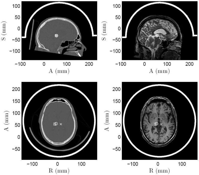
Sagittal (top) and axial (bottom) slices of the unsegmented CT scans showing the skull geometry (left column) and MR scans used for stereotactic navigation in patient A (right column, top: T2-weighted spin-echo, bottom: T1-weighted inversion recovery). White lines denote the transducer orientation. Target volumes 1–4 are marked with cross, circle, square, and plus sign respectively.
During the treatments, patients received 14 to 24 continuous wave (full duty-cycle) sonications, with sonication durations ranging from 5 to 20 s and prescribed average sonication power between 5 and 1500 W. The location of the acoustic focus was determined by low power sonications and then the sonications were repeated with increasing power until desired temperature elevation was reached. A cooling time of roughly one minute per every 1 kJ of sonicated energy followed each sonication, to allow the elevated temperature in the patient to dissipate. The number of active elements varied between 840 and 957. All stereotactic targets were located in the posterior part of the centro-later nucleus of the thalamus (CLp). Patients A and C received bilateral treatments, while patients B, D and E received unilateral treatment. Four sonications in patient A were chosen for analysis; whereas in patients B through E, one high power sonication for each was chosen. The sonications were chosen based on ad hoc analysis of the measured temperature fields, and the sonications with the clearest spatial and temporal focus were chosen for the analysis. The sonication parameters of the analysed sonications are shown in Table 2. Before some of the investigated sonications, prior treatment sonications had been performed. The number of prior sonications and their total sonicated energy are shown in Table 3. The measured temperature maps of the sonications for patient A are shown in Figure 2. The figure shows the last MR thermometry phase image before the end of the sonications. Similar temperature fields were observed in patients B through E. Due to the imaging parameters, the MR thermometry scans are not at the exact moment when the sonication ends.
Table 2.
Parameters of the simulated sonications 1–4 in patient A, and the sonications in patients B–E: sonication duration, sonication power, and number of active elements in the sonication.
| Patient | Sonication number | Duration (s) | Power (W) | Elements |
|---|---|---|---|---|
| A | 1 | 15 | 950 | 941 |
| 2 | 15 | 500 | 941 | |
| 3 | 20 | 800 | 957 | |
| 4 | 20 | 850 | 954 | |
| B | 10 | 820 | 941 | |
| C | 15 | 1000 | 840 | |
| D | 12 | 1500 | 943 | |
| E | 15 | 650 | 878 |
Table 3.
The sonications delivered to the patients before the investigated sonications. Shown are the number of sonications and the total sonicated enery.
| Patient | Sonication number | Prior sonications | Prior energy (kJ) |
|---|---|---|---|
| Aa | 1 | 9 | 45.80 |
| 2 | 0 | 0.00 | |
| 3 | 4 | 41.25 | |
| 4 | 2 | 23.50 | |
| Bb | 13 | 77.90 | |
| C | 8 | 50.00 | |
| Dc | 17 | 133.10 | |
| E | 14 | 51.50 |
Sonication 1 is on contralateral side of sonications 2, 3 and 4. Sonications 2 and 3 are separated by 5.5 mm, 3 and 4 by 1 mm and 2 and 4 by 5.0 mm.
Values include prior sonications delivered 2.6 mm from investigated sonication.
Values include prior sonications delivered 0.5 mm from investigated sonication.
Figure 2.
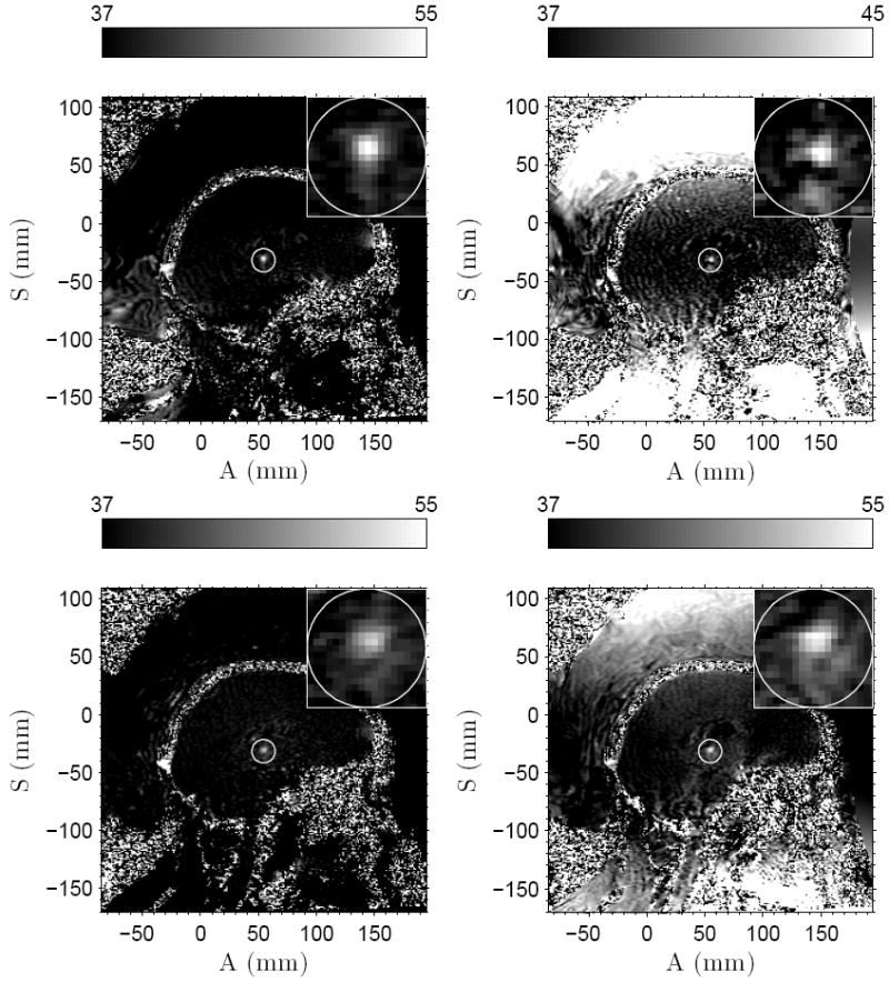
Measured temperature fields at the end of sonications for patient A for sonications 1–4, counting from left to right and top to bottom. The time instances of the temperature fields are 11.9, 11.9, 11.9, and 18.6 s respectively. The prescribed focus position is circled and a close-up is shown in the small insert for 1cm×1cm region.
2.5. Simulation models
Ultrasound propagation in fluids and soft tissues can be described with the acoustic wave equation of fluids [35] for pressure p
| (1) |
where c is the sound speed, ρ is the density and α is the attenuation coefficient. Shorthand notation for the first and second order temporal derivatives is used. Propagation of ultrasound in the skull on the other hand is described by the visco elastic wave equation of solids written in terms of particle displacement u as [2]
| (2) |
where λ and μ are the first and second Lamé coefficients and η and ξ are the first and second viscosity parameters.
Equations (1) and (2) are coupled on the skull-tissue interfaces by imposing continuous particle displacement and force in the surface normal direction and vanishing of the force component in tangential plane.
The equations were solved using a hybrid model composed of finite difference time domain [14] and the so-called grid method [44]. Details of the simulation model are given in the appendix.
Simulation geometry was derived from the data files exported by the therapy device. The data files contain CT scan of the skull, positions of the phased array elements, and 3D transformation matrices needed to align them. As the accurate shape of the phased array elements was not known, they were presumed to be piston transducers with maximum possible radius without overlap. CT scans were segmented by thresholding, and the bone density was estimated based on the CT intensity [10]. Spatial discretization of Δh = 231 μm and temporal discretization of Δt = 11 ns were used. These correspond to 10 points per wavelength in water with sound speed of 1500 m/s and 147 points per cycle at the driving frequency of 650 kHz. Maximum Courant-Friedrichs-Lewy number (γ = cΔtΔh−1 with c being either the sound speed in the fluid or longitudinal or shear sound speed in the solid) was 0.15. The sonications were simulated for 334 μs, allowing the sound to travel for about 50 cm in water. This was done to ensure that a stable acoustic field pattern was reached.
The number of spatial discretization points in the simulation domain varied between 1311 × 1337 × 1028 and 1338 × 1363 × 1120 points while the number of temporal points was 31899. The phased array transducer elements were driven with a sinusoidal signal that started from zero amplitude and increased linearly to the prescribed sonication amplitude in five cycles. The sound was brought to the simulation domain using Neumann boundary condition on the phased arrays surface. Absorbing boundary condition was used on other boundaries.
At the end of the simulations, for each point in the simulation domain, discrete temporal Fourier transformation was computed for the last two cycles of sonication. This was done to obtain an estimate of the stable pressure amplitude and phase distribution within the simulation domain. Time-varying pressure at the focus was collected during the simulations. The simulation geometry differed from the treatments such that, in the simulations, the head was presumed to be immersed completely in fluid. This might have some impact on the results. The material parameters used for the water and the soft tissue are shown in Table 4.
Table 4.
Thermal and acoustical parameters of water and soft tissue as used in the simulations. The parameters shown are based on the values presented in [17, 13, 11, 12].
| Material | ρ (kg/m3) | c (m/s) | α (Np/m) |
|---|---|---|---|
| Water | 1000 | 1500 | 0 |
| Soft tissue | 1030 | 1562 | 4.3 |
|
| |||
| Material | κ (W/°Cm) | C (J/kg°C) | W (1/s) |
|
| |||
| Soft tissue | 0.528 | 3640 | 8.33 · 10−3 |
|
| |||
| Material | ρb (kg/m3) | Cb (J/kg°C) | Tb (°C) |
|
| |||
| Blood | 1030 | 3620 | 37 |
The longitudinal sound speed cL and attenuation αL of the skull were interpolated based on [34]. For shear sound speed and attenuation, the values of and were used, because no experimental data were found for these parameters as a function of density. The scaling factors for the shear sound speed and attenuation are based on values presented in [43]. Material parameters used for the skull are shown in Figure 3.
Figure 3.
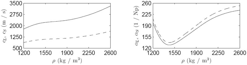
Material parameters used for the skull. Longitudinal (——) and shear (- - - -) sound speeds cL and cS on the left and corresponding attenuations αL and αS on the right as a function of the skull-density ρ [34].
The bio-heat equation [31] was used to simulate the temperature field T in the vicinity of the focus
| (3) |
where ρ is the density, C is the specific heat capacity, κ is the thermal conductivity, ρb, Cb, W and Tb are the density, the specific heat capacity, the perfusion rate and the temperature of the blood and Q is the absorbed power density. For the fluids Q can be computed as
| (4) |
where |p| is the pressure amplitude.
Equation (3) was solved using a semi-analytical approach [16]. Performing spatial Fourier transformation for the equation with constant material parameters reduces it into linear ordinary differential equation. After solving the ordinary differential equation for all spatial frequencies, an inverse Fourier transformation returns the temperature distribution.
Thermal simulations were computed in a smaller grid of 101 × 101 × 101 points, spanning a volume of 23 mm × 23 mm × 23 mm, with the same discretization as the acoustical simulations. The simulation volume was centered at the acoustic focus and was sufficiently large to allow for accurate focal temperature simulations. In order to make thermal simulations physically comparable with the MR measurements, the simulated temperature fields were spatially averaged over the size of the MR voxels of 1 mm × 1 mm × 3 mm. Thermal parameters used in the simulations are shown in Table 4.
In the simulated sonications the phase and amplitude of the phased array elements were the same as used during the treatments. In addition to treatment simulations, simulations were performed with the geometry of patient A and sonication one to see the effects of uncertainties in the phase correction, blood perfusion, modeling the skull as either fluid or solid, and the attenuation and the sound speed of the skull have on the focal temperatures.
The simulations were computed on HP CP4000 BL ProLiant cluster vuori (Finnish IT Center for Science (CSC)). Eight computing nodes, each having two six-core 2.6 GHz AMD Opteron 64-bit processors, were used for each simulation. The computing nodes communicated through InfiniBand network. The computation time for a single simulation was on average 65 ± 3 h for sonications with the skull modeled as solid, while the total memory use of the simulation model was around 64 GB. The simulation time when using the simplified model, where the skull is modeled as a fluid, was 40 h.
3. Results
Figure 4 shows the simulated pressure amplitude distributions for sonication four in patient A, with respect to the focal pressure amplitude. Three perpendicular slices are centered at the focus with dashed lines demarking the prescribed target. Clear focus at the desired location is achieved. Table 5 shows the simulated focal pressure amplitudes for the treatment sonications.
Figure 4.
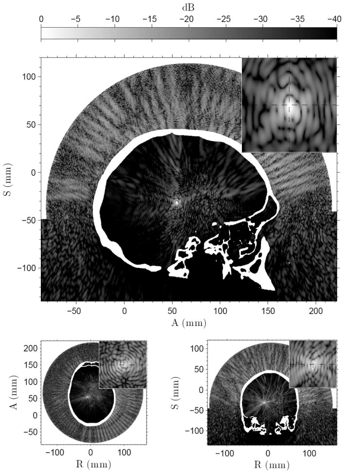
The simulated pressure amplitudes for sonication four in patient A. The small insert in the top right corner of the figures shows 1 cm × 1 cm closeup around the prescribed target, marked by the cross-section of the dashed lines. Pressure field shown for the sagittal (top), axial (bottom left), and coronal (bottom right) slices.
Table 5.
Measured and simulated temperatures at the end of the sonication for each patient. Sonication index for patient A in parentheses. For the measurements, thermal data from a 3 × 3 voxel neighbourhood centered at the focus is shown: average temperature at the end of the sonication with standard deviation, and in parentheses minimum and maximum temperature. For the simulations, the peak focal temperature after MR-voxel averaging is shown, as well as the focal pressure amplitude.
| Patient | Measured (°C) | Simulated (°C) | Focal pressure (MPa) |
|---|---|---|---|
| A (1) | 53.1 ± 2.4 (48.8/56.3) | 51.5 | 3.87 |
| A (2) | 45.2 ± 1.3 (43.3/47.2) | 44.2 | 2.65 |
| A (3) | 53.0 ± 1.7 (50.8/55.7) | 46.3 | 2.75 |
| A (4) | 51.4 ± 3.4 (44.6/54.9) | 47.5 | 2.94 |
| B | 54.1 ± 2.5 (50.5/57.8) | 48.6 | 3.60 |
| C | 56.8 ± 2.5 (53.7/60.9) | 51.2 | 3.45 |
| D | 60.5 ± 1.6 (58.4/62.8) | 58.8 | 5.24 |
| E | 52.7 ± 2.5 (49.0/57.2) | 47.3 | 3.16 |
Figure 5 shows close-ups of the measured thermal foci 1–4 in patient A and the corresponding simulated temperature fields. The temperatures shown are spatially averaged over the size of the MR thermometry voxels. This is performed to take into account the partial volume effects caused by the MR imaging. The figure also shows the simulated and measured temperatures as a function of time at the peak temperature elevation of the simulation and measurement respectively. The simulations resulted in similar temperatures as in the measurements, apart from sonication three. However, the simulated post-sonication temperature decline was faster than measured in the patients in all sonications. The difference between the location of the peak temperature elevation in the measurements and simulations and their offset with respect to the prescribed target are shown in Table 6.
Figure 5.
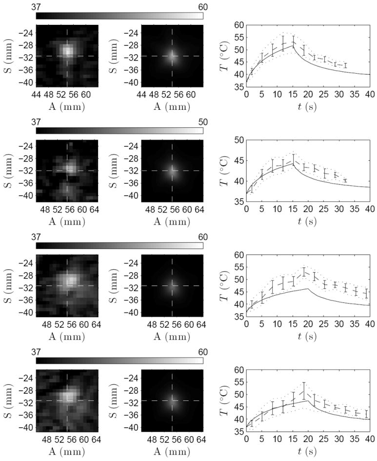
Left column: close-up of the measured thermal focus. Middle column: simulated temperature after spatial averaging over the MR-voxel volumes. The cross-section of dashed lines marks the prescribed target. Right column: temperature evolution for simulated (——), measured average (- - - -) with its standard deviation (vertical lines), and minimum and maximum temperatures (⋯⋯) in 3 × 3 voxel neighborhood centered at the peak temperature elevations. Data shown for sonications 1–4 from top to bottom in patient A.
Table 6.
The full-width half-maximum (FWHM) of the focal temperature elevation at the end of the sonication for each measured and simulated sonication, and the offset of the measured and simulated focus from the prescribed target. The parentheses after patient A are the sonication index. The values before the slash are FWHM in the anterior–posterior direction; after the slash, in the inferior–superior direction.
| Patient | Treatment FWHM (mm) | Treatment offset (mm) | Simulation FWHM (mm) | Simulation offset(mm) |
|---|---|---|---|---|
| A (1) | 4.1 / 4.5 | 1.1 | 3.3 / 4.1 | 0.2 |
| A (2) | 4.9 / 4.3 | 1.5 | 3.4 / 4.1 | 0.2 |
| A (3) | 6.8 / 5.2 | 2.4 | 3.6 / 4.3 | 0.5 |
| A (4) | 6.7 / 5.1 | 2.2 | 3.6 / 4.3 | 0.3 |
| B | 5.0 / 6.1 | 2.2 | 2.6 / 3.9 | 0.4 |
| C | 4.4 / 5.8 | 1.1 | 3.2 / 4.2 | 0.4 |
| D | 7.1 / 7.2 | 1.5 | 2.9 / 3.9 | 0.2 |
| E | 5.7 / 5.3 | 1.0 | 3.1 / 4.4 | 0.3 |
Figure 6 shows the close-up of the measured and simulated sonications in patients B through E. The simulated temperatures shown are averaged over the size of the MR voxels. The figure also shows the focal temperatures as a function of time at the peak temperature elevation of the simulation and measurement respectively. In patients B, C, and E, the peak temperature in the simulations were lower than in the treatments. Post-sonication, temperatures seem to decline faster in the simulations than in the treatments, as is the case with patient A. The offset of the peak temperature elevations with respect to the prescribed target are shown in Table 6.
Figure 6.
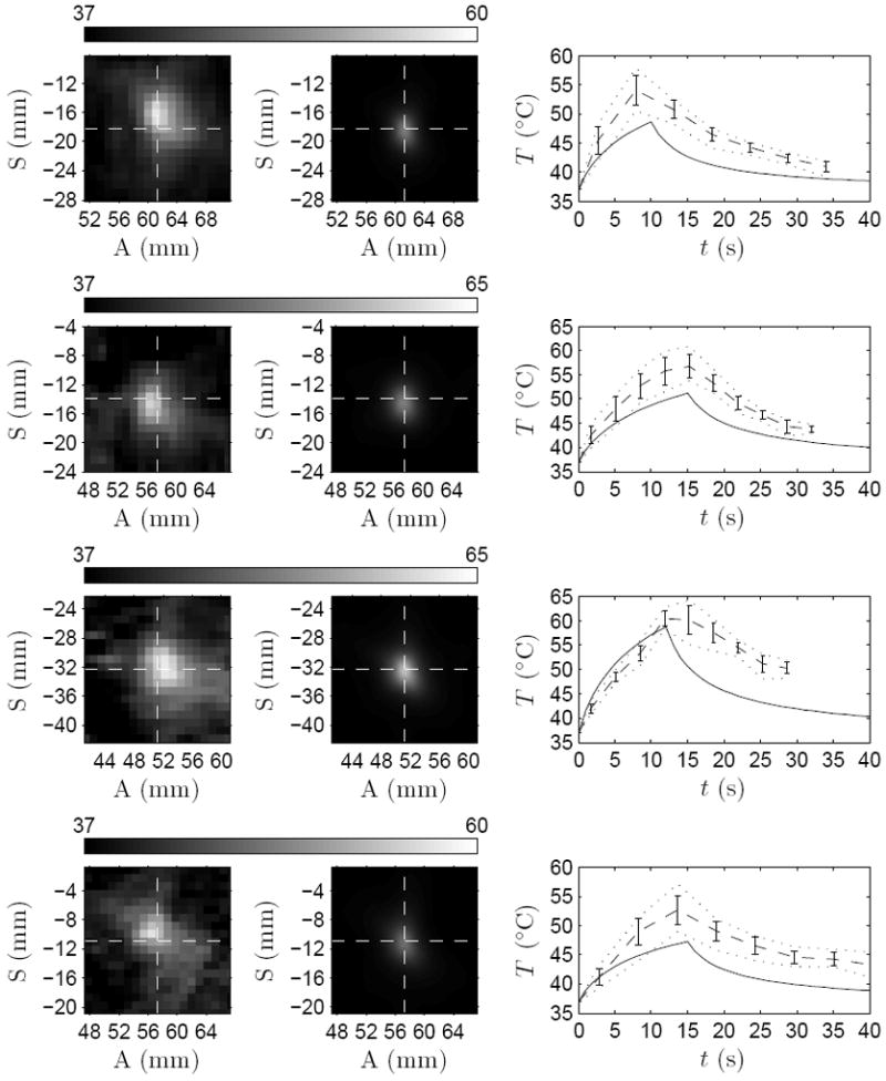
Left column: close-up of the measured thermal focus. Middle column: simulated temperature after spatial averaging over the MR-voxel volumes. The cross-section of dashed lines marks the prescribed target. Right column: temperature evolution for simulated (——), measured average (- - - -) with its standard deviation (vertical lines), and minimum and maximum temperatures (⋯⋯) in 3 × 3 voxel neighborhood centered at the peak temperature elevations. Data shown for sonications in patients B–E from top to bottom.
The measured and simulated temperatures at the end of the sonications are shown in Table 5 for each of the sonications. The analysis was performed at the center of the peak temperature elevation of the measurements and the simulations, respectively. On average, the simulated temperature elevations were 24 ± 13 % lower than the measured temperature elevations in patients A through E. The peak temperature elevations of the simulations and measurements differed from the prescribed location, as shown in Table 6. On average the treatments resulted in a peak temperature elevation offset of 1.6 ± 0.6 mm from the prescribed target, while the simulations were off by 0.3 ± 0.1 mm.
Table 6 shows the full-width half-maximum (FWHM) for the focal temperature elevation computed for all treatments and simulations. FWHM is shown for anterior–posterior (AP) and inferior–superior (IS) directions. On average, the simulations resulted in 40 ± 13% smaller thermal foci in AP direction and 22 ± 14% in IS direction for patients A through E than those measured in the treatments.
The effect of variations of some of the simulation parameters on the simulation results are demonstrated in Figure 7. The figure shows the effect that phase-correction, blood perfusion, simulating the skull as either fluid or solid, skull attenuation and skull sound speed have on the focal temperatures. The simulations in the figure were performed using the geometry and sonication parameters of sonication one in patient A.
Figure 7.
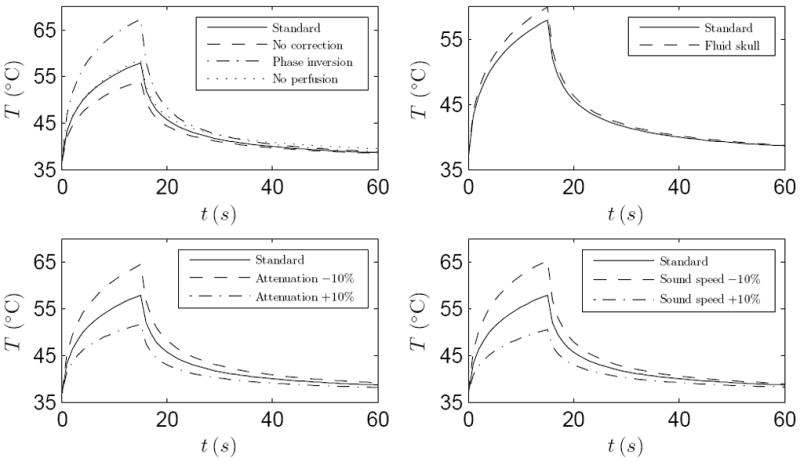
Focal temperatures with varied simulation parameters performed on the geometry and baseline parameters of patient A and sonication one. Shown in each figure is the baseline simulation with standard parameters (——). Top left: simulation with no phase correction (- - - -), simulation with phase inversion (— · —) and simulation with no blood perfusion (⋯⋯). Top right: simulation with skull modeled as fluid (- - - -). Bottom left: simulations with skull attenuation decreased (- - - -) and increased (— · —) by 10%. Bottom right: simulations with skull sound speed decreased (- - - -) and increased (— · —) by 10%.
When the phase aberration caused by the skull is ignored, the focal temperature elevation is reduced by 18 % in comparison to simulation with the treatment phasing, however the focus is shifted by 1.2 mm away from the prescribed target. When, on the other hand, a phase inversion is performed (this is achieved by placing a point source at the focus, simulating the propagation of ultrasound from the point source to the phased array, inverting the recorded ultrasound phase on the phased array, and re-emitting the sound wave at the inverted phase), the focal temperature elevation increased by 45 %.
Ignoring the blood perfusion results in a temperature elevation that is 4 % higher than when using the blood perfusion in Table 4. The blood perfusion also slightly affects the rate at which the focal temperature returns to the baseline temperature.
Modeling the skull as a fluid instead of solid will result in overestimation of 9 % in focal temperature elevation. Decreasing the longitudinal and shear wave attenuation by 10% resulted in a focal temperature elevation increase of 30%, whereas increasing the attenuation by 10% resulted in a focal temperature elevation decrease of 32%. Similarly, decreasing the longitudinal and shear sound speeds by 10% resulted in a focal temperature elevation increase of 35%, whereas increasing the sound speeds by 10% resulted in a focal temperature elevation decrease of 35%.
4. Discussion
A hybrid simulation model using a grid and a finite difference method to solve the fluid and solid wave equations was developed to simulate ultrasound propagation in transcranial ultrasound therapy. Simulation geometry was derived from five patient treatments and the treatment sonications were simulated with the sonication phase and amplitude used in the treatments. The simulated ultrasound fields and both simulated and measured temperature fields were investigated for each of the patients.
The temperature elevations predicted by the simulations were on average 24±13% lower than the measured temperature elevations. The position of the simulated focus matched the prescribed location well with an average offset of 0.3±0.1mm. However, the treatment sonications were on average 1.6±0.6 mm off from the prescribed target. The reason that the simulation matched with the prescribed target so well, in comparison to the measurements, could be that the phase correction employed by the clinical system utilizes similar material parameters and the same geometry as used in the simulations to perform the phase calculation. If the true acoustical properties of the patient (namely those of the skull and the soft-tissue) were to differ from the parameters used by the phase correction algorithm, an offset would occur.
In one sonication location and patient geometry, the effect of a few crucial parameters affecting the simulations was also investigated. Ignoring the phase correction resulted in shifted and reduced temperature elevation at the focus, while using phase inversion resulted in an elevation of the focal temperature. Blood perfusion, on the other hand, was found to have only a small effect on the focal temperature elevation. Using a simplified simulation model, with the skull modeled as fluid, resulted in overestimation of the focal temperature in comparison to the simulation model where the skull was modeled as a solid. This is due to lower total absorption of the transmitted wave with the fluid model, as no mode-conversion of the pressure wave to shear wave (higher attenuation) takes place, and only the longitudinal wave attenuation mechanisms attenuate the wave. It is expected, however, that when the sonication location is shifted farther away from the central areas of the brain, or when the transducer is placed such that the ultrasound is transmitted mostly at an oblique angle with respect to the skull, the significance of modeling the skull as a solid is increased [33].
Decreasing or increasing the longitudinal and shear skull attenuation by 10% resulted in an increase or decrease of the focal temperature elevation by 30% and 32% respectively. When the longitudinal and shear sound speeds were decreased or increased by 10% the focal temperature elevation increased or decreased by 35% respectively. This result can be explained by the acoustical impedance of the skull being more similar to that of water and soft tissue when the sound speeds are decreased, thus resulting in a higher transmission of ultrasound through the skull.
These results demonstrate the impact of the acoustic properties of the skull on the predicted temperature elevation and indicate that the uncertainties in the values used in this study may be the reason for the deviations between the simulated and measured temperature elevations. They also indicate strongly that we need better knowledge of the acoustical properties of the human skull.
The model used to compute the longitudinal sound speed and attenuation of the skull as a function of density in [34], the source for the acoustical parameters of the skull in this study, does not completely incorporate wave propagation of solids. As a consequence, it might be possible that the actual longitudinal sound speeds differ from the values used. In addition, although the measurements were done using normal incidence between the ultrasound beam and the skull surface, the neglection of shear waves when estimating the longitudinal attenuation in solids might result in overestimation of the attenuation. This would reflect in this study as too high of attenuation for waves transmitting through the skull, resulting in reduced focal pressure, and thus, absorbed power density and temperature.
Other potential reasons for the underestimation of the temperature when using the treatment phasing include numerical phase dispersion, enhanced heating at the focus, and inaccuracies in simulation geometry.
Numerical phase dispersion causes simulated waves to propagate at different speeds than the sound speed. This could result in reduced focal pressure amplitude because the phases are not ideally corrected, if the dispersion is not taken into account.
It could, as well, be that the thalamus has a higher ultrasound absorption coefficient than the one used in this study. This would enhance conversion of pressure into heat and elevate the focal temperature.
The slow, almost linear, decay of the measured temperatures after the sonications, in comparison with the simulated temperatures, would indicate that the Laplacian term in equation (3) does not have a big influence at the focus. This could be a result of either the overestimated value of thermal conductivity used in the simulations or a change in the thermal conductivity during the sonication. Another source that would result in reduced impact of the Laplacian in thermal simulations would be spatially wider Q, and hence, spatially wider T. An argument supporting this is the larger size of the thermal focus in the measurements when compared to simulations. Differences in the spatial extent of the thermal focus between the measurements and simulations could be a result of, for example, additional heating mechanisms which might be arising from cavitation effects [4]. Another explanation could be that the skull bone structure is introducing ultrasound scattering and distortion in each of the ultrasound beams generated by individual phased array elements. The impact of the actual bone structure in the beam propagation is currently not known and should be a subject of a further study.
The three main differences between the simulation and the treatment geometries are the exact shape and size of each phased array element, the membrane covering the aperture of the transducer in the treatments, and the assumption of negligible soft-tissue heterogeneities inside the brain. The unknown shape of the phased array elements would result in slight differences in the simulated pressure fields when compared with the measurements. The shape also affects the directivity pattern of each element and could have an impact on the focal gain of the simulated phased array. In the treatments, a membrane was used to allow partial immersion of the head inside the transducer. In the simulations, however, the membrane was neglected, as its exact shape and position is hard to be determined. The effect that the membrane could have on the focus is most likely minimal: the reflection of sound caused by the membrane far away from the focus and well outside the directivity pattern of the phased array elements is small. The reflection taking place on the membrane would also most likely be directed away of the focus, essentially reducing the reflected beams amplitude to negligible level in terms of the focal pressure. The heterogeneities of the soft tissue were neglected for simplicity, although the presented simulation model would allow to incorporate them into the geometry. As the variability of the acoustic parameters in soft tissues is small, it is expected that the impact of these heterogeneities on the results presented would be small. On the other hand heterogeneities could lead to increase in the amount of scattering of ultrasound taking place on the interfaces between different soft tissue regions. This could increase the size of the focal volume and thus potentially reduce the discrepancy between the simulations and the treatments. It may also reduce the peak temperature elevation thus increasing the difference observed in this aspect.
In addition, the acoustic power values used in the simulations were based on the numbers given by the system. This number is based on the measured RF power during the sonication and it is not known how well the conversion efficiency of each of the transducer elements was calibrated for each of the sonications. The accuracy of current ultrasound lab equipment for this kind of calibration is in the range of 5 – 10 % [41]. Therefore it can be assumed that the calibration of the total acoustic power could be off by a factor of 10 % and perhaps more, because of the hemispherical shape of the array which complicates the calibration. Similarly, we do not know how much variation there is between the elements and how stable the calibration is.
Finally, the ultrasound beam reflected from the outer skull surface back to the transducer face can have an impact on the impedance of the transducer elements, its power output, and perhaps on the transmitted phase as well [7]. Since this effect is dependent on the distance between the skull and the transducer element its impact will vary from element to element, and its magnitude to the overall sonication is difficult to determine at this stage.
As a conclusion, the simulation model developed here can predict the location of the focal spot achieved in clinical treatments. Although the actual temperature elevation and the size of the focal spot were under-predicted, the model can give useful guidance when patient treatments are planned, or when new devices are designed, or when treatment schemes are investigated. The model could also work as a valuable tool in the treatment planning, when assessment of feasibility of treatment is evaluated. The results would call for more thorough investigation of the material parameters affecting the transcranial treatment, namely the acoustical parameters of the skull and the thermal parameters of the soft tissues. Both of these parameters are important factors in successful treatment planning and in understanding the physics involved. Accurate acoustical properties of the skull could be utilized to develop improved phasing algorithms resulting in more efficient sonications. Accurate thermal parameters, on the other hand, would allow estimation of the sonication parameters needed to achieve desired temperature and thermal dose in the target. Both of these factors would increase the speed and quality of ultrasound treatments of the brain.
Acknowledgments
The authors wish to thank the Finnish IT Center for Science (CSC) for computational resources. This work was supported by grants from the National Institutes of Health (No. R01EB003268) and the Canada Research Chair program (CRC).
Appendix
The computational model used in this paper solves the acoustic wave equations of fluid and solid. The model utilizes grid method (GM) [44] and finite difference (FD) method. GM is used due to its flexibility to handle complex fluid–solid interfaces, whereas FD is used due to its lower numerical dispersion. The computational geometry is presented in Cartesian grid form with cubical elements of side-length Δh. Each element is defined to be either fluid or solid with corresponding material parameters. Grid nodes are located at the corners of each element.
Computation of GM proceeds utilizing integral formulations of the wave equations
| (A.1) |
| (A.2) |
where V is the integrated volume surrounded by closed surface S, n is the surface normal and τ is the stress tensor defined as
| (A.3) |
Integrated volume V is the control volume surrounding any given grid node in the computational domain that is a cube of side length Δh centered on the grid node. The control volume is depicted in Figure A1a in 2D case.
Left hand side of the equations (A.1) and (A.2) are mass-lumped such that the acoustical fields are presumed constant in the integrated volume resulting in approximations
| (A.4) |
| (A.5) |
where integers i, j, k refer to grid-node indices in x–, y–, and z–axes.
On the right hand side of equations (A.1) and (A.2) the acoustic field f (either p or u) is approximated using the sum of linear basis functions as
| (A.6) |
where fn are values of the acoustic field at the corners of an element and ϕn are the basis functions corresponding to these corners. Basis functions ϕn are mapped from basis functions defined for the basis element spanning volume of [−1, 1] × [−1, 1] × [−1, 1] as
| (A.7) |
| (A.8) |
| (A.9) |
| (A.10) |
| (A.11) |
| (A.12) |
| (A.13) |
| (A.14) |
| (A.15) |
Mapping between ϕn (x,y,z) and is done using , where (x0, y0, z0) are the coordinates of the element. The linear approximation allows solving of the surface integrals analytically.
FD method can be written using the presented integral equations by changing the definition of basis functions by
| (A.16) |
The result is discontinuous basis functions for which the spatial derivative terms have to be approximated. As the derivatives are only required on the surface of the control volume, they can be approximated with centered finite differences. Figure A1b shows how the differences would be approximated in 2D. 3D extension is done similarly.
Splitting the simulation geometry into domains where GM and FD methods are used is done by following a few rules. All elements that are part of fluid–solid interface are considered to be GM elements. All other elements are considered as FD elements. If a grid node is surrounded by GM elements, then the grid node is computed using GM method. If a grid node is surrounded by FD elements, then FD method is used. For grid nodes surrounded by both GM and FD elements, coupling of the two models is required.
Coupling between the GM and FD methods is done with the integral formulation. When performing computation for a grid node and integrating over the control volume’s surface S, the integral is split into eight sub-integrals corresponding to integrals over the intersections of S and the elements surrounding the grid node. If any of these elements is considered to be GM or FD elements as described above, then the corresponding basis functions and derivative estimations are used.
FD nodes that are surrounded by other FD nodes are computed by discretizing equations (1) and (2) directly with centered second and fourth order derivative approximations. FD nodes which are surrounded by 3 × 3 × 3 neighborhood of FD nodes are computed using second-order centered finite differences. Nodes that have FD nodes in neighborhoods of 5 × 5 × 5 are computed using fourth-order centered finite differences.
The temporal integration is done using second-order centered in time FD method for the pressure wave equation. For solid nodes the temporal integration is done by using two-step predictor-correction method of form
| (A.17) |
| (A.18) |
where L and G are the spatial difference operators operating on either the discretized field quantity yn or FD estimate of its temporal derivative, and ỹn+1 is the predicted field on the integrated time step, and yn+1 is the corrected time step. The method was used for its computational performance over implicit temporal integration methods that would arise from the viscosity terms of the solid wave-equation.
The derivative approximations used with finite differences are for the first derivative
| (A.19) |
for second-order accuracy and
| (A.20) |
for fourth-order accuracy. Second derivatives are approximated with
| (A.21) |
for second-order accuracy and
| (A.22) |
for fourth-order accuracy. In the above, Δ is either the temporal discretization Δt or spatial discretization Δh.
Figure A1.
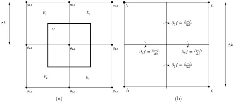
a) 2D grid composed of four elements El with grid node gi,j and the control volume V associated with grid node g2,2. b) Computation of finite difference derivative approximations in basis element using FD method in 2D.
References
- 1.Aubry J-F, Tanter M, Pernot M, Thomas J-L, Fink M. Experimental demonstration of noninvasive transskull adaptive focusing based on prior computed tomography scans. J Acoust Soc Am. 2003;113(1):84–93. doi: 10.1121/1.1529663. [DOI] [PubMed] [Google Scholar]
- 2.Auld BA. Acoustic Fields and Waves in Solids vols 1 and 2. Wiley; New York: 1973. [Google Scholar]
- 3.Baron C, Aubry J-F, Tanter M, Meairs S, Fink M. Simulation of intracranial acoustic fields in clinical trials of sonothrombolysis. Ultrasound Med Biol. 2009;35(7):1148–58. doi: 10.1016/j.ultrasmedbio.2008.11.014. [DOI] [PubMed] [Google Scholar]
- 4.Chavrier F, Chapelon JY, Gelet A, Cathignol D. Modeling of high-intensity focused ultrasound-induced lesions in the presence of cavitation bubbles. J Acoust Soc Am. 108(1):432–40. 108. doi: 10.1121/1.429476. [DOI] [PubMed] [Google Scholar]
- 5.Clement GT, Hynynen K. Micro-receiver guided transcranial beam steering. IEEE Trans Ultrason Ferroelectr Freq Control. 2002;49(4):447–53. doi: 10.1109/58.996562. [DOI] [PubMed] [Google Scholar]
- 6.Clement GT, Hynynen K. A non-invasive method for focusing ultrasound through the human skull. Phys Med Biol. 2002;47:1219–36. doi: 10.1088/0031-9155/47/8/301. [DOI] [PubMed] [Google Scholar]
- 7.Clement GT, Sun J, Hynynen K. The role of internal reflection in transskull phase distortion. Ultrasonics. 2001;39:109–113. doi: 10.1016/s0041-624x(00)00052-4. [DOI] [PubMed] [Google Scholar]
- 8.Clement GT, White J, Hynynen K. Investigation of a large-area phased array for focused ultrasound surgery through the skull. Phys Med Biol. 2000;45:1071–83. doi: 10.1088/0031-9155/45/4/319. [DOI] [PubMed] [Google Scholar]
- 9.Clement GT, White PJ, Hynynen K. Enhanced ultrasound transmission through the human skull using shear mode conversion. J Acoust Soc Am. 2004;115(3):1356–64. doi: 10.1121/1.1645610. [DOI] [PubMed] [Google Scholar]
- 10.Connor CW, Clement GT, Hynynen K. A unified model for the speed of sound in cranial bone based on genetic algorithm optimization. Phys Med Biol. 2002;47:3925–44. doi: 10.1088/0031-9155/47/22/302. [DOI] [PubMed] [Google Scholar]
- 11.Connor CW, Hynynen K. Bio-acoustic thermal lensing and nonlinear propagation in focused ultrasound surgery using large focal spots: a parametric study. Phys Med Biol. 2002;47:1911–28. doi: 10.1088/0031-9155/47/11/306. [DOI] [PubMed] [Google Scholar]
- 12.Connor CW, Hynynen K. Patterns of thermal deposition in the skull during transcranial focused ultrasound surgery. IEEE Trans Biomed Eng. 2004;51(10):1693–708. doi: 10.1109/TBME.2004.831516. [DOI] [PubMed] [Google Scholar]
- 13.Cooper TE, Tezek GJ. A probe technique for determining the thermal conductivity of tissue. J Heat Transfer. 1972;94:133–40. [Google Scholar]
- 14.Croft DR. Heat Transfer Calculations Using Finite Difference Equations. Applied Science Publishers; London: 1977. [Google Scholar]
- 15.Deffieux T, Konofagu EE. Numerical study of a simple transcranial focused ultrasound system applied to blood-brain barrier opening. IEEE Trans Ultrason Ferroelectr Freq Control. 2010;57(12):2637–53. doi: 10.1109/TUFFC.2010.1738. [DOI] [PMC free article] [PubMed] [Google Scholar]
- 16.Dillenseger J-L, Esneault S. Fast fft-based bioheat transfer equation computation. Comput Biol Med. 2010;40:119–23. doi: 10.1016/j.compbiomed.2009.11.008. [DOI] [PubMed] [Google Scholar]
- 17.Duck F. Physical Properties of Tissue: A Comprehensive Reference. Academic; London: 1990. [Google Scholar]
- 18.Elias WJ, Huss D, Voss T, Loomba J, Khaled M, Zadicario E, Frysinger RC, Sperling SA, Wylie S, Monteith SJ, Druzgal J, Shah BB, Harrison M, Wintermark M. A pilot study of focused ultrasound thalamotomy for essential tremors. N Engl J Med. 2013;369:640–648. doi: 10.1056/NEJMoa1300962. [DOI] [PubMed] [Google Scholar]
- 19.Etame AB, Diaz RJ, Smith CA, Mainprize TG, Hynynen K, Rutka JT. Focused ultrasound disruption of the blood-brain barrier: a new frontier for therapeutic delivery in molecular neurooncology. Neurosurg Focus. 2012;32(1) doi: 10.3171/2011.10.FOCUS11252. [DOI] [PMC free article] [PubMed] [Google Scholar]
- 20.Gâteau J, Marsac L, Pernot M, Aubry J-F, Tanter M, Fink M. Transcranial ultrasonic therapy based on time reversal of acoustically induced cavitation bubble signature. IEEE Trans Biomed Eng. 2010;57(1):134–44. doi: 10.1109/TBME.2009.2031816. [DOI] [PMC free article] [PubMed] [Google Scholar]
- 21.Haworth KJ, Fowlkes JB, Carson PL, Kripfgans OD. Towards aberration correction of transcranial ultrasound using acoustic droplet vaporization. Ultrasound Med Biol. 2008;34(3):435–445. doi: 10.1016/j.ultrasmedbio.2007.08.004. [DOI] [PMC free article] [PubMed] [Google Scholar]
- 22.Hynynen K, McDannold N, Clement G, Jolesz FA, Zadicario E, Killiany R, Moore T, Rosen D. Pre-clinical testing of a phased array ultrasound system for mri-guided noninvasive surgery of the brain - a primate study. Eur J Radiol. 2006;59:149–56. doi: 10.1016/j.ejrad.2006.04.007. [DOI] [PubMed] [Google Scholar]
- 23.Jeanmonod D, Werner B, Morel A, Michels L, Zadicario E, Schiff G, Martin E. Transcranial magnetic resonance imaging-guided focused ultrasound: noninvasive central lateral thalamotomy for chronic neuropathic pain. Neurosurg Focus. 2012;32(1) doi: 10.3171/2011.10.FOCUS11248. [DOI] [PubMed] [Google Scholar]
- 24.Larrat B, Pernot M, Montaldo G, Fink M, Tanter M. Mr-guided adaptive focusing of ultrasound. IEEE Trans Ultrason Ferroelectr Freq Control. 2010;57(8):1734–47. doi: 10.1109/tuffc.2010.1612. [DOI] [PMC free article] [PubMed] [Google Scholar]
- 25.Lipsman N, Scwartz ML, Huang Y, Lee L, Sankar T, Chapman M, Hynynen K, Lozano AM. MR-guided focused ultrasound thalamotomy for essential tremor: a proof-of-concept study. Lancet Neurol. 2013;12:462–8. doi: 10.1016/S1474-4422(13)70048-6. [DOI] [PubMed] [Google Scholar]
- 26.Marquet F, Pernot M, Aubry J-F, Montaldo G, Marsac L, Tanter M, Fink M. Non-invasive transcranial ultrasound therapy based on a 3d ct scan: protocol validation and in vitro results. Phys Med Biol. 2009;54:2597–613. doi: 10.1088/0031-9155/54/9/001. [DOI] [PubMed] [Google Scholar]
- 27.Martin E, Jeanmonod D, Morel A, Zadicario E, Werner B. High-intensity focused ultrasound for noninvasive functional neurosurgery. Ann Neurol. 2009;66(6):858–61. doi: 10.1002/ana.21801. [DOI] [PubMed] [Google Scholar]
- 28.McDannold N, Clement GT, Black P, Jolesz F, Hynynen K. Transcranial magnetic resonance imaging-guided focused ultrasound surgery of brain tumors: initial findings in 3 patients. Neurosurgery. 2010;66(2):323–32. doi: 10.1227/01.NEU.0000360379.95800.2F. [DOI] [PMC free article] [PubMed] [Google Scholar]
- 29.McDannold N, Park E-J, Mei C-S, Zadicario E, Jolesz F. Evaluation of three-dimensional temperature distributions produced by a low-frequency transcranial focused ultrasound system within ex vivo human skulls. IEEE Trans Ultrason Ferroelectr Freq Control. 2010;57(9):1967–76. doi: 10.1109/TUFFC.2010.1644. [DOI] [PMC free article] [PubMed] [Google Scholar]
- 30.Medel R, Crowley RW, McKisic MS, Dumont AS, Kassell NF. Sonothrombolysis: an emerging modality for the management of stroke. Neurosurgery. 2009;65:979–93. doi: 10.1227/01.NEU.0000350226.30382.98. [DOI] [PubMed] [Google Scholar]
- 31.Pennes HH. Analysis of tissue and arterial blood temperatures in the resting human forearm. J Appl Physiol. 1948;1(2):93–122. doi: 10.1152/jappl.1948.1.2.93. [DOI] [PubMed] [Google Scholar]
- 32.Pernot M, Aubry J-F, Tanter M, Boch A-L, Marquet F, Kujas M, Seilhean D, Fink M. In vivo transcranial brain surgery with an ultrasonic time reversal mirror. J Neurosurg. 2007;106:1061–66. doi: 10.3171/jns.2007.106.6.1061. [DOI] [PubMed] [Google Scholar]
- 33.Pichardo S, Hynynen K. Treatment of near-skull brain tissue with a focused device usign shear-mode conversion: a numerical study. Phys Med Biol. 2007;52:7313–32. doi: 10.1088/0031-9155/52/24/008. [DOI] [PubMed] [Google Scholar]
- 34.Pichardo S, Sin VW, Hynynen K. Multi-frequency characterization of the speed of sound and attenuation coefficient for longitudinal transmission of freshly excised human skulls. Phys Med Biol. 2011;56:219–50. doi: 10.1088/0031-9155/56/1/014. [DOI] [PMC free article] [PubMed] [Google Scholar]
- 35.Pierce AD. Acoustics: An introduction to its Physical Principles and Applications. Acoustical Society of America Publications; Sewickley PA: 1989. [Google Scholar]
- 36.Pulkkinen A, Huang Y, Song J, Hynynen K. Simulations and measurements of transcranial low-frequency ultrasound therapy: skull-base heating and effective area of treatment. Phys Med Biol. 2011;(56):4661–83. doi: 10.1088/0031-9155/56/15/003. [DOI] [PubMed] [Google Scholar]
- 37.Song J, Pulkkinen A, Huand Y, Hynynen K. Investigation of standing-wave formation in a human skull for a clinical prototype of a large-aperture, transcranial mr-guided focused ultrasound (MRgFUS) phased array: an experimental and simulation study. IEEE Trans Biomed Eng. 2012;59(2):435–44. doi: 10.1109/TBME.2011.2174057. [DOI] [PMC free article] [PubMed] [Google Scholar]
- 38.Sun J, Hynynen K. Focusing of therapeutic ultrasound through a human skull: a numerical study. J Acoust Soc Am. 1998;104(3):1705–15. doi: 10.1121/1.424383. [DOI] [PubMed] [Google Scholar]
- 39.Tang SC, Clement GT. Acoustic standing wave suppression using randomized phase-shift-keying excitations. J Acoust Soc Am. 2009;126(4):1667–70. doi: 10.1121/1.3203935. [DOI] [PMC free article] [PubMed] [Google Scholar]
- 40.Tang SC, Clement GT. Standing-wave suppression for transcranial ultrasound by random modulation. IEEE Trans Biomed Eng. 2010;57(1):203–5. doi: 10.1109/TBME.2009.2028653. [DOI] [PMC free article] [PubMed] [Google Scholar]
- 41.ter Haar G, editor. The Safe Use of Ultrasound in Medical Diagnosis. 3. The British Institute of Radiology; London, UK: 2012. [Google Scholar]
- 42.Thomas JL, Fink MA. Ultrasonic beam focusin through tissue inhomogeneities with a time reversal mirror: application to transskull therapy. IEEE Trans Ultrason Ferroelectr Freq Control. 1996;43(6):1122–9. [Google Scholar]
- 43.White PJ, Clement GT, Hynynen K. Longitudinal and shear mode ultrasound propagation in human skull bone. Ultrasound Med Biol. 2006;32(7):1085–96. doi: 10.1016/j.ultrasmedbio.2006.03.015. [DOI] [PMC free article] [PubMed] [Google Scholar]
- 44.Zhang J. Wave propagation across fluid-solid interfaces: a grid method approach. Geophys J Int. 2004;159:240–52. [Google Scholar]