An Immersed Boundary Method for Two-fluid Mixtures

Abstract

We present an Immersed Boundary method for interactions between elastic boundaries and mixtures of two fluids. Each fluid has its own velocity field and volume-fraction. A penalty method is used to enforce the condition that both fluids’ velocities agree with that of the elastic boundaries. The method is applied to several problems: Taylor’s swimming sheet problem for a mixture of two viscous fluids, peristaltic pumping of a mixture of two viscous fluids, with and without immersed particles, and peristaltic pumping of a mixture of a viscous fluid and a viscoelastic fluid. The swimming sheet and peristalsis problems have received much attention recently in the context of a single viscoelastic fluid. Numerical results demonstrate that the method converges and show its capability to handle a number of flow problems of substantial current interest. They illustrate that for each of these problems, the relative motion between the two fluids changes the observed behaviors profoundly compared to the single fluid case.

1. Introduction

Interactions between elastic structures and a surrounding fluid medium are ubiquitous in biological processes, from the locomotion of E. coli in intestinal fluid to the swimming of sperm through cervical mucus. A powerful computational approach for handling this type of dynamic fluid structure interaction, in the case of single, incompressible fluids, is the Immersed Boundary (IB) method originally developed by Peskin [1]. The robustness of the IB method has led to its application in many different biofluid applications. For example, it has been used to study cardiac dynamics [2, 3, 4], platelet aggregation [5, 6], aquatic locomotion by small [7, 8] and large [9] organisms, cellular locomotion [10], peristalsis [11, 12] insect flight [13, 14], biofilms [15] and feeding by marine invertebrates [16, 17, 18]. It has also been used in a wide-range of engineering applications including, for example, electrohydrodynamics [19, 20] and reaction diffusion systems [21, 22]. In all of this work, the fluid environment is treated as a single continuous medium. However, many biological fluids such as mucus as well as many engineering and industrial fluids are mixtures of a solvent and a polymer network. There may be relative motion between the different components of the mixture and then describing the material as a single continuous medium is inappropriate. The two-fluid model is an often-used approach to describe gel mechanics, where both network and solvent coexist at each point of space, and each phase is modeled as a continuum with its own velocity field and constitutive law. Recently, analytical studies of G. I. Taylor’s classical swimming-sheet problem with two-fluid models have yielded interesting and unexpected results [23]. The analytical studies have been limited to simple geometries and small amplitude motions. In this paper, we present an extension of the classical immersed boundary method to a mixture of two fluids, in which both fluids satisfy the no-slip condition on the immersed structures. Enforcing this condition is one of the challenges in a two-fluid IB method. In the classic single-fluid IB method, the no-slip condition between the immersed boundary and the fluid is used to define the velocity of each point on the immersed structure as being the same as that of the adjacent fluid. In developing a two-fluid IB method, the question that arises is at which fluid’s velocity (or some average of them) points on the immersed boundary should move. Unless the two fluids have the same velocity at each point of the immersed structure, any of these choices for the velocity of the IB point is problematic and allows one or both fluids to move relative to the immersed structure. The key idea in our two-fluid IB method is to introduce two sets of immersed boundaries to represent the same elastic structure. Penalty forces are introduced to keep the boundaries moving at approximately the same velocity.

We apply the new method to three problems that illustrate its capabilities and demonstrate that accounting for relative motion between the two fluids can profoundly change the overall motion compared to the case of a single fluid. The first problem is that of determining the swimming speed of the classical Taylor’s undulating sheet in a mixture of two viscous fluids. For this problem, the motion of the undulating sheet is (approximately) imposed and the resulting fluid velocities, pressure, and volume-fractions are determined. As described in detail in [31], our simulations show that for two viscous fluids with different viscosities, the swimming speed is always less than for a single viscous fluid. Here we show the computed velocity fields and volume-fraction evolution, and we use this problem to numerically assess the convergence of the new method. For the second problem, we look at peristaltically-driven motion of a mixture of two viscous fluids. We see that the total flux driven by the peristalsis is greater for the mixture of fluids by an amount that depends on the ratio of the viscosities and on the composition (volume fractions) of the mixture. The flux is further altered by the presence of suspended elastic-walled particles. We also see two new aspects of the method’s performance: (i) the motion of the fluid (and suspended particles) within the tube is not sensitive to the composition of the fluid mixture outside of the tube, and (ii) the penalty forces are effective in ensuring that the network and solvent velocities are equal on the surfaces of the freely-moving suspended particles. For the third problem, we again look at peristalsis, but this time the network is viscoelastic and has time- and space-varying material properties that change as the system evolves. In this example, we see that network viscoelasticity and the possibility of relative motion between the solvent and the network have opposing effects on the net flux driven by the peristaltic motion.

The paper is organized as follows. In Section 2, we introduce the model equations and the numerical method. In Section 3.1, 3.2, and 3.3, we present, respectively, numerical simulations of Taylor’s swimming sheet problem for a mixture of two viscous fluids, simulations of peristaltic pumping of a mixture of two viscous fluids (both with and without immersed elastic particles), and simulations of peristaltic pumping of a fluid mixture composed of a viscoelastic network and a viscous solvent. Finally, in Section 4 we offer concluding remarks.

2. Model Equations and Numerical Method

Our development of a two-material immersed boundary method draws on our previous work on numerical methods for two-material mixtures [24] and on the immersed boundary methodology for a single fluid [1], so we begin this section by introducing the two-material model and reviewing the classical immersed boundary method.

2.1. Two-Material Mixture Model

We consider a mixture of two materials, which we denote ”solvent” and ”network”, in which both materials may be present at any spatial point x. While for some applications in this paper, the two materials are treated as immiscible viscous fluids, we use the solvent/network terminology throughout the paper for simplicity. The relative amounts of the two materials are given by the volume-fractions, θ^s(x, t) and θⁿ(x, t) for the solvent and network, respectively. We assume that the total amount of each material remains constant. The two volume-fractions evolve according to the continuity equations

$$\frac{\partial {\theta }^{\mathrm{n}}}{\partial t}+\nabla \cdot \left({\theta }^{\mathrm{n}}{\mathbf{u}}^{\mathrm{n}}\right)=0,$$ (1)

$$\frac{\partial {\theta }^{\mathrm{s}}}{\partial t}+\nabla \cdot \left({\theta }^{\mathrm{s}}{\mathbf{u}}^{\mathrm{s}}\right)=0.$$ (2)

where 0 < θⁿ < 1, θ^s = 1 – θⁿ and uⁿ(x, t) and u^s(x, t) are the network and solvent velocity respectively. Since θ^s + θⁿ = 1, adding these two equations gives an incompressibility constraint

$$\nabla \cdot ({\theta }^{\mathrm{n}}{\mathbf{u}}^{\mathrm{n}}+{\theta }^{\mathrm{s}}{\mathbf{u}}^{\mathrm{s}})=0.$$ (3)

on the volume-fraction averaged velocity θⁿuⁿ + θ^su^s.

The two velocity fields are determined from the momentum equations for the two materials. For this paper, we restrict our attention to the viscous-dominated situation in which inertial terms are ignored (similar to zero-Reynolds number flow) and in which the velocities and pressure respond instantaneously to applied forces. Under these conditions, the momentum equations reduce to the force-balance equations

$$\nabla \cdot \left({\theta }^{\mathrm{n}}\tau \right)+\nabla \cdot \left({\theta }^{\mathrm{n}}{\sigma }^{\mathrm{n}}\right)-\xi {\theta }^{\mathrm{n}}{\theta }^{\mathrm{s}}({\mathbf{u}}^{\mathrm{n}}-{\mathbf{u}}^{\mathrm{s}})-{\theta }^{\mathrm{n}}\nabla p+{\mathbf{f}}^{\mathrm{n}}=0,$$ (4)

$$\nabla \cdot \left({\theta }^{\mathrm{s}}{\sigma }^{\mathrm{s}}\right)-\xi {\theta }^{\mathrm{n}}{\theta }^{\mathrm{s}}({\mathbf{u}}^{\mathrm{s}}-{\mathbf{u}}^{\mathrm{n}})-{\theta }^{\mathrm{s}}\nabla p+{\mathbf{f}}^{\mathrm{s}}=0.$$ (5)

Here, τ is the viscoelastic stress tensor for the polymer network. σⁿ and σ^s are the viscous stress tensors for the network and solvent, respectively, ξθⁿθ^s(uⁿ – u^s) describes the frictional drag between the two phases (where ξ > 0 is the drag coefficient), and p is the pressure. The network and solvent force densities fⁿ and f^s are generated by the immersed elastic structures as described in detail below. The viscous stress tensors σⁿ and σ^s are taken to be those for Newtonian fluids:

$${\sigma }^{\mathrm{n}}={\mu }_{\mathrm{n}}\left(\nabla {\mathbf{u}}^{\mathrm{n}}+\nabla {\mathbf{u}}^{\mathrm{n}T}\right)+\left({\lambda }_{\mathrm{n}}\nabla \cdot {\mathbf{u}}^{\mathrm{n}}\right)I$$ (6)

$${\sigma }^{\mathrm{s}}={\mu }_{\mathrm{s}}\left(\nabla {\mathbf{u}}^{\mathrm{s}}+\nabla {\mathbf{u}}^{\mathrm{s}T}\right)+\left({\lambda }_{\mathrm{s}}\nabla \cdot {\mathbf{u}}^{\mathrm{s}}\right)I.$$ (7)

Here I is the identity tensor, μ_n,s are the shear viscosities and λ_n,s + 2μ_n,s/d are the bulk viscosities of the network and solvent (d is the dimension), and I is the identity tensor. We choose λ_n,s = –μ_n,s so that the bulk viscosities in both phases are zero.

For the example with a viscoelastic network, we have in mind a transient network in which the elastic links comprising the network form and break dynamically. We describe the strength of the network at any time t and location x by the quantity z(x, t), which satisfies the equation

$$z_t+\nabla \cdot \left({\mathbf{u}}^{\mathrm{n}}z\right)=\alpha \left({\theta }^{\mathrm{n}}\right)-\beta z,$$ (8)

where α and β are the link formation and breaking rates, respectively. The variable z is proportional to the density of crosslinks present. The network viscoelastic stress tensor evolves according to the constitutive equations

$${\tau }_t+\nabla \cdot \left({\mathbf{u}}^{\mathrm{n}}\tau \right)-(\tau +\mathit{zI})\nabla {\mathbf{u}}^{\mathrm{n}}-\nabla {\mathbf{u}}^{\mathrm{n}T}(\tau +\mathit{zI})=-\beta \tau .$$ (9)

We define the polymer relaxation time κ

$$\kappa ={\beta }^{-1},$$ (10)

and polymer viscosity μ_p

$${\mu }_p=z\kappa .$$ (11)

The elastic modulus of the network μ_p/κ is a function of z. We are modeling the network as an Oldroyd-B fluid with spatially and temporally varying elastic modulus. See [24] for a more detailed discussion of the model.

2.2. Classical Immersed Boundary Method

The “classical” Immersed Boundary method deals with the coupled motion of a single viscous incompressible fluid and one or more elastic objects in contact with the fluid. An Eulerian description is used for the fluid and the fluid dynamics are described by the incompressible Navier-Stokes equations with a force density contribution from each of the elastic objects

$$\rho \left({\mathbf{u}}_t+\mathbf{u}\cdot \nabla \mathbf{u}\right)=-\nabla p+\mu \Delta \mathbf{u}+\mathbf{f}\nabla \cdot \mathbf{u}=0.$$ (12)

Here, u(x, t), p(x, t) are the unknown fluid velocity and pressure, μ and ρ are the fluid’s viscosity and density, and f is the total force density generated by the immersed elastic objects.

A Lagrangian description is used for each immersed elastic object. For the case of a single one-dimensional object in a two-dimensional fluid, the locations of points on the object at time t are given by X(q, t) where q parameterizes material points on the object. Using a prescribed constitutive relation, a force (per unit q) is computed at each point of the elastic object from the function X(q, t)

$$\mathbf{F}(q,t)=\mathcal{F}\left(\mathbf{X}\right(\cdot ,t),q,t).$$ (13)

The coupling between the fluid and the object is accomplished through two integral relations

$$\mathbf{f}(\mathbf{x},t)={\int }_{\text{object}}\mathbf{F}(q,t)\delta (\mathbf{x}-\mathbf{X}(q,t\left)\right)\mathit{dq},$$ (14)

and

$$\frac{d\mathbf{X}}{\mathit{dt}}(q,t)={\int }_{\text{fluid}}\mathbf{u}(\mathbf{x},t)\delta (\mathbf{x}-\mathbf{X}(q,t\left)\right)d\mathbf{x},$$ (15)

in which δ denotes a two-dimensional Dirac delta function. The first of these equations describes how the force F at each point of the object is transmitted to the fluid, and the second expresses the assumption that each point of the immersed object moves at the local fluid velocity (this is the no-slip condition).

In calculations, discrete versions of Equations (12)-(15) are used. Typically, a Cartesian grid and finite-difference approximation are used for the fluid dynamics equations (12), the integrals in equations (14)-(15) are approximated by discrete sums in which the Dirac delta function is replaced by a regularized “approximate” delta function of finite support, and the Lagrangian point locations are updated using a discrete-time approximation to Equation (15). Detailed discussion of the immersed boundary method including the approximate delta-functions can be found in [1]. We note that in some applications of the method in which the viscosity is dominant, the Navier-Stokes equations (12) are replaced by the Stokes equations [5, 25].

One reason that the IB method has found wide applicability is the freedom in choosing the force-generating rules used in Equation (13). Various rules have been used to give the objects desired resistance to stretch or bending [7, 26]. Using elastic springs to “tether” IB points to target points whose motion is specified, a desired motion can be defined for each immersed boundary while still allowing it to respond appropriately to the hydrodynamics [14, 18, 16]. By allowing the connections between IB points to form and break dynamically, transient cell-cell adhesion and viscoelastic network dynamics have been studied [10, 5]. This flexibility extends to the two-fluid Immersed Boundary method we introduce in this paper.

2.3. Two-fluid Immersed Boundary Method

In thinking about extending the classical Immersed Boundary method to a two-material mixture, one faces two new issues. At what velocity should the points on an immersed object move? How should the Immersed Boundary forces generated at the IB points be distributed to the two materials? The answers to these questions depend on what physical conditions one is trying to capture. In this paper, we consider the case where both materials are to satisfy the no-slip condition at each point of the immersed object. In the classical IB method the way the no-slip condition is enforced is through Equation (15), which defines the velocity at each IB point so that the no-slip condition is satisfied by definition. In the present two-fluid case, if the solvent and network velocities were equal at each point of an immersed object, then this approach would work here as well. However, it is not obvious how to enforce this equality of the velocities in the IB context. If the solvent and network velocities differ at an IB point, then, clearly, one cannot make both fluids satisfy the no-slip condition at that point. Our approach to overcoming this challenge is to use two immersed boundaries for each immersed object, one of which “communicates” with each of the two fluids. Points on the “solvent” immersed boundary move according to the analog of Equation (15) with the solvent velocity u^s used in the integral, and, similarly, points on the “network” immersed boundary move according to the analog of Equation (15) with the network velocity uⁿ used in the integral. By definition then, each fluid satisfies a no-slip condition with respect to the corresponding immersed boundary. The second component of this approach is to introduce penalty forces that act on the corresponding points of the two immersed boundaries to oppose motions that move them apart. The details of our two-fluid IB method follow.

As in the standard IB method, we use an Eulerian description of the fluid variables, in this case for each of the two fluids, and we use a Lagrangian description for each of the immersed boundaries. For each immersed structure, we introduce two immersed boundaries, which we denote Γⁿ and Γ^s, as shown in Fig. 1. The locations of points on the solvent and network immersed boundaries are given, respectively, by the vector functions Xⁿ(q, t) and X^s(q, t), with Xⁿ(q, 0) = X^s(q, 0). Each Lagrangian point on Γⁿ communicates only with the network and each Lagrangian point on Γ^s communicates only with the solvent. In particular, the velocity of an IB point on Γⁿ is determined by the local network velocity field uⁿ, while the velocity of an IB point on Γ^s is determined by the local solvent velocity u^s. These velocities are specified by formulas similar to Equation (15) as described below.

Figure 1.

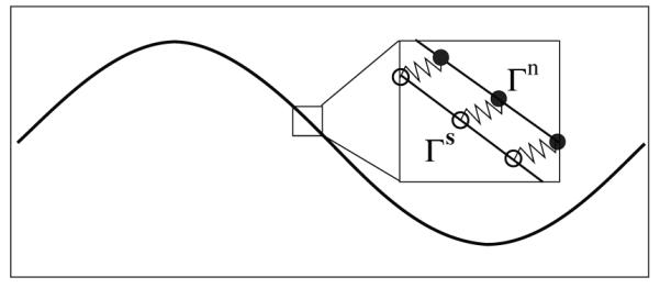
Dual IB representation of an immersed surface.

The forces at each Lagrangian point are of several types. Each point is connected by linear springs to its two neighboring points on the same immersed boundary. These spring forces specify the immersed boundary’s internal elastic properties. Each point on Γⁿ is connected by a stiff spring to the corresponding point on Γ^s. These springs generate “penalty forces” when the points they connect are at different locations. Each point on Γⁿ is also connected by a stiff spring to a corresponding “tether” point. By imposing the motion of the tether points, we can drive the motion of Γⁿ. Similarly, each point on Γ^s is connected to a tether point whose motion we impose.

Each force on Γⁿ is distributed to the surrounding network fluid as in the classical IB method using an analog of Equation (14), and similarly forces on Γ^s are transmitted to the solvent. However, the different distributed forces are weighted differently so it is convenient to distinguish the penalty force ${\mathbf{F}}_p^{\mathrm{n},\mathrm{s}}$ on the two immersed boundaries from the other forces ${\mathbf{F}}_o^{\mathrm{n},\mathrm{s}}$, that is, the sum of the elastic and tether forces. After they are transmitted to the fluid, the penalty forces are scaled by the product of the volume-fractions θⁿθ^s. This ensures that there is no interphase penalty force if either of the volume fractions goes to zero, and it ensures that equal and opposite penalty forces are applied to the solvent and the network since ${\mathbf{F}}_p^{\mathrm{n}}=-{\mathbf{F}}_p^{\mathrm{s}}$. The forces within each phase are scaled by that phase’s volume-fraction. With these understandings, the momentum equations for the network and solvent, respectively, are:

$$\nabla \cdot \left({\theta }^{\mathrm{n}}\tau \right)+\nabla \cdot \left({\theta }^{\mathrm{n}}{\sigma }^{\mathrm{n}}\right)-\xi {\theta }^{\mathrm{n}}{\theta }^{\mathrm{s}}({\mathbf{u}}^{\mathrm{n}}-{\mathbf{u}}^{\mathrm{s}})-{\theta }^{\mathrm{n}}\nabla p+{\theta }^{\mathrm{n}}{\mathbf{f}}_o^{\mathrm{n}}+{\theta }^{\mathrm{n}}{\theta }^{\mathrm{s}}{\mathbf{f}}_p^{\mathrm{n}}=0,$$ (16)

$$\nabla \cdot \left({\theta }^{\mathrm{n}}\tau \right)+\nabla \cdot \left({\theta }^{\mathrm{n}}{\sigma }^{\mathrm{n}}\right)-\xi {\theta }^{\mathrm{n}}{\theta }^{\mathrm{s}}({\mathbf{u}}^{\mathrm{n}}-{\mathbf{u}}^{\mathrm{s}})-{\theta }^{\mathrm{n}}\nabla p+{\theta }^{\mathrm{n}}{\mathbf{f}}_o^{\mathrm{n}}+{\theta }^{\mathrm{n}}{\theta }^{\mathrm{s}}{\mathbf{f}}_p^{\mathrm{n}}=0,$$ (17)

As in Section 2.1, the variable τ is the viscoelastic stress tensor. σⁿ and σ^s are the viscous stress tensors for the network and solvent, ξθⁿθ^s(uⁿ – u^s) describes the friction drag between the two phases, and p is the pressure. The new quantities in these equations are the contributions θⁿθ^s${\mathbf{f}}_p^{\mathrm{n}}$ and θⁿθ^s${\mathbf{f}}_p^{\mathrm{s}}$ to the force densities from the penalty forces, and the contributions ${\theta }^{\mathrm{n}}{\mathbf{f}}_o^{\mathrm{n}}$ and ${\theta }^{\mathrm{s}}{\mathbf{f}}_o^{\mathrm{s}}$ from the elastic and tether forces. The force densities in the momentum equations are defined from the Lagrangian force densities by the integral relations

$$\nabla \cdot \left({\theta }^{\mathrm{n}}\tau \right)+\nabla \cdot \left({\theta }^{\mathrm{n}}{\sigma }^{\mathrm{n}}\right)-\xi {\theta }^{\mathrm{n}}{\theta }^{\mathrm{s}}({\mathbf{u}}^{\mathrm{n}}-{\mathbf{u}}^{\mathrm{s}})-{\theta }^{\mathrm{n}}\nabla p+{\theta }^{\mathrm{n}}{\mathbf{f}}_o^{\mathrm{n}}+{\theta }^{\mathrm{n}}{\theta }^{\mathrm{s}}{\mathbf{f}}_p^{\mathrm{n}}=0,$$ (18)

where j = n, s and i = o, p. The final equations which close the system are

$$\nabla \cdot \left({\theta }^{\mathrm{n}}\tau \right)+\nabla \cdot \left({\theta }^{\mathrm{n}}{\sigma }^{\mathrm{n}}\right)-\xi {\theta }^{\mathrm{n}}{\theta }^{\mathrm{s}}({\mathbf{u}}^{\mathrm{n}}-{\mathbf{u}}^{\mathrm{s}})-{\theta }^{\mathrm{n}}\nabla p+{\theta }^{\mathrm{n}}{\mathbf{f}}_o^{\mathrm{n}}+{\theta }^{\mathrm{n}}{\theta }^{\mathrm{s}}{\mathbf{f}}_p^{\mathrm{n}}=0,$$ (19)

for j = n, s. In Eqs.(18)-(19), x = (x, y) denotes spatial coordinates and δ(x) = δ(x)δ(y) is the two-dimensional Dirac delta function.

From Eq.(19), we see that even if the locations of the two boundaries Γⁿ and Γ^s coincide, differences in the two velocities at corresponding points of the boundaries will cause them to separate. In this case, penalty forces will be generated and will act to drive the boundaries back together.

In summary, the model system for our two-fluid Immersed Boundary method consists of the network continuity equation (1), the relation θ^s = 1 – θⁿ, the incompressibility constraint equation (3), the momentum equations (16)-(17), z and τ equations (8)-(9), rules for calculating the IB elastic, tether, and penalty forces ${\mathbf{F}}_o^{\mathrm{n},\mathrm{s}},{\mathbf{F}}_p^{\mathrm{n},\mathrm{s}}$, the force transmission expressions (18) and the IB motion equations (19). These must be supplemented by initial conditions for θⁿ and the IB point locations, and boundary conditions for u^s and uⁿ on the domain boundary.

2.4. Two-fluid Immersed Boundary Method Discretization

As is typical in Immersed Boundary calculations, the fluid quantities (uⁿ, u^s, p, θⁿ, θ^s) are discretized using a Cartesian grid, with mesh-space h. Each Immersed Boundary object is represented using a discrete set of IB points indexed by the integer q. Time is discretized into steps of size Δt, and the locations of the IB points at time t_k = kΔt are denoted by X^j(q, t_k) for j = n, s. Fluid quantities at an Eulerian grid point x_lm at this time are identified by ${\mathbf{u}}_{\mathit{lm}}^{\mathrm{j}}\left(t_k\right)$ and similar expressions. For communication between the Eulerian grid and the IB point locations, we use discrete versions of Eqs.(18)-(19). More specifically, we use

$$\nabla \cdot \left({\theta }^{\mathrm{n}}\tau \right)+\nabla \cdot \left({\theta }^{\mathrm{n}}{\sigma }^{\mathrm{n}}\right)-\xi {\theta }^{\mathrm{n}}{\theta }^{\mathrm{s}}({\mathbf{u}}^{\mathrm{n}}-{\mathbf{u}}^{\mathrm{s}})-{\theta }^{\mathrm{n}}\nabla p+{\theta }^{\mathrm{n}}{\mathbf{f}}_o^{\mathrm{n}}+{\theta }^{\mathrm{n}}{\theta }^{\mathrm{s}}{\mathbf{f}}_p^{\mathrm{n}}=0,$$ (20)

$$\nabla \cdot \left({\theta }^{\mathrm{n}}\tau \right)+\nabla \cdot \left({\theta }^{\mathrm{n}}{\sigma }^{\mathrm{n}}\right)-\xi {\theta }^{\mathrm{n}}{\theta }^{\mathrm{s}}({\mathbf{u}}^{\mathrm{n}}-{\mathbf{u}}^{\mathrm{s}})-{\theta }^{\mathrm{n}}\nabla p+{\theta }^{\mathrm{n}}{\mathbf{f}}_o^{\mathrm{n}}+{\theta }^{\mathrm{n}}{\theta }^{\mathrm{s}}{\mathbf{f}}_p^{\mathrm{n}}=0,$$ (21)

where δ_h is an approximation to the two-dimensional Dirac delta function. For this paper, δ_h is the tensor product of two of Peskin’s cosine-based discrete delta functions [1].

Suppose that at time t_k we have the current network volume-fraction ${\theta }_{\mathit{lm}}^{\mathrm{n}}\left(t_k\right)$, viscoelastic stress τ_lm(t_k) and link density z_lm(t_k), and the two sets of Immersed Boundary configurations X^s(q, t_k) and Xⁿ(q, t_k). Then we advance the state variables of the model system as follows:

1. Compute the boundary forces ${\mathbf{F}}_i^{\mathrm{n},\mathrm{s}}(q,t_k)$ for i = p, o from the boundary configurations X^n,s(q, t_k). Compute the corresponding Eulerian functions ${\mathbf{f}}_i^{\mathrm{n},\mathrm{s}}({\mathbf{x}}_{\mathit{lm}},t_k)$ for i = p, o using Eq. (20).

2. Solve discrete versions of Eq. (3), (16) and (17) for ${\mathbf{u}}_{\mathit{lm}}^{\mathrm{n}}\left(t_k\right),{\mathbf{u}}_{\mathit{lm}}^{\mathrm{s}}\left(t_k\right)$ and p(t_k). Compute the values of ${\mathbf{u}}_{\mathit{lm}}^{\mathrm{n}}$ at time t_k+1/2 by extrapolating from their values at t_k and t_k−1.

3. Solve a discrete version of Eq. (1) with the velocity field ${\mathbf{u}}_{\mathit{lm}}^{\mathrm{n}}\left(t_{k+1∕2}\right)$ for ${\theta }_{\mathit{lm}}^{\mathrm{n}}\left(t_{k+1}\right)$.

4. Solve for τ_lm(t_k+1) and z_lm(t_k+1) using a discrete analog of (9) and (8), with the velocity field ${\mathbf{u}}_{\mathit{lm}}^{\mathrm{n}}\left(t_{k+1∕2}\right)$ and volume-fraction distribution ${\theta }_{\mathit{lm}}^{\mathrm{n}}\left(t_{k+1}\right)$.

5. Update the location of the IB points using X^j(q, t_k+1) = X^j(q, t_k) + ΔtU^j(X^j(q, t_k), t_k) for j = n, s.

We discretize Eq. (3), (16) and (17) as described in detail in [24]. We write the equations in matrix-vector form as:

$$\nabla \cdot \left({\theta }^{\mathrm{n}}\tau \right)+\nabla \cdot \left({\theta }^{\mathrm{n}}{\sigma }^{\mathrm{n}}\right)-\xi {\theta }^{\mathrm{n}}{\theta }^{\mathrm{s}}({\mathbf{u}}^{\mathrm{n}}-{\mathbf{u}}^{\mathrm{s}})-{\theta }^{\mathrm{n}}\nabla p+{\theta }^{\mathrm{n}}{\mathbf{f}}_o^{\mathrm{n}}+{\theta }^{\mathrm{n}}{\theta }^{\mathrm{s}}{\mathbf{f}}_p^{\mathrm{n}}=0,$$ (22)

where

$$\begin{array}{cc}\hfill {\mathcal{L}}_{\mathrm{n},\mathrm{s}}=& \left[\begin{array}{cc}{\alpha }_{\mathrm{n},\mathrm{s}}{\partial }_x\left({\theta }^{\mathrm{n},\mathrm{s}}{\partial }_x\right)+{\mu }_{\mathrm{n},\mathrm{s}}{\partial }_y\left({\theta }^{\mathrm{n},\mathrm{s}}{\partial }_y\right)\hfill & {\mu }_{\mathrm{n},\mathrm{s}}{\partial }_y\left({\theta }^{\mathrm{n},\mathrm{s}}{\partial }_x\right)+{\lambda }_{\mathrm{n},\mathrm{s}}{\partial }_x\left({\theta }^{\mathrm{n},\mathrm{s}}{\partial }_y\right)\hfill \\ {\mu }_{\mathrm{n},\mathrm{s}}{\partial }_x\left({\theta }^{\mathrm{n},\mathrm{s}}{\partial }_y\right)+{\lambda }_{\mathrm{n},\mathrm{s}}{\partial }_y\left({\theta }^{\mathrm{n},\mathrm{s}}{\partial }_x\right)\hfill & {\alpha }_{\mathrm{n},\mathrm{s}}{\partial }_y\left({\theta }^{\mathrm{n},\mathrm{s}}{\partial }_y\right)+{\mu }_{\mathrm{n},\mathrm{s}}{\partial }_x\left({\theta }^{\mathrm{n},\mathrm{s}}{\partial }_x\right)\hfill \end{array}\right],\hfill \\ \hfill & \mathcal{C}=\left[\begin{array}{cc}\hfill \xi {\theta }^{\mathrm{n}}{\theta }^{\mathrm{s}}\hfill & \hfill 0\hfill \\ \hfill 0\hfill & \hfill \xi {\theta }^{\mathrm{n}}{\theta }^{\mathrm{s}}\hfill \end{array}\right],{\mathcal{G}}_{\mathrm{n},\mathrm{s}}=\left[\begin{array}{c}\hfill {\theta }^{\mathrm{n},\mathrm{s}}{\partial }_x\hfill \\ \hfill {\theta }^{\mathrm{n},\mathrm{s}}{\partial }_y\hfill \end{array}\right],{\mathcal{D}}_{\mathrm{n},\mathrm{s}}=\left[\begin{array}{c}\hfill {\partial }_x{\theta }^{\mathrm{n},\mathrm{s}}\hfill \\ \hfill {\partial }_y{\theta }^{\mathrm{n},\mathrm{s}}\hfill \end{array}\right]\hfill \end{array}$$

α_n,s = (2μ_n,s + λ_n,s). ${\mathbf{f}}^{\mathrm{j}}={\theta }^{\mathrm{j}}{\mathbf{f}}_o^{\mathrm{j}}+{\theta }^{\mathrm{n}}{\theta }^{\mathrm{s}}{\mathbf{f}}_p^{\mathrm{j}}$ for j = n, s. We use a MAC-type staggered computational grid where scalars are located at the grid centers and vectors are located at the grid edges. All values of the viscoelastic stress tensor τ are placed at the cell centers. All equations in the above system are discretized using second-order, centered finite differences. When discretized, these equations lead to a large, sparse linear system of saddle point type. A multigrid preconditioned GMRES solver is used to solve the system of equations [33, 24]. The transport equation (1) is then solved by the second-order corner transport upwind (CTU) scheme as described in [27]. Finally, we solve the equations (8) and (9) together, with a CTU-type explicit approximation of the advection terms and Crank-Nicolson approximation to the remaining terms. For each Eulerian grid point x_lm, a 4 × 4 linear system is solved to get the time updated values for τ_lm(t_k+1) and z_lm(t_k+1). See [24] for the detailed algorithm.

3. Numerical Results

Several model problems are used to illustrate the capabilities and performance of our new two-fluid IB method. The numerical tests presented in this paper are two-dimensional. However, our method extends naturally to three dimensions. These tests include Taylor’s classical swimming sheet problem but for a mixture of two viscous fluids, peristaltic propulsion of a mixture of two viscous fluids with and without immersed particles, and peristaltic propulsion of a mixture of a viscous fluid solvent phase and a viscoelastic fluid network phase. For all simulations, the boundary condition in the x-direction was periodic and that in the y-direction was no-slip.

3.1. Taylor’s swimming sheet problem

In this section we present numerical simulations of the swimming in a two-fluid mixture of an infinite sheet whose undulatory motion is (approximately) prescribed. A similar problem was studied first by G.I. Taylor for a single Stokes fluid in an infinite domain [28] and later by Reynolds in a finite domain [29]. Taylor and Reynolds found the swimming speed to be independent of the fluid’s viscosity because the force required to drive the undulating sheet and the resistance to motion both scaled with the viscosity. In recent years, this and similar problems have generated renewed interest. The swimming sheet and peristalsis problem (essentially two coordinated undulating sheets) have been explored in the context of single-phase viscoelastic fluids [11, 30] and mixtures of a fluid and viscoelastic material [23]. In these studies, the swimming speed was found to depend on the constitutive properties of the fluid, whether the swimming object was of infinite or finite extent, and on the boundary conditions imposed on the materials at the sheet. The mixture studies were limited by their analysis techniques to the case of very small viscoelastic material volume-fraction [23].

In our present study of the motion of the sheet in a mixture of two fluids of different viscosity, we do not take into account viscoelastic forces within the materials. Hence, we omit equations (8) and (9) and set the Δ · (θⁿτ) term in (22) to zero. Our numerical simulations show that for a given wave motion of the sheet, the swimming speed is always less than that in a single fluid of either fluid’s viscosity and that the viscosity ratio μ_n/μ_s influences the swimming speed. This contrasts with the viscosity-independent swimming speed reported by Taylor and Reynolds for a single fluid. Furthermore, the composition (i.e., volume-fraction distribution) of the mixture significantly affects the swimming speed. Our numerical and analytic study of Taylor’s swimming sheet problem for a two-fluid mixture is described in detail in [31]. In the current paper, we describe the set-up of this problem and illustrate the performance, including convergence, of our two-fluid IB method when applied to this problem.

Our numerical simulations are carried out in the domain [0, 1] × [–L, L] where L is the distance from the mean plane of the waving sheet to the top wall. Initially we set θⁿ = 0.2 everywhere. In the reference frame moving with its swimming speed, the extensible sheet has a waving profile

$$\mathbf{X}(q,t)=(q,∊\sin (\mathit{kq}-\omega t\left)\right),$$ (23)

where ∊k << 1. Our calculations are done in the lab-frame, and the swimming speed is calculated by averaging the x-velocity over all the immersed boundary points and over one wave period. For the results presented in this paper, we use ∊ = 0.012, L = 0.5, and k = ω = 2π.

Fig. 2(a-b) show the pressure and velocity distributions at time t = 0.5. The viscosity ratio μ_n/μ_s between the two fluids is 4. Although the velocities uⁿ and u^s have the same maximum magnitude on the sheet surface, the difference in viscosities causes the two fluids to move differently away from the sheet. As the fluids are both pushed out of the high pressure regions and into the low pressure ones, much more vortical motion is evident for the lower viscosity solvent than for the higher viscosity network. In Fig. 3, we plot θⁿ and the relative velocity uⁿ – u^s at various times. We see that the relative motion between the two fluids leads to volume-fraction inhomogeneities that increase in extent up to t = 0.5 and which essentially disappear at the end of each wave period (the period is 1 for this simulation).

Figure 2.

Pressure distribution and velocity fields, uⁿ and u^s, at time = 0.5. ∥uⁿ∥_max = ∥u^s∥_max = 0.076. Viscosity ratio μ_n/μ_s = 4, uniform initial network volume-fraction θⁿ = 0.2.

Figure 3.

Snapshots of the θⁿ distribution and the relative velocity uⁿ – u^s at selected times during a swimming-sheet simulation. The arrows are scaled relative to the maximum relative velocity ∥uⁿ – u^s∥_max = 0.033.

To test the accuracy of the computed solution, we carry out simulations with a sequence of grid sizes: 64 × 64, 128 × 128, 256 × 256, and 512 × 512. Because an analytical solution is not available, the 512 × 512 results are treated as the “exact” solution. Here we show convergence results for the network volume-fraction θⁿ at time = 0.5 when the two phases have well separated. Table 1 shows both the L₂ norm and L_∞ norm of the error. The results indicate that the method demonstrates about first-order accuracy in network volume-fraction and between first and second order accuracy for velocity.

Table 1.

Errors for various grid sizes relative to a solution on a 512 × 512 grid

Grid Size	∥ e θn ∥ 2	Order	∥ e θn ∥ ∞	Order	∥ e vn ∥ 2	Order	∥ e vn ∥ ∞	Order
64 × 64	5.05e-4	N/A	6.50e-3	N/A	3.25e-3	N/A	1.34e-2	N/A
128 × 128	2.97e-4	0.77	4.18e-3	0.64	1.27e-3	1.36	5.64e-3	1.25
256 × 256	1.14e-4	1.07	2.09e-3	0.82	4.04e-4	1.65	1.86e-3	1.60

3.2. Peristaltic Pumping of a Mixture of Two Viscous Fluids

The transport of a fluid within a tube due to contraction waves is responsible for many physiological flows. Sometimes particles of appreciable size are transported along with the fluid. Numerical studies of peristaltic pumping of a Stokesian viscoelastic fluid were done in [11] and [12] and substantial differences from the much-studied Newtonian Stokes case were observed. In this section, we present numerical studies on peristaltic transport of a mixture composed of two viscous fluids. As in the previous example, we omit equations (8) and (9) , and set Δ · (θⁿτ) term in (22) to zero. We also illustrate the capabilities of our new IB method by an example of peristaltic pumping with multiple immersed particles within the channel. In contrast to the walls of the peristaltic tube, the motion of these particles is not prescribed.

For this problem, we use the same computational domain as for the swimming sheet and we again use tether points to drive the motion of the IB walls. In the lab-frame, the prescribed wall motion is X(q, t) = (q, ±d(q, t)), where $d(q,t)=\frac{\alpha }{2\pi }(1+\gamma \sin (2\pi (q-t)\left)\right)$, α = 0.4π and γ = 0.25. With these parameters, the amplitude of the motion of each wall is 0.05. Because each wall IB point is connected by a stiff spring to a corresponding tether point, the motion of the IB points is approximately that of the tether points.

Because of the composition-dependent differences in behavior we observed for the swimming sheet problem, we explored how different volume-fractions affect peristaltic pumping. But first, we wanted to test whether our method would recover known results for peristaltic pumping of a single viscous fluid. To this end, we set the viscosities to be equal (μ_n = μ_s), the drag ξ to 0, and we prescribed a spatially-uniform initial network volume-fraction θⁿ. We defined the peristaltic pump rate at a fixed position x = x_c by the formula

$$Q=\frac{\pi }{\alpha \gamma (T_2-T_1)}{\int }_{T_1}^{T_2}{\int }_{-d(x_c,t)}^{d(x_c,t)}\left({\theta }^{\mathrm{n}}{u}^{\mathrm{n}}\right(x_c,y)+{\theta }^{\mathrm{s}}{u}^{\mathrm{s}}(x_c,y\left)\right)\mathit{dydt},$$ (24)

where we choose T₂ = T₁+1 to average the flow rate over one peristaltic wave period. With these parameters, we calculate a peristaltic flux of Q₀ = 0.416 which agrees well with the second-order analytical result 0.419 reported in [32]. The calculation was done using a 256 × 256 grid, the same as that used for the other peristalsis simulations described next.

We then set the viscosity ratio μ_n/μ_s = 2 and varied the initial network volume-fraction distribution θⁿ to see how this would affect the behavior of the pump. Fig. 4 shows the network volume-fraction θⁿ and the network velocity uⁿ at various times for a simulation with a viscosity ratio of 2 and a uniform initial value θⁿ = 0.3. As the peristaltic wave progresses to the right, spatial inhomogeneities in θⁿ develop and the profile is pushed along with the wave. More specifically, θⁿ increases where the walls are closest together and is depleted where they are furthest apart.

Figure 4.

Snapshots of the θⁿ distribution and the network velocity uⁿ at selected times during a peristalsis simulation. The arrows are scaled relative to the maximum velocity ∥uⁿ∥_max = 0.319.

Fig. 5(a) shows the scaled mean flow rate Q/Q₀ driven across x = 0.5 by the pump over one wave period for different initial values of the network volume-fraction. We see that for all initial volume-fractions examined, the mean flow rate is greater than that for a single fluid and achieves a maximum for an initial volume-fraction of approximately 0.6 for viscosity ratio 2. Fig. 5(b) shows that the fractions of the total flow rate that are contributed by the network and solvent depend nonlinearly on the composition of the mixture. As for the swimming sheet problem, the flows here vary with the mixture composition in a nontrivial way. We also note that for fixed initial θⁿ = 0.5, the mean flow rate increased steadily as μ_n/μ_s was increased from 1 to 6 (not shown).

Figure 5.

(a) Time-average scaled flux (across x = 0.5) as a function of the initial value of θⁿ . (b) The fractions of the total flux due to network motion (circle) and solvent motion (asterisk). Viscosity ratio μ_n/μ_s = 2. Uniform initial volume-fraction θⁿ = 0.3.

For the examples shown so far, the motion of the immersed boundaries was driven by the prescribed motion of tether points. In each case the prescribed tether point motion was the same for Γ_n and Γ_s. In Fig. 6(a,b), we show snapshots from simulations of peristaltically-driven flow of a suspension of (approximately) rigid particles in the two-fluid mixture. The motion of the particles is determined completely by their interactions with the surrounding fluid. These simulations demonstrate that the penalty forces are effective in preventing separation between the network and the solvent immersed boundaries (Γ_n and Γ_s) even for freely moving IB objects.

Figure 6.

(a)-(d): θⁿ distribution and network velocity field uⁿ at selected times in a simulation of peristaltic pumping with particles. (a,b): Initially θⁿ = 0.3 throughout the domain. (c,d): Initially θⁿ = 0.3 for points inside the tube and θⁿ = 0.03 for points outside the tube. (e,f): Position of the rightmost particle as a function of time. The solid lines are from simulations shown in (a,b). The dash-dot lines are from simulations in (c,d).

The simulations also show that the presence of the particles substantially alters the relative motion of the two fluids and leads to strikingly different patterns of volume-fraction inhomogeneity. In these simulations, the highest network volume-fraction occurs in front of the particle cluster. Comparing Fig. 4 and 6, we see that the extent of phase separation is greater when there are particles than it is without them. At t = 1, θⁿ ranges between 0.15 and 0.5 with the particles and between 0.2 and 0.4 without them. Furthermore, with the particles, the extent of phase separation grows substantially between times t = 1 and t = 3, while it stays approximately the same without the particles (not shown).

In the peristalsis problem, we approximately impose the motion of the tube walls. If the motion were strictly imposed, then one would expect the motion of the fluids inside the tube to be independent of the conditions outside the tube. In discretizing the PDEs, however, we use the same stencil for all grid points, as in the classical IB method. For a grid point inside the tube but close to the tube wall, the discretization involves values both inside and outside the tube. Thus the composition of the mixture outside of the tube could potentially affect the calculations within the tube. To assess the extent of this effect on the dynamics inside the tube, we repeated the peristalsis with particles calculation, but set the initial value of θⁿ to 0.3 inside the tube and to 0.03 outside the tube, rather than to the uniform θⁿ = 0.3 used for the simulation shown in Fig. 6(a,b). The results of the new simulation are shown in Fig. 6(c,d). We see that, both for times t=1 and t=3, the network velocity uⁿ and the network volume-fraction θⁿ are very similar for the two cases. We plot the position of the rightmost particle as a function of time in Fig. 6(e) and (f). The results given by the two simulations are almost identical. Thus it appears that changing the initial composition of the two-fluid mixture outside of the tube has a very small effect on the subsequent dynamics.

3.3. Peristaltic Pumping of a Mixture of a Viscous Solvent and a Viscoelastic Network

From the results shown in the previous section, we see that for a peristaltic pump with given motion, the mean flux generated for a mixture of two viscous fluids with different viscosities is always larger than that of a single-phase viscous fluid. In this section, we present simulation results of peristaltic pumping of a mixture of a viscous solvent and a viscoelastic network. Numerical studies of peristaltic pumping of a single viscoelastic fluid were done in [11]. Their computational results indicate that viscoelastic effects may significantly decrease the amount of fluid transported by the pump.

We use the same parameters as in the previous section, and keep the viscosity ratio μ_n/μ_s at 4. We choose the link formation term in (8) of the form

$$\alpha \left({\theta }^{\mathrm{n}}\right)={\alpha }_0{\left({\theta }^{\mathrm{n}}\right)}^2,$$ (25)

where the link formation constant α₀ is set to:

$${\alpha }_0=\frac{z_0\beta }{\mathit{max}\left[{\theta }^{\mathrm{n}}{(x,y,0)}^2\right]}.$$ (26)

Here z₀ is the maximum initial value of the network link density and α is chosen to reflect the assumption that each crosslink connects two “pieces” of network and so link formation should depend on the network volume-fraction squared. The initial value for z is chosen according to

$$z(x,y,0)=\frac{{\alpha }_0{\left[{\theta }^{\mathrm{n}}\right(x,y,0\left)\right]}^2}{\beta },$$ (27)

which is the steady state solution to (8) when the network velocity is zero. In all the following tests, we make the initial link density z₀ = β. According to (11), this sets the initial polymer viscosity μ_p to 1.

In the first set of simulations, the network volume-fraction is set to a spatially uniform value of θⁿ = 0.98 initially and held at this value for all time. This can be thought of as the effect of introducing large diffusion terms in Eq. (1) and (2). By doing so, we hope to simulate the peristaltic pumping of a single-phase viscoelastic fluid. We compute the mean scaled flux Q/Q₀ for the different values of polymer relaxation time κ. Here Q is the peristaltic pump rate for the mixture as defined in (24). Q₀ is the pump rate for a single-phase viscous fluid, calculated from the analytical formula in [32]. Fig. 7 shows the values of Q/Q₀ as a function of time for different κ values. As the relaxation time increases, the steady mean flow rate decreases continuously from the Newtonian case, until κ = 2.0. After that, the steady state flow shows little further change with κ, increasing only slightly with additional increases in κ. For simulations with larger κ values, it takes longer for the flux to reach a steady value. Using the time period of the peristaltic wave T as the time scale of the fluid flow, we can define the Weissenberg number for the system Wi = κ/T. With T = 1.0 for all the tests, we have a Weissenberg number of 2 for simulations with κ = 2.0. In this case, the flux is about 75% of that for a single-phase viscous fluid. This result is in close agreement (with about 1% difference) with that reported in [11], for the same Weissenberg number and pumping parameters.

Figure 7.

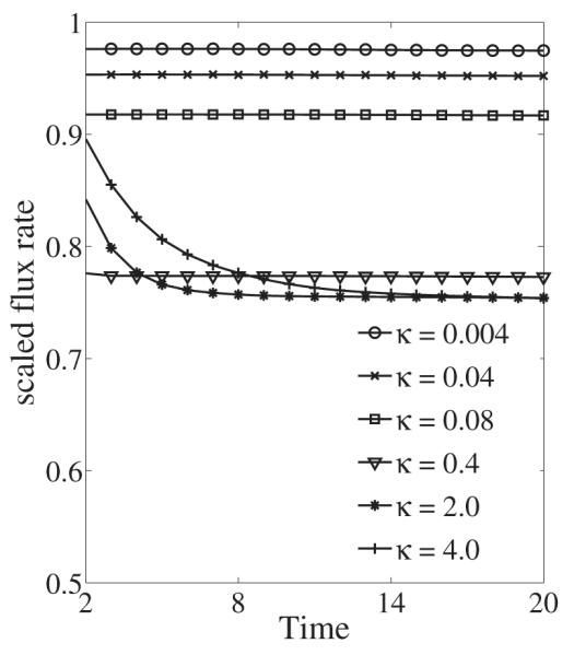
The mean scaled flux for different κ values. The initial network volume-fraction is θⁿ = 0.98 and held fixed in time.

Next, we set the initial network volume-fraction to θⁿ = 0.3 and carry out two sets of simulations that differ only in whether θⁿ is held spatially constant in time or changes according to Eq. (1). As shown in Fig. 8(a), when θⁿ is held spatially constant, the flux is always smaller than that for a single-phase Newtonian fluid and exhibits similar patterns with varying κ as in the previous simulations with θⁿ = 0.98. With less network material in the mixture, there is a smaller reduction in the amount of fluid transport driven by the pump.

Figure 8.

The mean scaled flux for different κ values. (a) Constant θⁿ. (b) Variable θⁿ.

When θⁿ evolved according to Eq. (1), substantial spatial inhomogeneities in θⁿ formed, and a steady flow rate failed to develop. Such strong spatial phase separation is not physical, and stems from the absence in the equations of a term for the chemical interactions between polymers, i.e. swelling stress. Hence, we introduced a chemical pressure Ψ(θⁿ) whose gradient enters on the right hand side of Eq. (4). The specific form of the chemical pressure used is that from Flory-Huggins polymer theory [34]

$$\Psi \left({\theta }^{\mathrm{n}}\right)={\psi }_0\left(\frac{1}{n}{\theta }^{\mathrm{n}}\log \left({\theta }^{\mathrm{n}}\right)+(1-{\theta }^{\mathrm{n}})\log (1-{\theta }^{\mathrm{n}})+\chi {\theta }^{\mathrm{n}}(1-{\theta }^{\mathrm{n}})\right).$$ (28)

The first two terms are entropic terms and the third is an interaction energy term. The parameter n is the number of segments in a polymer chain, χ is the “interaction” parameter whose value is determined from the pairwise interaction energies between two fluid particles, two network particles, or one fluid and one network particle. The amplitude of the chemical pressure is scaled by ψ₀. For this paper, we set n = 1, χ = 2, and ψ₀ = 10, so that the chemical pressure penalizes strong separation of the network and fluid phases. The simulation results with variable θⁿ is plotted in Fig. 8(b). The qualitative relation between the flux and κ remains the same. However, when θⁿ is allowed to vary in space and time, the total flux is higher than the flux for a single-phase Newtonian fluid.

4. Conclusion

We have introduced a new Immersed Boundary method for two-fluid mixtures. In the classic IB method, communication of information between the Lagrangian IB points that represent immersed objects and the fluid (described in Eulerian terms) is done using integral transforms with delta-function kernels. Forces calculated from the configuration of the IB points are transmitted to the surrounding fluid, and the velocity at which each IB point moves is found by interpolating from the velocities at nearby points of that fluid. In extending this idea to a mixture of two fluids, “solvent” and “network”, one is faced with the issue of which force information to communicate to each fluid, and with the issue of deciding at which velocity should IB points move if the fluids have different velocities near the immersed structures. A reasonable boundary condition for many applications is to require that the two fluids have the same velocity at each point on an immersed structure, but, within the usual IB framework, there does not seem to be a mechanism for enforcing this condition. Our way of dealing with these issues is to use two immersed boundaries to represent each immersed structure. Each of these boundaries communicates with only one of the fluids. The force generated within each immersed boundary is transmitted only to the corresponding fluid. The velocity of IB points on each of these boundaries is determined by interpolating velocities from the corresponding fluid. Although the two immersed boundaries representing an immersed structure do not move at exactly the same velocity, their velocities and locations can be made to match closely by defining “penalty” forces between corresponding points of the two boundaries that drive these points together.

One disadvantage of the proposed penalty method is that use of the penalty force imposes an extra restriction on the time step in order for the calculations to remain stable. In the test presented in section 3.1, the tether spring stiffnesses were chosen so that maximum difference between the IB point locations and their target locations was less than 0.02∊, where ∊ is the amplitude of the wave. For a single-phase fluid, the stiffness of the tether springs limited the time step to a Courant number of about 0.1. For the two-fluid case, the stiffness of the penalty spring was selected so that the distance between the two IB boundaries remained below 0.05h, where h is the size of the computational grid. The maximum stable time step in these tests corresponded to a Courant number of 0.02, which is five times smaller than the maximum size step that produced stable calculations when the method was applied to a single-phase fluid.

An alternative approach to our penalty method, which might allow a larger time step, is a constraint-based approach in which constraint forces are determined to ensure that the two fluids have the same velocity on each of the immersed boundaries [35, 36, 37], an approach which we have found effective in another context [38]. While exploration of these approaches for the current problem is warranted, their application here is not straightforward. One issue is that we are solving multi-fluid analogs of time-independent Stokes equations, and the methods in [37] are based on a fractional-step treatment of the Navier-Stokes equations. Another complication is that our momentum equations involve time and space dependent coefficients, so that preprocessing of the matrices involved in their solution is not an option.

We have applied the new method to three problems all involving interactions of one or more immersed structures with two viscous fluids or with a viscous fluid and a viscoelastic one. For the first two problems, we solved the momentum and incompressibility equations and the volume-fraction evolution equation using the methods described in [33]. The first problem is the two-fluid version of G.I. Taylor’s swimming sheet problem in which an imposed undulating motion of a sheet results in a net translational motion of the sheet. Using this as a test problem, we demonstrated that the new method converges and has approximately first-order accuracy, similar to the classic IB method for a single fluid. We also explored the effect of the ratio of the two fluids’ viscosities and the composition of the mixture on the sheet’s swimming speed.

The second problem involves peristaltic pumping of a two-fluid mixture. We confirmed that in the case that we set the two fluid’s viscosities equal and began with a spatially-uniform volume-fraction distribution, the new method produced results in agreement with existing theories for peristalsis of a single fluid. We then applied the method to peristalsis of a two-fluid mixture and saw that for a given motion of the tube walls, the total flux in the case of two fluids with different viscosities exceeds that for a single fluid of either viscosity. We carried out simulations of peristalsis in which particles were added to the two-fluid mixture. The presence of the particles substantially altered the relative motion of the two fluids and led to more pronounced volume-fraction heterogeneities than we observed without particles. The particle simulations also showed that our new method is able to handle objects whose motion is “free” and determined only by their interactions with the surrounding fluids. Also these simulations demonstrated that the calculated behavior of the fluids inside the peristaltic tubes was affected little by the conditions outside of the tube. To our knowledge, this is the first time that independence of external conditions has been demonstrated in using Immersed Boundary methods to study complex fluids.

The third problem we investigated with the new method again involved peristalsis, but this time the network was modeled as an Oldroyd-B viscoelastic fluid. For this problem, we solved the momentum and incompressibility equations and the volume-fraction, elastic-link density, and viscoelastic-stress evolution equations using the methods described in [24]. The influence of viscoelasticity was to reduce the flux driven by the peristaltic motion, an observation consistent with that by Teran et al [11] for a single Oldroyd-B fluid. In the two-fluid case, there is competition between the flux-reducing effect of the viscoelasticity and the flux-increasing effect of the relative motion and phase separation of the mixture. Thus for some parameter regimes the net flux was higher than for a single fluid, while for others it was lower. Further investigation of this competition is ongoing.

References

- [1].Peskin CS. The Immersed Boundary Method. Acta Numerica. 2002;11:479–517. [Google Scholar]
- [2].McQueen DM, Peskin CS. Computer-assisted design of pivoting disc prosthetic valves. J. Thorac. Cardiovasc. Surg. 1983;86:126. [PubMed] [Google Scholar]
- [3].McQueen DM, Peskin CS. Shared-memory parallel vector implementation of the immersed boundary method for the computation of blood flow in the beating mammalian heart. J. Supercomputing. 1997;11:213–236. [Google Scholar]
- [4].Griffith BE, Luo X, McQueen DM, Peskin CS. Simulating the fluid dynamics of natural and prosthetic heart valves using the immersed boundary method. Int. J. Appl. Mech. 2009;1:137–177. [Google Scholar]
- [5].Fogelson AL. A mathematical model and numerical method for studying platelet adhesion and aggregation during blood clotting. J. Comput. Phys. 1984;56:111–134. [Google Scholar]
- [6].Fogelson AL, Guy RD. Immersed-boundary-type models of intravascular platelet aggregation. Comput. Method Appl. Mech. Eng. 2008;(197):2087–2104. [Google Scholar]
- [7].Fauci LJ, Peskin CS. A computational model of aquatic animal locomotion. J. Comput. Phys. 1988;77:85–108. [Google Scholar]
- [8].Fauci LJ, McDonald A. Sperm motility in the presence of boundaries. B. Math. Biol. 1994;57:679–699. doi: 10.1007/BF02461846. [DOI] [PubMed] [Google Scholar]
- [9].Tytell E, Hsu C, Williams T, Cohen A, Fauci L. Interactions between internal forces, body stiffness, and fluid environment in a neuromechanical model of lamprey swimming. Proc. National Acad. of Sciences. 2010;107:19832–19837. doi: 10.1073/pnas.1011564107. [DOI] [PMC free article] [PubMed] [Google Scholar]
- [10].Bottino DC. Modeling viscoelastic networks and cell deformation in the context of the immersed boundary method. J. Comput. Phys. 1998;147:86–113. [Google Scholar]
- [11].Teran J, Fauci L, Shelley M. Peristaltic pumping and irreversibility of a Stokesian viscoelastic fluid. Phys. Fluids. 2008;20:073–101. [Google Scholar]
- [12].Chrispell J, Fauci L. Peristaltic pumping of solid particles immersed in a viscoelastic fluid. Math. Model. Nat. Phenom. 2011;6:67–83. [Google Scholar]
- [13].Miller LA, Peskin CS. When vortices stick: an aerodynamic transition in tiny insect flight. J. Exp. Biol. 2004;207:3073–3088. doi: 10.1242/jeb.01138. [DOI] [PubMed] [Google Scholar]
- [14].Miller LA, Peskin CS. Flexible clap and fling in tiny insect flight. J. Exp. Biol. 2009;212:3076–3090. doi: 10.1242/jeb.028662. [DOI] [PubMed] [Google Scholar]
- [15].Dillon R, Fauci LJ, Fogelson AL, Gaver D. Modeling biofilm processes using the immersed boundary method. J. Comput. Phys. 1996;129:57–73. [Google Scholar]
- [16].Grunbaum D, Eyre D, Fogelson AL. Functional geometry of ciliated tentacular arrays in active suspension feeders. J. Exp. Biol. 1998;201:2575–2589. doi: 10.1242/jeb.201.18.2575. [DOI] [PubMed] [Google Scholar]
- [17].Musielak M, Karp-Boss L, Jumars P, Fauci L. Nutrient transport and acquisition by diatom chains in a moving fluid. J. Fluid Mech. 2009;638:401–421. [Google Scholar]
- [18].Hamlet C, Santhanakrishnan A, Miller LA. A numerical study of the effects of bell pulsation dynamics and oral arms on the exchange currents generated by the upside-down jellyfish Cassiopea spp. J. Exp. Biol. 2011;214:1911–1921. doi: 10.1242/jeb.052506. [DOI] [PubMed] [Google Scholar]
- [19].Bhalla A, Bale R, Gridth BE, Patankar NA. Fully resolved immersed electrohy-drodynamics for particle motion, electrolocation, and self-propulsion. J. Comput. Phys. 2014;256:88–108. [Google Scholar]
- [20].Jubery TZ, Dutta P. A fast algorithm to predict cell trajectories in microdevices using dielectrophoresis. Numer. Heat Tran. A. 2013;64:107–131. [Google Scholar]
- [21].Kandilarov JD, Vulkov LG. Analysis of immersed interface difference schemes for reaction-diffusion problems with singular own sources. Comput. Methods Appl. Math. 2003;3:253–273. [Google Scholar]
- [22].Bhalla A, Gridth BE, Patankar NA, Donev A. An immersed boundary method for reaction-diffusion problems. 2013. arXiv preprint arXiv:1306.3159. [DOI] [PubMed]
- [23].Fu HC, Shenoy VB, Powers TR. Low-Reynolds-number swimming in gels. Europhys. Lett. 2010;91:24002. [Google Scholar]
- [24].Wright GB, Guy RD, Du J, Fogelson AL. A high-resolution finitedifference method for simulating two-fluid, viscoelastic gel dynamics. J. Non-Newtonian Fluid Mech. 2011;166:1137–1157. [Google Scholar]
- [25].Tu C, Peskin CS. Stability and Instability in the Computational of Flows with Moving Immersed Boundaries: A Comparison of Three Methods. SIAM J. Sci. Stat. Comput. 1992;13:1361–1376. [Google Scholar]
- [26].Fauci LJ, Fogelson AL. Truncated Newton Methods and the Modeling of Complex Immersed Elastic Structures. Comm. Pure Appl. Math. 1993;46:787–818. [Google Scholar]
- [27].Colella P. Multidimensional upwind methods for hyperbolic conservation laws. J. Comput. Phys. 1990;87:171–200. [Google Scholar]
- [28].Taylor GI. Analysis of the swimming of microscopic organisms. Proc. R. Soc. A. 1951;209:447–461. [Google Scholar]
- [29].Reynolds AJ. The swimming of minute organisms. J. Fluid Mech. 1965;23:241–260. [Google Scholar]
- [30].Lauga E. Propulsion in a viscoelastic fluid. Phys. Fluids. 2007;19:083104. [Google Scholar]
- [31].Du J, Keener JP, Guy RD, Fogelson AL. Low Reynolds-number swimming in viscous two-phase fluids. Phy. Rev. E. 2012;85:036304. doi: 10.1103/PhysRevE.85.036304. [DOI] [PubMed] [Google Scholar]
- [32].Jaffrin M, Shapiro A. Peristaltic pumping. Annu. Rev. Fluid Mech. 1971;3:13–37. [Google Scholar]
- [33].Wright GB, Guy RD, Fogelson AL. An efficient and robust method for simulating two-phase gel dynamics. SIAM J. Sci. Comput. 2008;30:2535–2565. [Google Scholar]
- [34].Doi M, See H. Introduction to Polymer Physics. Oxford University Press; 1996. [Google Scholar]
- [35].Uhlmann M. First experiments with simulation of particulate flows. Technical reports. 2003;1020 issn: 1135-9420. [Google Scholar]
- [36].Bhalla A, Bale R, Gridth BE, Patankar NA. A unified mathematical framework and an adaptive numerical method for fluid-structure interaction with rigid, deforming, and elastic bodies. J. Comput. Phys. 2013;250:446–476. [Google Scholar]
- [37].Taira K, Colonius T. The immersed boundary method: a projection approach. J Comput Phys. 2007;225:2118–2137. [Google Scholar]
- [38].Yao L, Fogelson AL. Simulations of chemical transport and reaction in a suspension of cells I: an augmented forcing point method for the stationary case. Int. J. Numer. Meth. Fluids. 2012;69:1736–1752. [Google Scholar]