A framework for multi-scale modelling

Abstract

We review a methodology to design, implement and execute multi-scale and multi-science numerical simulations. We identify important ingredients of multi-scale modelling and give a precise definition of them. Our framework assumes that a multi-scale model can be formulated in terms of a collection of coupled single-scale submodels. With concepts such as the scale separation map, the generic submodel execution loop (SEL) and the coupling templates, one can define a multi-scale modelling language which is a bridge between the application design and the computer implementation. Our approach has been successfully applied to an increasing number of applications from different fields of science and technology.

1. Introduction

Multi-scale models and simulations are an important challenge for computational science in many domains of research. Most real-life phenomena involve an extended range of spatial or temporal scales, as well as the interaction between various natural processes. When these interacting processes are modelled by different scientific disciplines, they are multi-science (or multi-physics) as well as multi-scale. Biomedical applications, where biology is coupled to fluid mechanics, are an illustration of a multi-scale, multi-science problem. For instance, in the problem of in-stent restenosis [1–4], blood flow, modelled as a purely physical process, is coupled to the growth of smooth muscle cells (SMCs). Haemodynamics is a fast varying process, acting over spatial scales ranging from micrometres to centimetres. On the other hand, SMCs evolve at a much slower time scale of days to weeks.

Although the term ‘multi-scale modelling’ is commonly used in many research fields, there are only a few methodological papers [5–8] offering a conceptual framework, or a general theoretical approach. As a result, in most of the multi-scale applications found in the literature, methodology is entangled with the specificity of the problem and researchers keep reinventing similar strategies under different names. A more developed discussion of the status of multi-scale modelling in various scientific communities is presented in this Theme Issue [9].

It is clear that a well-established methodology is quite important when developing an interdisciplinary application within a group of researchers with different scientific backgrounds and different geographical locations. A multi-scale modelling framework and a corresponding modelling language is an important step in this direction. It allows one to clearly describe multi-scale, multi-science phenomena, separating the problem-specific components from the strategy used to deal with a large range of scales.

From a practical aspect, many codebases for single-scale models already exist. Using a component-based approach is a way to re-use these existing models and codebases. A modelling language is used to make a blueprint of a complex application, offering a way to co-develop a global numerical solution within a large team. A good match between the application design and its implementation on a computer is central for incremental development and its long-term sustainability.

In this paper, we will review the so-called Multiscale Modelling and Simulation Framework (MMSF) that we have been developing over the past few years within the European projects COAST (http://www.complex-automata.org) and MAPPER (http://www.mapper-project.eu). This framework is a step towards a solution to the problems identified above. Its main emphasis is in pressing multi-scale modellers to clearly separate single-scale models and the scale bridging methods needed for them to interact. Within the MAPPER project (http://www.mapper-project.eu), MMSF has been applied and evaluated on seven different applications. These applications are described in more detail in another contribution in this Theme Issue [10].

2. The Multiscale Modelling and Simulation Framework

The MMSF is a theoretical and practical way to model, describe and simulate multi-scale, multi-science phenomena. By adhering to a single framework, not tied to a specific discipline, groups of researchers ensure that their respective contributions may cooperate with those of others. MMSF is described in detail in [11] and references therein. Here, we review the main ideas of the formalism.

Figure 1 summarizes the entire pipeline implementing MMSF. It reflects the fact that developing a multi-scale application requires several steps. First, we have to model the phenomena we want to study by identifying the relevant scales and the relevant processes (submodels) that are involved. In this framework, we assume that submodels have at least a temporal and spatial scale and focus on those, but other scales may be used in their place. Once the components and their scale have been identified, we have to indicate how they are coupled and which scale bridging techniques are required. This second step is aided by the Multiscale Modelling Language (MML) [11,12], which describes the architecture of a multi-scale model. It describes the scales and computational requirements of submodels and scale bridging components, each with predefined output and input ports used for communicating data. These ports are associated with a datatype and a communication rate tied to the submodel scales, and an output port can be coupled to an input port if these data types and rates match.

Figure 1.

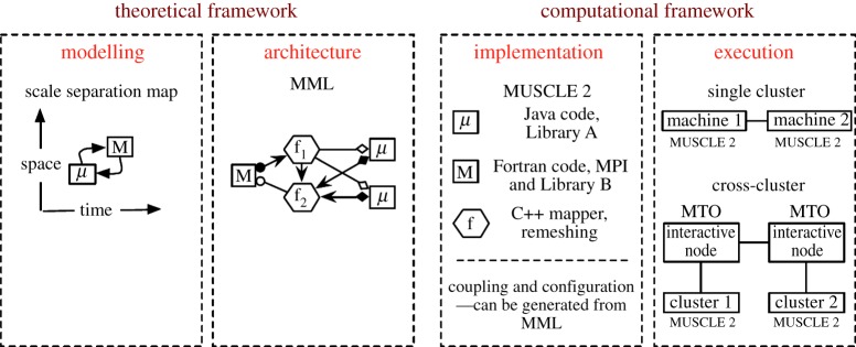
The pipeline of actions needed to develop and run a multi-scale application within MMSF. (Online version in colour.)

The third step concerns the implementation of the single-scale models (or the reuse of existing ones), and the implementation of scale bridging techniques. Existing single-scale model codes will require small changes to enable coupling with other models, while scale bridging techniques will need to be implemented specifically for the single-scale models that they are coupled to, in the form of so-called filters or mappers (see below for a definition). The software MUSCLE 2 [13,14] follows this paradigm. To use single-scale model code with MUSCLE 2, simply insert send and receive calls to local output and input ports. These ports are coupled separately from the submodel implementation, in MML, so that submodels do not have to know what code they are coupled to. MUSCLE 2 can couple submodels written in different programming languages, e.g. Fortran with C++, or a massively parallel MPI code with a multi-thread Java program.

Finally, in the fourth step of the pipeline shown in figure 1, the different submodels are executed on a computing infrastructure. In our approach, they can be distributed on different computers, without extra software development. This is called distributed multi-scale computing (DMC) [10,15]. It is made possible by the runtime environment of MUSCLE 2, which can exchange data between computers, whether remote or not.

Steps 3 and 4 above relate to the computational framework. They are described in [14] and will not be discussed further here. However, a performance study of DMC can be found in another contribution in this Theme Issue [10]. In what follows we focus on the conceptual and theoretical ideas of the framework.

(a). The scale separation map

A multi-scale system can be represented on a scale separation map (SSM), i.e. a map that describes the range of spatial and temporal scales that need to be resolved in order to solve the problem at hand. This range of scales is shown as a rectangle, as indicated in figure 2a. In order to simulate such a process on a computer, one has to find a strategy to ‘split’ these scales and keep only the relevant ones. One aspect of this is choosing which physics to model. Otherwise, a high computational cost will result, together with an explosion of data and only limited knowledge. This process amounts to the identification of submodels acting on a reduced range of scales, and their mutual couplings, as illustrated in figure 2b. Each of these submodels may require different computing resources. Some may be massively parallel, others may require special hardware and software, and may run optimally on a different number of cores. This is illustrated in figure 2c. This figure also shows that the computing resources may exhibit a ‘multi-scale parallelism’ as the number of cores associated with each submodel may vary across several orders of magnitude. Thus, the term DMC refers both to the multi-scale nature of the application and to the computing infrastructure. Note, however, that the degree of parallelism may not scale with the physical scales. Parallelism may actually be higher for coarse-scale models. For example, in the nano-materials application described in [10], 64 cores are used for the atomistic scale, whereas 1024 are used for the molecular scales.

Figure 2.

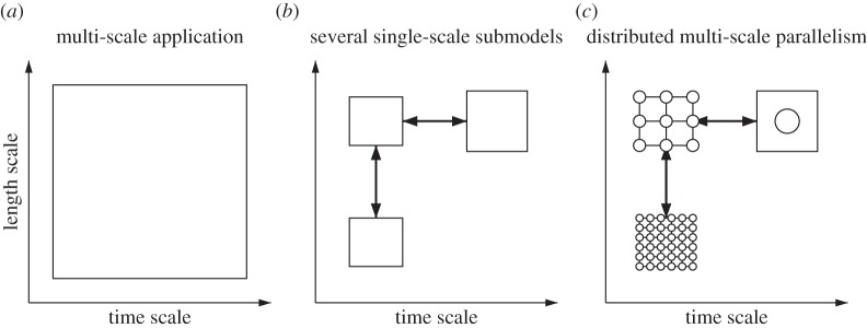
Illustration of the process of ‘scale splitting’: a multi-scale model (a) is decomposed into several ‘single-scale’ coupled submodels (b). Finally, the application is executed on a computing infrastructure with multi-scale degrees of parallelism (c).

Note that the SSM can give a quick estimate of the CPU time gained by the scale splitting process when it concerns a mesh-based calculation. The CPU time of a submodel goes as (L/Δx)^d(T/Δt), where d is the spatial dimension of the model, and (Δx,L) and (Δt,T) are the lower-left and upper-right coordinates of the rectangle shown on the SSM. Therefore, the computational time of the system in figure 2a is likely to be much larger than those in figure 2b.

The splitting of a problem into several submodels with a reduced range of scales is a difficult task which requires a good knowledge of the whole system. This separation of scales is likely to affect the quality of the result, when compared with a fully resolved (yet unaffordable) computation. The art of multi-scale modelling is then to propose a good compromise between CPU performance and accuracy by selecting the most relevant parts of the domain at an appropriate scale. Finding a proper accuracy metrics and the right balance between precision and CPU requirements is a wide open question [9]. We believe that MMSF will contribute to exploring these highly relevant issues. An early example is the work we did on finding multi-scale modelling errors in a reaction–diffusion model [16].

The arrows shown in figure 2 represent the coupling between the submodels that arise due to the splitting of the scales. They correspond to an exchange of data, often supplemented by a transformation to match the difference of scales at both extremities. They implement some scale bridging techniques that depend on the nature of the submodels and the degree of separation of the scales.

In our methodology, these couplings are implemented as software components, coined smart conduits that completely take care of the mapping of the data from one submodel to the other. Therefore, in the MMSF approach, submodels are autonomous solvers that are not aware of the scales of the other submodels and that can be substituted any time by a better version of the code or the algorithm. The smart conduits, which are scale-aware, are of three types: plain conduits, filters and mappers. Plain conduits simply transfer messages, whereas filters modify in-transit messages, according to the scales of the submodels they connect. Mappers may combine inputs from multiple conduits and produce multiple outputs. Combined, these constructs are used for implementing scale bridging methods, but they are not part of the scale separation map since they are not part of the single-scale models. These constructs are explicitly described in §3. This section includes more information on the multi-scale model architecture and discusses the MML.

The relation between two submodels can be described through their respective positions on the SSM. Here, we consider only two axes, space and time, but in general the SSM can include any relevant dimensions. In the SSM, the scales of the two submodels either overlap or can be separated. When scale-overlap or scale-separation concerns two quantities, there are five possible relations in total, as illustrated in figure 3.

Figure 3.

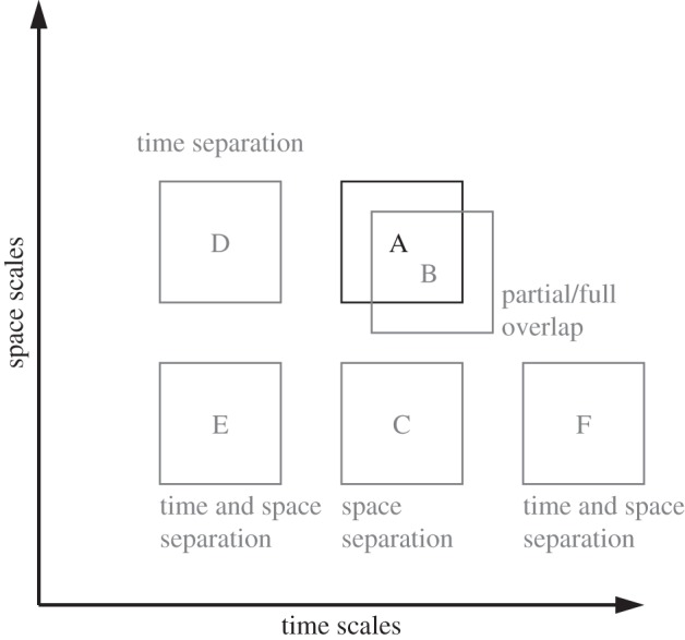
The five possible relations between two submodels in the SSM. Model A is the reference submodel. Submodel B corresponds to a scale overlap situation. Then, with submodels C, D, E and F, we illustrate scale separation either in time or in space, or both.

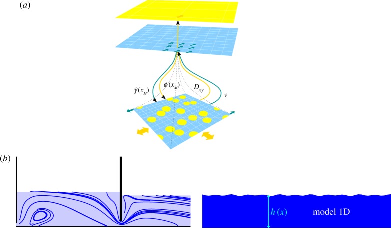
In addition to their respective positions on the SSM, two interacting submodels are characterized by the relation between their computational domains. Both submodels can share the same domain, a situation termed sD for single domain. Otherwise, the submodels have different or slightly overlapping computational domains. This case is termed mD for multi-domain. Figure 4 illustrates the two situations in a specific case. Figure 4a shows a fluid with suspensions. At the coarser scale, the system is solved by coupling the Navier–Stokes equations with an advection–diffusion model for the suspension. The viscosity and diffusion coefficients can be computed from a fully resolved simulation, at a smaller scale, for each shear rate condition [17]. Figure 4b shows a free surface flow model describing the flow under a gate, coupled with a low-resolution shallow water model describing the downstream flow. A very small overlap between the two sub-domains may be needed to implement the coupling.

Figure 4.

Relation between the computational domains of two submodels. (a) The two submodels share the same domain, but at different scales. This situation is called single domain (sD). (b) The full computational domain is distributed over two submodels, with possibly an overlap for coupling them. This situation is called multi-domain (mD). (Online version in colour.)

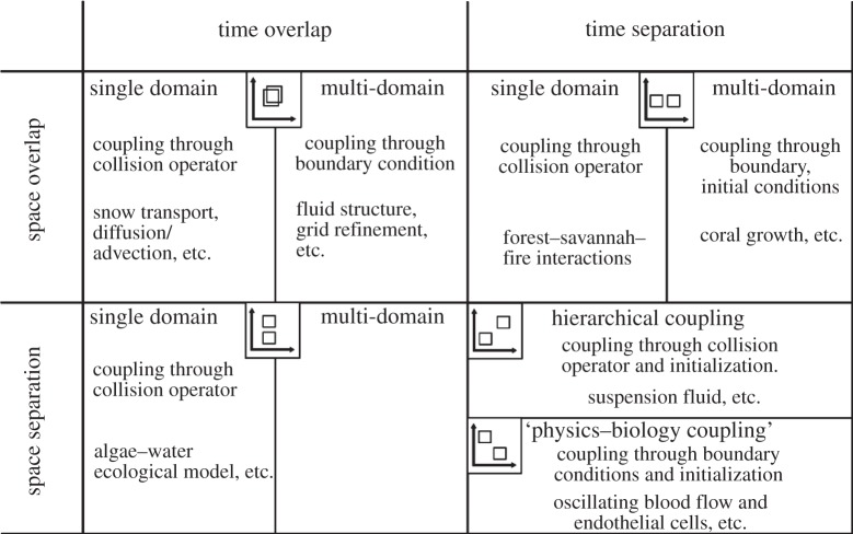
The above features (respective position in the SSM and domain relation) offer a way to classify the interactions between two coupled submodels. Figure 5 summarizes this classification in several regions. An indication of the type of coupling is given. We refer the reader to the next section for an explanation.

Figure 5.

A classification of multi-scale problems, based on the separation of the submodels in the SSM, and based on the relation between their computational domain (see [18] for more details). As discussed in the next section, only a few couplings seem to occur in these examples.

In figure 5, examples are also mentioned. We will elaborate on two of them. The forest–savannah–fire example uses cellular automata to model grasslands that evolve into forests which are occasionally affected by forest fires [19]. The model takes a grid as the domain. Grid points with small herbs are gradually converted to pioneering plants and finally into forest, with a time scale of years. A forest fire, on the other hand, may start and stop within a day or a few weeks at the most. If these two processes are decomposed, a vegetation submodel could take a grid with the vegetation per point and a fire submodel only needs a grid with points marked as able to burn or not. Clearly, the underlying domain overlaps, making it a single-domain problem. Conceptually, the vegetation submodel could send its domain at each iteration, the forest fire submodel may decide to start a fire, and return a list or grid of points that were burnt down. The vegetation submodel keeps running, while the forest fire submodel is restarted at each iteration. Practically, the two submodels might modify a shared data structure. However, the runtime environment will determine whether this is actually possible, or if they have to modify separate data structures which are combined after each iteration (see figure 6 for a number of execution options). The latter option is necessary if the submodels are executed on different machines, or if the forest fire and vegetation submodels use different resolutions. If they have different resolutions, a mapper may run between the vegetation and forest fire submodel to map a grid of one resolution to another. Alternatively, multiple vegetation submodels might be run concurrently, and a single forest fire submodel might run on the combined domain. The vegetation submodels would have mD interactions, exchanging only boundary information, but they would have sD interactions with the fire submodel. A mapper would be placed between the vegetation and forest fire submodels to stitch the grids of the vegetation submodels together, so that it would not have to be aware whether the vegetation is simulated by a single or by multiple domains. In this scenario, the vegetation submodels must be designed to allow boundary interaction, but they may be simulated in isolation by letting a mapper provide specially made boundary data. There is probably a performance benefit to using a single data structure, but separating the submodels provides more clarity and provides a path to directing parallelization efforts towards only parts of a code.

Figure 6.

Runtime options for the forest–savannah–fire model. On the left, a single data structure is used for simulating fire and vegetation; in the middle separate data structures are used; and on the right, the vegetation is decomposed into multiple domains, where the fan-in and fan-out mappers make the right conversion between the domains. The middle- and right-hand-side figures may be run with largely the same code. (Online version in colour.)

The second application we briefly discuss here is the suspension fluid example. It is characterized by temporal and spatial scale separation. A hard sphere suspension model is used on the fine scale, an advection–diffusion model on the meso-scale, and a non-Newtonian fluid dynamics model on the coarse-scale [20]. The fine-scale model is needed to get accurate dynamics, whereas the coarse-scale model is able to simulate large domains. The scale bridging between the scales is far from trivial and determines how well the coarse-scale simulation eventually describes the system. It relies on simulating many fine-scale suspensions at each coarse-scale time step. A mapper is in charge of a strategy to simulate the submodels, so the coarse-scale model may simply provide and retrieve values at its grid points.

To further illustrate the fact that the SSM is a powerful way to describe a multi-scale, multi-science problem, let us consider the SSM corresponding to a real problem with more than two submodels. Figure 7 describes the case of in-stent restenosis [1,4,21]. After the stenting of a coronary artery, the SMCs are likely to proliferate into the lumen, causing again a stenosis. Drug-eluting stents can be used to slow down the SMC growth. Note that, here, the couplings have been annotated with the quantities that are exchanged between each pair of submodels. The scale bridging will take place in the coupling, and this will be described by the multi-scale modelling language.

Figure 7.

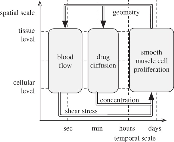
SSM of the in-stent restenosis application described in [1,21].

From this picture we see that, contrary to many situations reported in the literature, multi-scale modelling is more than the coupling of just two submodels, one at a microscopic scale and the other at a macroscopic scale.

(b). Submodel execution loop and coupling templates

A second ingredient of the MMSF methodology is to express the models with a generic, abstract execution temporal loop. We term this algorithmic structure the SEL. It reflects the fact that, during the time iterations of the submodels, a reduced set of generic operations have to be performed over and over again. The most important one is the S operation, where S refers to Solver. A second important step of the SEL is the B operation, where B means Boundary. The execution of B amounts to specifying the boundary conditions for the computation. The repetition of S and B is the core of the submodel time loop. Separating S and B is conceptually useful but if separation is not possible or practical, all functionality can be incorporated in the S operation directly. In each iteration of the loop, the simulated time is increased based on the temporal scale of the submodel. Operations that are finer than this temporal scale and operations that are not time dependent may be placed inside the S or B operations instead of being represented explicitly in the SEL.

In addition, in order to initialize the process, another operation has to be specified. In our approach, we term it f_init to reflect that the variables of the model need to be given an initial value. This initialization phase also specifies the computational domain and possibly some termination condition for the time loop.

Finally, we define two observation operators, O_i and O_f, which compute some desired quantities from the model variables. The subscript i and f are for intermediate and final observations, respectively.

Imposing the above generic structure on the evolution loop limits the ways to couple two submodels. A coupling amounts to an exchange of data between a pair of operators belonging to the SEL of the two submodels. According to our definitions, the sender of information is either O_i or O_f. And the receiving operators can only be S, B or f_init. This is illustrated in figure 8.

Figure 8.

The generic SEL and two examples of coupling templates.

We call coupling templates the different possible pairs of input/output operators in a coupling. Therefore, the coupling templates are O_i→S, O_i→B, O_i→f_init and O_f→S, O_f→B, O_f→f_init. These coupling templates can be named as in table 1.

Table 1.

Relation between coupling templates and position in the SSM for two submodels X and Y sharing the same computational domain.

name	coupling	temporal scale relation
interact	OXi→SY	overlap
call		X larger than Y
release	OYf→SX	Y smaller than X
dispatch		any

It is quite interesting to note that these coupling templates reflect very closely the relative position of the two submodels in the SSM and the relation between their computational domains. From analysing several multi-scale systems and the way their submodels are mutually coupled, we reach the conclusion that the relations shown in table 1 hold between any two coupled submodels X and Y with a single-domain relation. In cases where X and Y have a multi-domain relation, the same table holds but the operator S is replaced by B.

To illustrate the meaning of table 1, we can consider a system of particles transported in a fluid flow. Submodel X is the fluid solver and submodel Y is an advection–diffusion solver. This is a typical single-domain situation with overlapping temporal scales. The observation O^X_i of the flow velocity is needed to compute the advection process. So O^Y_i→S^X. In return, O^X_i→S^Y because the density of transported particles may affect the viscosity of the fluid.

In the example of the growth of biological cells subjected to the blood flow shear stress, there is a clear time-scale separation between the two processes (see figure 7 and [22]). Therefore, the converged flow field is first sent from the physical model BF to the biological one, in order to define the SMC proliferation rate in SMC (O^BF_f→S^SMC). Then, the new geometry of the cells induces a new boundary condition for the flow, which must be recomputed ().

3. Multiscale Modelling Language

The underlying execution model assumed for MMSF is typically data-driven. Submodels run independently, requiring and producing messages at a scale-dependent rate. A message contains data on the submodel state, the simulation time that the data were obtained, and the time that the submodel will send the next message, if any.

Figure 9 describes typical workflows that couple submodels. Depending on the detail of the model, the interaction between two submodels may have feedback or not, signified by a one- or two-way coupling. In general, the coupling topology of the submodels may be cyclic or acyclic. In acyclic coupling topologies, each submodel is started once and thus has a single synchronization point, while in cyclic coupling topologies, submodels may get new inputs a number of times, equating to multiple synchronization points. The number of synchronization points may be known in advance (static), in which case they may be scheduled, or the number may depend on the dynamics of the submodels (dynamic), in which case the number of synchronization points will be known only at runtime. Likewise, the number of submodel instances may be known in advance (single or static) or be determined at runtime (dynamic). This last option means a runtime environment will need to instantiate, couple and execute submodels based on runtime information.

Figure 9.

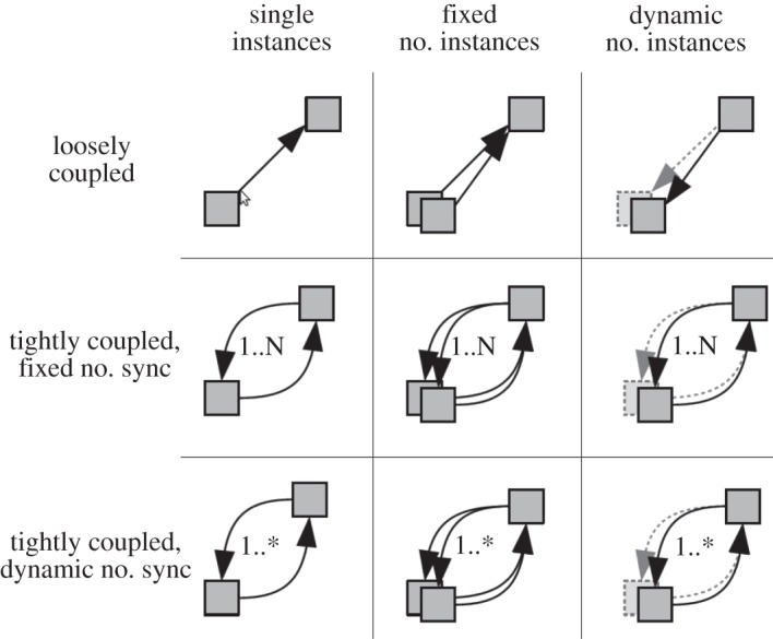
The different workflows identified in our framework, and corresponding to the coupling of two submodels.

The language is part of MMSF and provides a formalization of the concepts introduced previously. In addition to describing the coupling architecture of a multi-scale model, it also contains information about its computational requirements. This information does not impose a unique implementation, but rather forms a specification of what behaviour should be expected from each element of the system. A submodel may be described as having a number of inputs and outputs at given SEL operators, and be associated with an executable to run the simulation of that submodel. MML does not specify what algorithms are computed in a submodel, nor what their implementation will be, but it can describe its functionality and computational details like parallelism, programming language and memory requirements.

The components of MML are depicted graphically in figure 10. MML can also be expressed as an XML file [11,12] for automatic processing. This file format contains additional meta-data about the submodels and their couplings. They represent the data transfer channels that couple submodels together. Conduits implement one-way, point-to-point communications. Filters are state-full conduits, performing data transformation (e.g. scale bridging operations). Finally, mappers are multi-port data-transformation devices.

Figure 10.

The components of MML in a graphical form. Conduits are shown on the left and mappers on the right.

Mappers are useful to optimize a coupling, for instance to avoid repeating twice the same data transformation for two different recipients. They are also needed to build complex couplings, and to implement synchronization operations when more than two submodels are coupled. The fan-in and fan-out mappers, whose behaviour is explained in figure 10, are sufficient to model complex situations. The output of a mapper is produced when all inputs are present.

As shown in figure 10, the extremities of conduits carry some symbols. These symbols indicate which coupling template they correspond to, or which operator of the SEL they have for source or for destination. The XML file format contains information about the data type and contents of couplings, while the operators in the SEL and the conduits implement the proper algorithms.

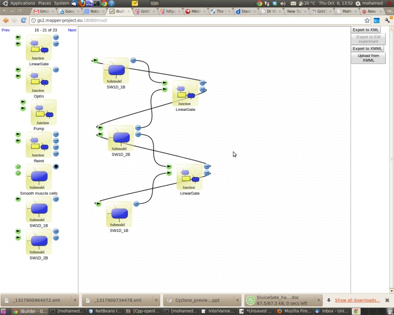
In MMSF, submodels, filters and mappers can be parametrized and stored in a repository to be re-used for other applications. A tool [15,23] is available to compose new applications by a drag and drop operation, using previously defined components. This is illustrated in figure 11.

Figure 11.

The Lego-based approach made possible by MML and the MAD tool. Predefined software components (submodels, filters and mappers) visible on the left-hand side of the screen can be moved to the design window and connected through their input and output ports. These ports corresponds to the SEL operators and are represented with different symbols and colours. (Online version in colour.)

Finally, figure 12 shows the full MML diagram corresponding to the application described in figure 7.

Figure 12.

The MML description of the in-stent restenosis model (see also figure 7). Here, BF stand for the blood flow submodel, SMC for the biological growth of smooth muscle cells, DD for drug diffusion and IC for injury score (the initial condition).

4. Conclusion

In this paper, we have formalized the process of multi-scale modelling and simulation in terms of several well-defined steps. This formalization is important in order to give precise definitions of the concepts and to disentangle implementation issues from the modelling ones.

Our MMSF approach contains several distinguishing and original features. It is not linked to a specific application domain. It is based on new generic theoretical concepts describing the entire process, from design to execution. It facilitates the communication between scientists of different fields, provides a unified vision of multi-scale modelling and simulation, and offers a common framework for consistent new developments. Beyond its methodological contents, MMSF is operational and supported by a full implementation and execution framework, based on MUSCLE 2 and the idea of DMC and multi-scale parallelism. The MUSCLE 2 middleware offers a powerful, flexible and easy way to couple new or legacy submodels, independently of the programming language used to code them.

Focusing on the splitting and single-scale models gives the benefit of using proven models (and code) for each part of a multi-scale model. It allows the user to build a multi-scale application referring to the existing theoretical knowledge about the phenomena at each identified scale.

The full approach has been applied successfully within the MAPPER project to design and/or implement and run seven applications belonging to various fields of engineering and science (see [10] for a description). The experience with applying the MMSF to these applications is that it saved a lot of development time, was portable (in terms of both software and hardware), allowed new challenging problems to be addressed, and let users concentrate their efforts on science rather than on implementation issues. Compartmentalizing a model as proposed in MMSF means having fewer within-code dependencies, thereby reducing the code complexity and increasing its flexibility.

Funding statement

The research presented in this contribution is partially supported by the MAPPER project, which receives funding from the EU's Seventh Framework Programme (FP7/2007-2013) under grant agreement no. RI-261507.

References

- 1.Evans D, et al. 2008. The application of multi-scale modelling to the process of development and prevention of stenosis in a stented coronary artery. Phil. Trans. R. Soc. A 366, 3343–3360. ( 10.1098/rsta.2008.0081) [DOI] [PubMed] [Google Scholar]
- 2.Tahir H, Hoekstra AG, Lorenz E, Lawford PV, Hose DR, Gunn J, Evans DJW. 2011. Multi-scale simulations of the dynamics of in-stent restenosis: impact of stent deployment and design. Interface Focus 1, 365–367. ( 10.1098/rsfs.2010.0024) [DOI] [PMC free article] [PubMed] [Google Scholar]
- 3.Tahir H, Bona Casas C, Hoekstra AG. 2013. Modelling the effect of a functional endothelium on the development of in-stent restenosis. PLoS ONE 8, 66138 ( 10.1371/journal.pone.0066138) [DOI] [PMC free article] [PubMed] [Google Scholar]
- 4.Groen D, et al. 2013. Flexible composition and execution of high performance, high fidelity multiscale biomedical simulations. Interface Focus 3, 20120087 ( 10.1098/rsfs.2012.0087) [DOI] [PMC free article] [PubMed] [Google Scholar]
- 5.Weinan E, Li X, Ren W, Vanden-Eijnden E. 2007. Heterogeneous multiscale methods: a review. Commun. Comput. Phys. 2, 367–450. [Google Scholar]
- 6.Ingram GD, Cameron IT, Hangos KM. 2004. Classification and analysis of integrating frameworks in multiscale modelling. Chem. Eng. Sci. 59, 2171–2187. ( 10.1016/j.ces.2004.02.010) [DOI] [Google Scholar]
- 7.Dada JO, Mendes P. 2011. Multi-scale modelling and simulation in systems biology. Integr. Biol. 3, 86–96. ( 10.1039/c0ib00075b) [DOI] [PubMed] [Google Scholar]
- 8.Yang A, Marquardt W. 2009. An ontological conceptualizatin of multiscale models. Comput. Chem. Eng. 33, 822–837. ( 10.1016/j.compchemeng.2008.11.015) [DOI] [Google Scholar]
- 9.Hoekstra A, Chopard B, Coveney P. 2014. Multi-scale modelling and simulation: a position paper. Phil. Trans. R. Soc. A 372, 20130377 ( 10.1098/rsta.2013.0377) [DOI] [PubMed] [Google Scholar]
- 10.Borgdorff J, et al. 2014. Performance of distributed multi-scale simulations. Phil. Trans. R. Soc. A 372, 20130407 ( 10.1098/rsta.2013.0407) [DOI] [PMC free article] [PubMed] [Google Scholar]
- 11.Borgdorf J, Falcone J-L, Lorenz E, Bona-Casas C, Chopard B, Hoekstra AG. 2013. Foundations of distributed multiscale computing: formalization, specification, analysis and execution. J. Parallel Distrib. Comput. 73, 465–483. ( 10.1016/j.jpdc.2012.12.011) [DOI] [Google Scholar]
- 12.Falcone J-L, Chopard B, Hoekstra A. 2010. MML: towards a multiscale modeling language. Procedia Comput. Sci. 1, 819–826. ( 10.1016/j.procs.2010.04.089) [DOI] [Google Scholar]
- 13.Borgdorff J, Mamonski M, Bosak B, Groen D, Belgacem MB, Kurowski K, Hoekstra AG. 2013. Multiscale computing with the multiscale modeling library and runtime environment. Procedia Comput. Sci. 18, 1097–1105. ( 10.1016/j.procs.2013.05.275) [DOI] [Google Scholar]
- 14.Borgdorff J, Mamonski M, Bosak B, Kurowski K, Ben Belgacem M, Chopard B, Groen D, Coveney PV, Hoekstra AG. In press. Distributed multiscale computing with the multiscale modeling library and runtime environment. J. Comp. Sci. ( 10.1016/j.jocs.2014.04.004) [DOI] [Google Scholar]
- 15.Belgacem MB, Chopard B, Borgdorff J, Mamonski M, Rycerz K, Harezlak D. 2013. Distributed multiscale computations using the MAPPER framework. Procedia Comput. Sci. 18, 1106–1115. ( 10.1016/j.procs.2013.05.276) [DOI] [Google Scholar]
- 16.Caiazzo A, Falcone J-L, Chopard B, Hoekstra AG. 2009. Asymptotic analysis of complex automata models for reaction–diffusion systems. Appl. Numer. Math. 59, 2023–2034. ( 10.1016/j.apnum.2009.04.001) [DOI] [Google Scholar]
- 17.Lorenz E, Hoekstra AG. 2011. Heterogeneous multiscale simulations of suspension flow. Multiscale Model. Simul. 9, 1301–1326. ( 10.1137/100818522) [DOI] [Google Scholar]
- 18.Hoekstra AG, Caiazzo A, Lorenz E, Falcone J-L, Chopard B. 2010. Modelling complex systems by cellular automata, ch. 3 Berlin, Germany: Springer. [Google Scholar]
- 19.Favier C, Chave J, Fabing A, Schwartz D, Dubois MA. 2004. Modelling forest–savanna mosaic dynamics in man-influenced environments: effects of fire, climate and soil heterogeneity. Ecol. Model. 171, 85–102. ( 10.1016/j.ecolmodel.2003.07.003) [DOI] [Google Scholar]
- 20.Lorenz E, Hoekstra AG. 2011. Heterogeneous multiscale simulations of suspension flow. Multiscale Model. Simul. 9, 1301–1326. ( 10.1137/100818522) [DOI] [Google Scholar]
- 21.Caiazzo A, et al. 2010. A complex automata approach for in-stent restenosis: two-dimensional multiscale modeling and simulations. J. Comput. Sci. 2, 9–17. ( 10.1016/j.jocs.2010.09.002) [DOI] [Google Scholar]
- 22.Borgdorff J, et al. 2012. A distributed multiscale computation of a tightly coupled model using the multiscale modeling language. Procedia Comput. Sci. 9, 596–605. ( 10.1016/j.procs.2012.04.064) [DOI] [Google Scholar]
- 23.Rycerz K, Harezlak D, Dyk G, Ciepiela E, Gubala T, Meizner J, Bubak M. 2012. Programming and execution of multiscale applications. In Cracow'12 Grid Workshop (eds Bubak M, Turala M, Wiatr K.), pp. 33–34. Krakow, Poland: Academic Computer Centre CYFRONET AGH. [Google Scholar]