Concurrent multiscale modelling of atomistic and hydrodynamic processes in liquids

Abstract

Fluctuations of liquids at the scales where the hydrodynamic and atomistic descriptions overlap are considered. The importance of these fluctuations for atomistic motions is discussed and examples of their accurate modelling with a multi-space–time-scale fluctuating hydrodynamics scheme are provided. To resolve microscopic details of liquid systems, including biomolecular solutions, together with macroscopic fluctuations in space–time, a novel hybrid atomistic–fluctuating hydrodynamics approach is introduced. For a smooth transition between the atomistic and continuum representations, an analogy with two-phase hydrodynamics is used that leads to a strict preservation of macroscopic mass and momentum conservation laws. Examples of numerical implementation of the new hybrid approach for the multiscale simulation of liquid argon in equilibrium conditions are provided.

1. Introduction

Whether liquids should be described as a continuum or as a collection of atoms depends on the space and time scales being considered. One description replaces the other when the scales gradually decrease from macroscopic (metres, seconds) to microscopic (ångströms, picoseconds). There is a range of scales (nanometres, nanoseconds) at which both descriptions are valid. At these scales, the fluid dynamics acquires non-negligible fluctuations while in the atomistic dynamics collective phenomena involving hundreds of atoms become important. Although this fact is not new, only recently has it become possible to investigate the processes at these overlapping scales, either computationally (large-scale high-performance molecular dynamics (MD), fluctuating hydrodynamics) or experimentally (the whole field of ‘nano-’ sciences).

However, there is still a conceptual gap in the theoretical description of these phenomena, as the continuous and atomistic theories do not interconvert into each other smoothly. Statistical mechanics converges to macroscopic laws only in the ‘macroscopic’ limit and a rigorous mathematical transition from Hamiltonian particle dynamics to hydrodynamics that is governed by the Navier–Stokes (NS) equations [1] still does not exist [2]. The same is true for going down the scales: the fluctuations of fluid dynamics do not become atoms in the limit.

Resolving microscopic details within a macroscopic flow is important for many practical applications. One such application is the rapid change of chemical environment around the protein molecule that forces it to fold. In one practical example, a micromixer was used to diffuse the protein to and from a hydrodynamically focused free-stream flow in a microchamber with conditions that very quickly change the concentration of a denaturant [3]. A typical mixer would have triple flow (three inlet channels, one outlet). A similar idea was applied [4] with a microchannel composed of two inlets and one outlet, where membrane fabrication was achieved by controlled shear stress and an interfacial cross-linking reaction between two streams of fluid. In another two-branch inlet and single outlet system, Ivorra et al. [5] performed a geometry optimization study to control the mixing time of the denaturing agent to control peptide folding. Most of the simulations reported in the literature for this type of problem are limited to rather simple modelling based on the Stokes equation with account taken of a passive concentration field. This does not include microscopic fluctuations despite the fact that for these processes (for example, protein folding) the molecular details are critical [6]. MD simulations can be used here. They are very effective for modelling nano-fluids and complex flows [7] but remain far too expensive even with the rapid development of supercomputers. For example, the characteristic time step in MD is about a femtosecond, which is nine orders of magnitude smaller in comparison with the characteristic mixing times of the best microfluidic mixer designs in the literature [5,8]. It is not only impossible to model a realistic device with pure MD simulation, but it is also useless because atomic resolution is required in very limited regions of space and it is infeasible to handle such a large amount of information.

Examples of compressing this information via a scale transformation from atomistic to hydrodynamic are abundant and go under a common theme of ‘coarse-graining’ in the MD literature. There are several approaches that aim at gradually lumping individual atoms together into larger quasi-particles that faithfully reproduce the behaviour of the original system [9]. Another coarse-graining method is based on representing the molecule as a string of beads and is mostly used in modelling polymers [10].

A different motivation lies behind the direction of research where the effect of continuum flow dynamics is investigated. For example, this is the case when the collective motion of molecules in pure liquid or biomolecular solutions is of interest, such as the dynamics of proteins in water. For the former, the glassy dynamics is the subject of intensive research, where large domains including hundreds of molecules are found to move as a whole with very different dynamics of molecules between the domains [11]. Similarly, the coherent behaviour of large conglomerates of water atoms, which form microscopic ‘water vortices’ on the surface of proteins, was reported by Umezawa et al. [12]. This is consistent with the hypothesis [13] that the entire dynamics of proteins is ‘encoded’ in the collective dynamics of water. Recently, the latter hypothesis has been indirectly confirmed by Nerukh & Karabasov [14], who demonstrated that the fluctuations of the water continuum around a peptide molecule are crucial for the dynamics of the peptide itself. One possible way to address the problem of collective phenomena in complex atomistic systems is to use a hybrid MD–continuum hydrodynamics (CH) modelling framework.

Attempts to use hybrid MD-CH methods in the literature have been known since the 1990s, where one of the most popular approaches is based on geometrical domain decomposition. The latter approach is based on using a fast continuum fluid dynamics solver in a large part of the solution domain and limiting the expensive MD model to a small region. The continuum–atomistic domains are connected through some boundary condition, and depending on this connection interface state variables schemes and flux coupling schemes are introduced.

In the state variables schemes [15–17], the coupling between the MD and CH regions is established through a finite-size overlapping zone while ensuring the conservation of bulk mass and momentum fluxes. For coupling of steady states, efficient algorithms based on variants of the alternating Schwarz approach [18–20] have been developed. Having a finite overlap region is important in these methods to allow the MD and CH solutions to relax before they are coupled together, avoiding sharp density oscillations. In the flux coupling schemes, the idea is to bridge the atomistic and hydrodynamic parts of the solution through a flux interaction exchanged through a control interface. As a continuum model for unsteady MD-CH coupling based on the flux-based approach, several hybrid schemes in the literature use the fluctuating hydrodynamics equations of Landau and Lifshitz [21–24]. Landau–Lifshitz fluctuating hydrodynamics (LL-FH) is a statistical model of thermal fluid fluctuations at the microscale. Prior to coupling with fully atomistic calculations, the LL-FH model has already been very popular for modelling colloids and suspensions in the framework of the lattice-Boltzmann method [25] and dissipative particle dynamics [26].

In the following, we present our results on (i) developing the methodology that allows natural change of space and time scales for fluid dynamics, correctly taking into account microscopic fluctuations, (ii) demonstrating the decisive role of water density fluctuations in the dynamics of a biomolecule at the atomistic level and (iii) conceptually combining (i) and (ii) by developing a novel framework for hybrid fluid dynamics–MD modelling of liquid systems, which has the properties of pure fluid dynamics and MD in the limits and at the same time correctly reproduces the fluctuations in the overlapping region of the scales.

2. Microscopic fluctuations in liquids

(a). Fluctuating hydrodynamics model for macroscopic flow modelling

The LL-FH equations are a generalization of the deterministic NS equations to microscopic flow modelling by accounting for fluctuating stochastic sources in the momentum and energy equations, as described below:

2.1

Here is the specific energy density, C_V=R/(γ−1) is the heat capacity at constant volume, R=k_B/m is the gas constant, and terms on the right-hand side consist of an averaged part and a stochastic fluctuation part denoted with tilde.

The average term on the right-hand side of equations (2.1) is the standard stress tensor

2.2

and heat flow

2.3

where η and ζ are the shear and bulk viscosity, D is the spatial dimension, κ is the coefficient of thermal conductivity and T is the temperature.

As for the deterministic NS equations, the equations for time-averaged quantities are closed using an equation of state, which can be obtained from MD for instance [23].

The fluctuating part of the LL-FH equations corresponds to a continuum description of the thermal velocity fluctuations, the statistics of which is governed by the fluctuation–dissipation theorem [21]. The stochastic stress tensor is described as a random Gaussian matrix with zero mean and covariance, given by the formula

2.4

Using this correlation, the stochastic stress tensor can be expressed explicitly as [27]

2.5

where G_αβ is a random Gaussian matrix with zero mean and covariance 〈G_αβG_γδ〉=δ_αγδ_βδ, is a random symmetric matrix with zero trace, E_αβ is the identity matrix and tr[G] is the trace of a matrix G_αβ. The stochastic heat flow also has a zero average, while the covariance component is determined by the expression

2.6

or explicitly,

2.7

where G_α is a random Gaussian vector with zero mean and covariance 〈G_αG_β〉=δ_αβ. Furthermore, the stochastic stress tensor and stochastic heat flows are not correlated.

The LL-FH model allows accurate modelling of statistical properties of the atomistic system, such as the standard deviation of mass, momentum and kinetic energy, for control volumes as small as 5–10 atoms per cell size [24]. In the limit of large control volumes, the LL-FH model naturally transitions to the conventional NS equations.

The LL-FH equations can be efficiently solved with Eulerian methods, which have reached a mature state in computational fluid dynamics (CFD), in the framework of the time asynchronous relative dimension in space (TARDIS) scheme [28] for example. The idea of TARDIS is the extension of modern multi-time-step multi-grid-size algorithms developed in the CFD community [29,30] to multiscale modelling in fluid dynamics when the size of the system is itself a parameter that influences the governing equations as for the case of the LL-FH equations. TARDIS is based on concurrent transformation of the governing continuum fluid dynamics equations in space–time and then solving the transformed equations on a uniform Cartesian grid with the corresponding causality conditions at the grid interfaces. For example, in one dimension, let us consider the coordinate x=x₀ that corresponds to the interface that separates large physical scales in space and time l_s(x)=L_s and t_s(x)=T_s for x≥x₀+Δx/2 from the small ones l_s(x)=l_s and t_s(x)=t_s for x<x₀−Δx/2. Then the following space–time transformation rule is considered:

2.8

and the TARDIS algorithm solves the governing equations in the transformed space–time variables and . By using the scale-adjustable zoom-in function (l_s(x)/l_s)⁻¹=(t_s(x)/t_s)⁻¹≡f(x), TARDIS can be explicitly tailored to the desired space–time scale mapping of the underlying theoretical model.

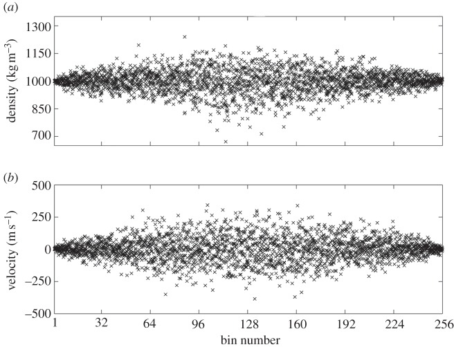
As an illustration of TARDIS's application to resolving nanoscale thermal velocity fluctuations in the region of interest of microscale-size channel flow on a grid of 200×200 control volumes, figure 1 shows the velocity profile through two cross sections along the height of the channel. These plots show that the fluctuations are most evident in the centre of the domain, corresponding to the small scales (CS2). In the large-scale part of the domain (CS1), the fluctuations become almost indistinguishable from the background Poiseuille flow profile. Figure 2 shows the results of TARDIS application for modelling of thermal density fluctuations in water at equilibrium conditions when the spatial length scale of the control volume ranges from eight atoms in the centre of the domain to 2190 atoms near the boundaries. For this calculation, the TARDIS grid is 256×10 control volumes. The problem considered corresponds to the grand canonical ensemble of volume V _c (size of the control volume) and temperature T, for which the following linear relationship between the standard deviation of density fluctuations and the inverse of isothermal sound speed c_T (1510 m s⁻¹ for water at normal conditions) is valid [23]:

2.9

For the entire range of scales considered, the standard deviation of density that is computed from the LL-FH solution satisfies the theoretical relation within a few per cent error, which is within the statistical noise level (figure 3).

Figure 1.

Simulation results with fluctuating hydrodynamics, comparison with the theory. CS2 corresponds to the small-scale part of the domain and CS1 corresponds to large scales. (Online version in colour.)

Figure 2.

Simulation results for thermal fluctuations in water at equilibrium conditions for a range of control volumes (bins number 1 and 256 correspond to the largest control volumes and bin number 128 corresponds to the smallest ones): instantaneous (a) density and (b) x-velocity component fluctuations.

Figure 3.

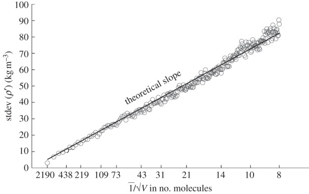
Simulation results for thermal fluctuations in water at equilibrium conditions for a range of control volumes: standard deviation of density fluctuations as a function of the system size.

(b). The role of density fluctuations in the dynamics of biomolecules: molecular dynamics results

We have simulated a system consisting of a dialanine zwitterion in a bath of explicit water. Classical MD has been used with the SPC (simple point charge) water model and the united-atom force field GROMOS for the peptide. The GROMACS software package was used for integrating the molecular equations of motion. The shape of the peptide is defined by the two dihedral angles (figure 4a). By calculating the ensemble-averaged density of water around the peptide (figure 4b), we aimed at answering the question: to what extent is the dynamics of water density connected with the dynamics of the peptide (quantified by its dihedral angles ϕ and ψ)?

Figure 4.

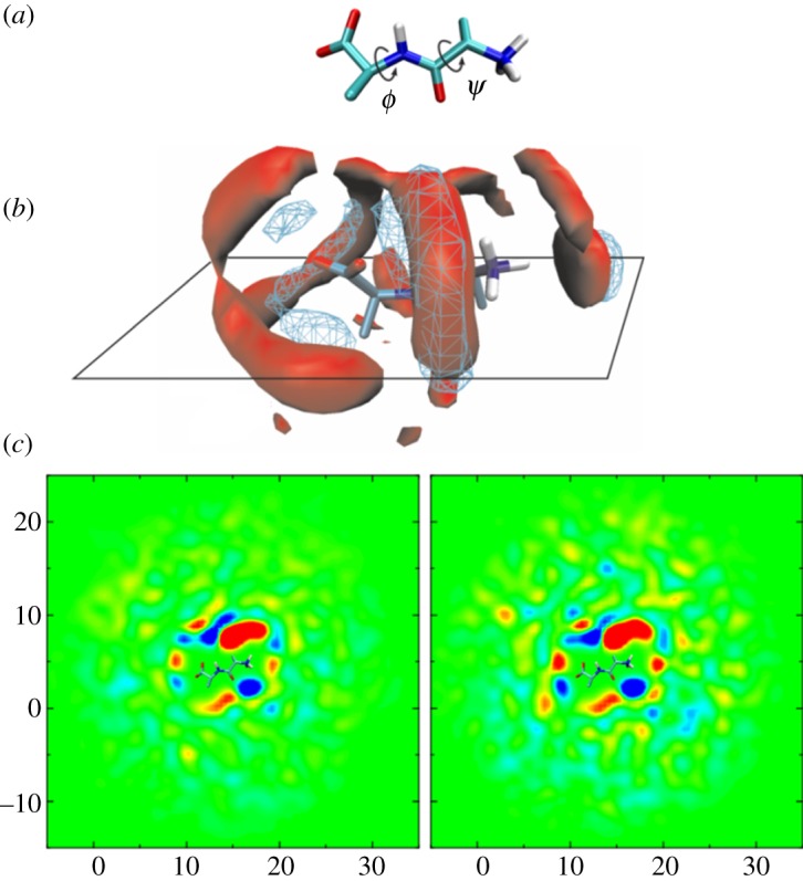
Water density fluctuations around a dialanine peptide. (a) The peptide molecule and two dihedral angles ϕ and ψ that define the shape of the molecule; (b) the same molecule together with oxygen (red) and hydrogen (blue mesh) densities around it; and (c) the projection of water density on the X–Y plane outlined in (b): right, the total density, left, the density dynamically correlated with the dihedral angles ϕ and ψ.

To answer the question, we first calculated the fluctuations of the water density field ρ(x,t) around its average value . We then analysed the dynamical correlations between the dihedral angles ϕ, ψ and the water density using the linear stochastic estimation (LSE) model, which was originally developed for visualizing coherent structures in turbulent flows [31] and the identification of noise sources in turbulent jets [32]. In this approach, an approximation to ρ′ is found that minimizes the error [33], where are the angles averaged over all the frames at time t, α,β are stationary fields, and quantifies the density fluctuations correlated with the angles. The system of linear equations is solved to calculate the constants α,β:

2.10

and

2.11

Figure 4c shows the original density fluctuations field ρ′(x,t) on the right together with its part correlated with the peptide conformations on the left. The correlations are very strong in the first hydration shell of the biomolecule and remain non-negligible at a significant distance from it. Moreover, as we have shown [14], these correlations are qualitatively different in various regimes of the peptide's dynamics: they are strong at the moments of conformational transitions (when the shape of the peptide changes significantly) and weak at the times of metastable fluctuations of the peptide around the same average shape. Thus, the microscopic fluctuations not only are non-negligible, but also constitute the essence of the molecular phenomenon.

Summarizing, these above subsections clearly demonstrate that it is possible to accurately calculate the fluctuations of the liquid at the scales where the hydrodynamic and atomistic descriptions overlap and these fluctuations are important for atomistic motions. This leads to the question of how both continuum and atomistic descriptions can be implemented within the same multiscale framework, as discussed in §4.

3. Coupling of the Landau–Lifshitz fluctuating hydrodynamics and molecular dynamics equations based on a hydrodynamic analogy

(a). Theory

Consistent coupling of the LL-FH model with MD equations remains a problem since the existing LL-FH–MD approaches [22] share the drawbacks of many other hybrid approaches, where a combination of artificial repulsive wall boundary condition based on a constrained particle dynamics concept and/or a particle reservoir with periodic boundaries is used. The latter prevents particles from drifting away, but may introduce spurious correlations and limits the geometry of the MD region. One of the questions that emerges for coupling LL-FH and MD is the choice of a hybrid modelling strategy that allows a smooth reduction of the number of degrees of freedom from fine scales (MD model) to large scales (LL-FH model). Essentially, this is the problem of developing a suitable low-order model for reducing the complexity of the MD model to the LL-FH framework based on Gaussian statistics in the macroscopic limit. On the other hand, mathematical modelling approaches based on low-order models have been used in continuum fluid dynamics for several decades. A classic example is the Lighthill acoustic analogy, which was introduced to bridge the scale difference that spans three to four orders of magnitude between the sound waves in the range of audible frequencies and the turbulent flow structures that generate sound. Since the pioneering work of Lighthill [34] various hybrid methods of this kind have been introduced in the literature. They all share a general idea to exactly rearrange the governing NS equations into the form of non-homogeneous linear equations and a nonlinear source at the right-hand side. For most advanced approaches of this type [35–37], the nonlinear source is directly related to the properties of fine-scale solution (space–time scales of the turbulence). In this work, the model based on a hydrodynamic analogy with two-phase flows is proposed for coupling the LL-FH and MD equations.

Let us consider a nominally two-phase liquid. The two phases are a Lagrangian and an Eulerian representation of the same chemical substance, which correspond to the atomistic (MD) and the continuum (LL-FH) model, respectively (figure 5). The phases are immersed into each other as ‘fine grains’, the surface tension effects are irrelevant, and both phases simultaneously occupy the same control volume. The partial concentrations of the MD ‘phase’ and the LL-FH ‘phase’ are equal to s and 1−s, respectively, where s is a parameter of the model, 0≤s≤1. In general, s is a user-defined scale function of space and time, which controls how much atomistic information is required in a particular region of the simulation domain.

Figure 5.

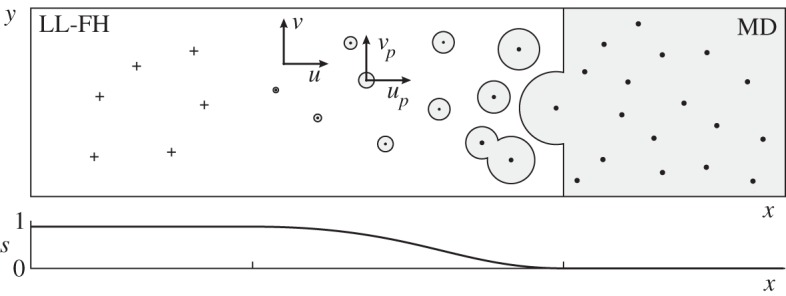
Schematic of the hybrid LL-FH/MD model: by entering the hybrid LL-FH/MD zone the MD particles lose some part of their pair potential interaction and become partially driven by the continuum LL-FH force field.

For simplicity, let us consider the case of liquids for which the adiabatic heat ratio approaches unity, and the first two equations for mass and momentum in the LL-FH equation (2.1) can be solved separately from the energy equation [23]. Following the standard approach in two-phase modelling [38], the conservation laws for the mass of each phase are given by

3.1

and

3.2

Here ρ_p=m_p/V is the effective density of MD particle p that occupies elementary control volume V , corresponding to the grand canonical ensemble for the LL-FH model, ρ is LL-FH phase density, m_p is particle mass, u_p is the MD velocity, is the average velocity of the mixture , where u_i is the velocity of the continuum LL-FH phase, N is the number of particles per control volume V and J^(ρ) is the mass source/sink term which describes the phase transition. The latter describes the exchange of mass between the MD and LL-FH models, which needs to be defined. It is easy to see that (3.1) and (3.2) automatically satisfy the conservation law of the total mass of the liquid, .

In a similar manner, the momentum equations of the two phases are introduced as

3.3

and

3.4

where F_ip is the MD force exerted on particle p due to the pair potential interactions, for which an explicit expression is not required in the model as will be discussed later, and J^(u) is the LL-FH/MD momentum exchange term. Similar to J^(ρ), J^(u) is a hybrid model quantity to be defined. By combining (3.3) and (3.4), it can be seen that Newton's second law, which equates the change of the total momentum , where to the force applied, is satisfied if for each control volume.

To close the model, the source/sink terms in the mass and momentum equations J^(ρ) and J^(u) must be defined. These terms are specified so that the conserved mass and momentum per each control volume V , and are driven towards the macroscopic averages obtained from the MD simulation in the hybrid MD/LL-FH zone, 0<s<1:

3.5

Here , and L^(ρ)(⋅) and L^(u)(⋅) are some operators, which play the role of LL-FH/MD boundary conditions to drive the corresponding deviations to the prescribed values within the hybrid MD/LL-FH zone 0<s<1 and return zero value for s=0 and s=1. For s=1 and no MD particles, it is easy to see that the solution of (3.3) converges to the continuum LL-FH model.

For equilibrium, when there are no external macroscopic forces, the continuum force term is equal to zero in accordance with the fluctuation–dissipation theorem. For non-equilibrium, this continuum force term is equal to the external force.

For the current implementation, several models for L^(ρ)(⋅) and L^(u)(⋅) have been tested, which correspond to driving the difference between the continuum average state and the MD average to zero using either (soft) diffusive or (hard) exponential forcing, (3.6) and (3.6a), respectively:

3.6

3.6a

where α,β>0 are numerical adjustable parameters.

The soft diffusive forcing (3.6) leads to the best results in terms of the hybrid algorithm's robustness and accuracy for a good of range of parameters 50<α,β<2000 (in reduced units specified in table 1) and 0<s<1.

Table 1.

Reduced units for argon liquid.

time	2.1502×10−12 s
density	1.6410×103 kg m−3
velocity	159.61 m s−1
temperature	122.4 K
force	4.9240×10−12 N
stress	41.805 MPa
number of atoms	10 000
number of LL-FH cells	5×5 with 400 atoms per cell size

From (3.5) and (3.6), the MD/LL-FH phase source terms J^(ρ) and J^(u) in the continuum FF-LH equations (3.1) and (3.3) are obtained as

3.7

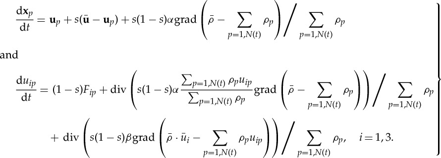
To complete the hybrid model description (3.1)–(3.4), one needs to modify the classical MD equations dx_p/dt=u_p,du_p/dt=F_p, where x_p, u_p and F_p are the coordinate, velocity and pair potential force applied to the particle, so that there is an exact correspondence between (3.7), which satisfies the governing equations for the LL-FH phase (3.1), equation (3.3) and the sink sources in the macroscopic conservation laws for MD particles, (3.2) and (3.4).

This is achieved by the following modification of the MD equations:

3.8

The above relations for the modified MD particle velocity and acceleration, dx_p/dt and du_ip/dt, have been derived starting from the conservation of mass and the corresponding equation for velocity and acceleration of the MD particles per control volume

3.9

and then exactly rearranging these equations to the form of macroscopic conservation laws (3.2) and (3.4) where the sink terms are given by (3.8).

Notably, in comparison with constrained particle dynamics models used in the literature [17], the current model (i) preserves a strict conservation of mass and momentum and (ii) in the continuum limit s→1, it correctly captures the mean and the variance of thermal fluctuations due to its convergence to the LL-FH equations.

For numerical implementation, the system of equations (3.1), (3.2) and (3.4) is solved with an explicit time-marching scheme where the MD and LL-FH solution parts are updated concurrently.

(b). Numerical implementation results

For the current proof of concept study, liquid argon has been simulated for equilibrium conditions at temperature T=2.4 and mean density ρ=0.607. The reduced units are used and the main numerical parameters are summarized in table 1.

To initialize the solution, 50 000 MD iterations are first performed with a Nosé–Hoover thermostat [39,40] to reach the prescribed macroscopic parameters, after which the thermostat is turned off and the hybrid model simulations are conducted. There are about 2 000 000 MD time steps performed in total and 1 000 000 MD time steps are typically required to reach statistical convergence within 5%. The exchange between the continuum phase (FH) and the MD phase solutions is performed at every 10th MD step (MD step is equal to 1/10th of FH step) and statistics are collected every 50 time steps as in [24] for faster convergence. To investigate the hybrid model accuracy for multi-time stepping, the same model has also been tested by reducing the FH step so that one MD steps correspond to one FH step. The accuracy of the hybrid model in predicting the statistics of fluctuations remains fairly insensitive to the change of the FH step.

The simulations of the current hybrid LL-FH/MD model have been performed for several values of the model parameters, 50<α,β<2000 and 0<s<1. In all cases, a two-dimensional periodic box solution domain is considered. Figure 6 shows a typical behaviour of the standard deviation (std) of conservative velocity variable for i=1 that corresponds to the x-velocity component as a function of the number of MD iterations. Two representative values of the hybrid model parameter are considered. One corresponds to the case when the hybrid model is mostly driven by macroscopic dynamics (s=0.8). The other corresponds to the case when the hybrid model is mostly driven by MD dynamics (s=0.1). For reference, the pure atomistic MD solution and the pure continuum LL-FH solution of the same problem are shown on the same graph.

Figure 6.

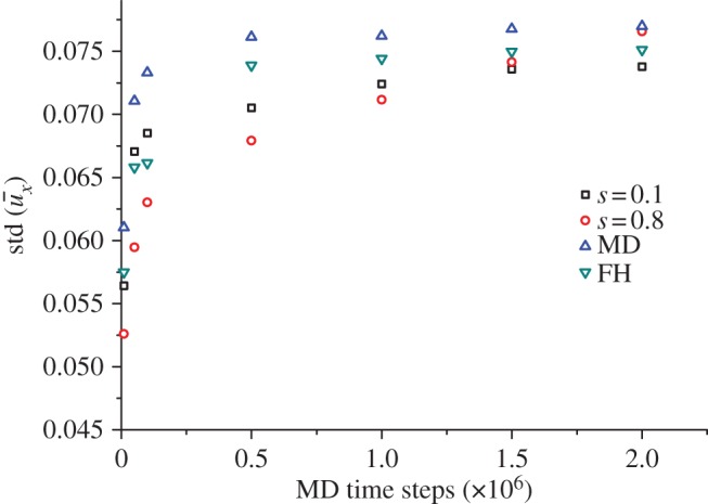
The convergence of the standard deviation of the velocity x-component with the number of MD time steps for the current hybrid model at s=0.1 and s=0.8 (conservative velocity variable) and the reference pure MD and FH models. (Online version in colour.)

It can be seen that the hybrid model solution converges to the reference value of the pure MD solution and that of the pure LL-FH solution within the statistical uncertainty for both cases. For the solutions shown, α,β=50, but it has also been checked that a similar convergence to the correct limit can be obtained for α,β=2000.

To investigate the hybrid model's capability to deal with the situation when the hybrid system is not in equilibrium initially, the following test case has been considered.

The previous system of liquid argon is simulated when the continuum part of the solution is initially given a certain mean flow velocity drift while the MD part of the solution is initialized with no drift. Figure 7 shows the behaviour of the two parts of the solution for s=0.5. Having started from two different initial average velocities, the two parts of the hybrid model converge in the middle. This behaviour is completely consistent with the preservation of the mean flow rate that is expected in the model.

Figure 7.

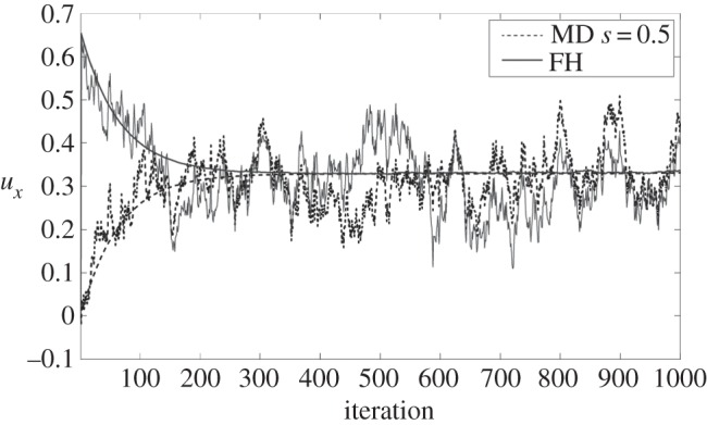
Velocity convergence for the case of starting the hybrid model with an initial drift specified in the x-component of the continuum (FH) part of the solution while the MD solution is initialized with no drift. The solutions for a single control volume and the solution averaged over all control volumes are shown. Each iteration corresponds to 50 MD time steps.

4. Conclusion

A new self-consistent hybrid MD-CH modelling framework based on an analogy with two-phase hydrodynamics is developed. For this framework, the MD equations are constrained so that their macroscopic behaviour satisfies the boundary conditions in the hybrid LL-FH/MD zone with a strict conservation of macroscopic mass and momentum throughout the solution domain.

The course-graining parameter, s, is introduced into the governing equations by an analogy with the two-phase hydrodynamics to permit a very natural treatment of the scale differences in the MD and the LL-FH representations. The LL-FH model for macroscopic flow description allows the statistics of thermal velocity fluctuations to be captured for a wide range of control volumes from 8 to 2190 atoms per cell length. Its implementation can be as efficient as that of the conventional deterministic CFD methods by using non-uniform Eulerian grids and asynchronous time stepping. Microscopic fluctuations that can be captured by the LL-FH model not only are non-negligible, but also constitute the essence of the molecular phenomenon, as demonstrated for modelling of a dialanine zwitterion in a bath of explicit water.

The new hybrid LL-FH/MD method is implemented for the simulation of liquid argon at equilibrium conditions. The method is shown to produce a converged solution that correctly captures macroscopic parameters such as standard deviation of thermal fluctuations and the mean flow velocity. This is achieved without introducing any ad-hoc treatment of MD particles such as ‘rescaling’ of the MD solution.

At present, the MD part of the current hybrid LL-FH/MD method is limited to a box domain where the average number of MD particles is maintained the same in all control volumes including the part of the computational domain that is dominated by continuum dynamics. Future work will be devoted to extending the current implementation to multi-time-scale modelling of the MD particles. One possibility for multiscale treatment of MD particles can include their gradual coarse-graining in the continuum part of the domain (s→1) so that the individual atoms there gradually become ‘hard spheres’, their response time to the pair potential force increases accordingly, and their dynamics is governed by the continuum LL-FH field.

Once fully implemented, it is expected that the new hybrid LL-FH/MD approach will become an efficient tool for multiscale simulations of biomolecules in liquids such as the simulation of hydrodynamic control of protein conformations in microfluidic devices.

Funding statement

This work has been supported in the framework of the G8 Research Councils Initiative on Multilateral Research Funding (Engineering and Physical Sciences Research Council grant no. EP/J004308/1) and Russian Foundation for Basic Research (11–07–93938-G8_a).

References

- 1.Batchelor GK. 1967. An introduction to fluid dynamics. Cambridge, UK: Cambridge University Press. [Google Scholar]
- 2.Golse F. 2006. The Boltzmann equation and its hydrodynamic limits. Handb. Diff. Equ. Evol. Equ. 2, 159–301. ( 10.1016/S1874-5717(06)80006-X) [DOI] [Google Scholar]
- 3.Brody JP, Yager P, Goldstein RE, Austin RH. 1996. Biotechnology at low Reynolds numbers. Biophys. J. 71, 3430–3441. ( 10.1016/S0006-3495(96)79538-3) [DOI] [PMC free article] [PubMed] [Google Scholar]
- 4.Shapiro E, Drikakis D, Gargiuli J, Vadgama P. 2007. Interface capturing in dual-flow microfluidics. J. Comput. Theor. Nanosci. 4, 1–5. ( 10.1166/jctn.2007.001a) [DOI] [Google Scholar]
- 5.Ivorra B, Redondo JL, Santiago JG, Ortigosa PM, Ramos AM. 2013. Two- and three-dimensional modeling and optimization applied to the design of a fast hydrodynamic focusing microfluidic mixer for protein folding. Phys. Fluids 25, 032001 ( 10.1063/1.4793612) [DOI] [Google Scholar]
- 6.Gaudet M, Remtulla N, Jackson SE, Main ERG, Bracewell DG, Aeppli G, Dalby PA. 2010. Protein denaturation and protein: drugs interactions from intrinsic protein fluorescence measurements at the nanolitre scale. Protein Sci. 19, 1544–1554. ( 10.1002/pro.433) [DOI] [PMC free article] [PubMed] [Google Scholar]
- 7.Koplik J, Banavar JR. 1995. Continuum deductions from molecular hydrodynamics. Annu. Rev. Fluid Mech. 27, 257–292. ( 10.1146/annurev.fl.27.010195.001353) [DOI] [Google Scholar]
- 8.Mansur E, Ye M, Wang Y, Dai Y. 2008. A state-of-the-art review of mixing in microfluidic mixers. Chin. J. Chem. Eng. 16, 503–516. ( 10.1016/S1004-9541(08)60114-7) [DOI] [Google Scholar]
- 9.Fritsch S, Poblete S, Junghans C, Ciccotti G, Delle Site L, Kremer K. 2012. Adaptive resolution molecular dynamics simulation through coupling to an internal particle reservoir. Phys. Rev. Lett. 108, 170602 ( 10.1103/PhysRevLett.108.170602) [DOI] [PubMed] [Google Scholar]
- 10.di Pasquale N, Marchisio D, Carbone P. 2012. Mixing atoms and coarse-grained beads in modelling polymer melts. J. Chem. Phys. 137, 164111–164119. ( 10.1063/1.4759504) [DOI] [PubMed] [Google Scholar]
- 11.Kumar P, Franzese G, Buldyrev SV, Stanley EH. 2006. Molecular dynamics study of orientational cooperativity in water. Phys. Rev. E 73, 041505 ( 10.1103/PhysRevE.73.041505) [DOI] [PubMed] [Google Scholar]
- 12.Umezawa K, Morikawa R, Nakamura H, Higo J. 2010. Solvent flow patterns fluctuating largely around a protein and correlation with solvent density fluctuations: a molecular dynamics study. J. Chem. Phys. 132, 155103 ( 10.1063/1.3378263) [DOI] [PubMed] [Google Scholar]
- 13.Frauenfelder H, Chen G, Berendzen J, Fenimore PW, Jansson H, McMahon BH, Stroe IR, Swenson J, Young RD. 2009. A unified model of protein dynamics. Proc. Natl Acad. Sci. USA 106, 5129–5134. ( 10.1073/pnas.0900336106) [DOI] [PMC free article] [PubMed] [Google Scholar]
- 14.Nerukh D, Karabasov S. 2013. Water–peptide dynamics during conformational transitions. J. Phys. Chem. Lett. 4, 815–819. ( 10.1021/jz400051p) [DOI] [PubMed] [Google Scholar]
- 15.O'Connell S, Thompson P. 1995. Molecular dynamics–continuum hybrid computations: a tool for studying complex fluid flows. Phys. Rev. E 52, 5792–5795. ( 10.1103/PhysRevE.52.R5792) [DOI] [PubMed] [Google Scholar]
- 16.Flekkoy EG, Wagner G, Feder J. 2000. Hybrid model for combined particle and continuum dynamics. Europhys. Lett. 52, 271–276. ( 10.1209/epl/i2000-00434-8) [DOI] [Google Scholar]
- 17.Nie XB, Chen SY, Robbins MO. 2004. A continuum and molecular dynamics hybrid method for micro- and nano-fluid flow. J. Fluid Mech. 500, 55–64. ( 10.1017/S0022112003007225) [DOI] [Google Scholar]
- 18.Hadjiconstantinou NG. 1999. Hybrid atomistic–continuum formulations and the moving contact-line problem. J. Comput. Phys. 154, 245–265. ( 10.1006/jcph.1999.6302) [DOI] [Google Scholar]
- 19.Asproulis A, Kalweit M, Drikakis D. 2012. A hybrid molecular continuum method using point wise coupling. Adv. Eng. Softw. 46, 85–92. ( 10.1016/j.advengsoft.2010.10.010) [DOI] [Google Scholar]
- 20.Steijl R, Barakos G. 2012. Coupled Navier–Stokes/molecular dynamics simulations in nonperiodic domains based on particle forcing. Int. J. Numer. Meth. Fluids 69, 1326–1349. ( 10.1002/fld.2641) [DOI] [Google Scholar]
- 21.Landau LD, Lifshitz EM. 1980. Statistical physics part 1 Amsterdam, The Netherlands: Elsevier. [Google Scholar]
- 22.De Fabritiis G, Delgado-Buscalioni R, Coveney PV. 2006. Multiscale modeling of liquids with molecular specificity. Phys. Rev. Lett. 97, 134501 ( 10.1103/PhysRevLett.97.134501) [DOI] [PubMed] [Google Scholar]
- 23.De Fabritiis G, Serrano M, Delgado-Buscalioni R, Coveney PV. 2007. Fluctuating hydrodynamic modeling of fluids at the nanoscale. Phys. Rev. E 75, 026307 ( 10.1103/PhysRevE.75.026307) [DOI] [PubMed] [Google Scholar]
- 24.Voulgarakis NK, Chu J-W. 2009. Bridging fluctuating hydrodynamics and molecular dynamics simulations of fluids. J. Chem. Phys. 130, 134111 ( 10.1063/1.3106717) [DOI] [PubMed] [Google Scholar]
- 25.Ladd JC. 1993. Short-time motion of colloidal particles: numerical simulation via a fluctuating lattice-Boltzmann equation. Phys. Rev. Lett. 70, 1339–1342. ( 10.1103/PhysRevLett.70.1339) [DOI] [PubMed] [Google Scholar]
- 26.Español P. 1997. Dissipative particle dynamics with energy conservation. Europhys. Lett. 40, 631 ( 10.1209/epl/i1997-00515-8) [DOI] [Google Scholar]
- 27.Landau LD, Lifshitz EM. 1987. Fluid mechanics, vol. 6, 2nd edn. London, UK: Butterworth–Heinemann. [Google Scholar]
- 28.Markesteijn AP, Karabasov SA. 2014. Time asynchronous relative dimension in space method for multi-scale problems in fluid dynamics. J. Comput. Phys. 258, 137–164. ( 10.1016/j.jcp.2013.10.035) [DOI] [Google Scholar]
- 29.Omelchenko YA, Karimabadi H. 2006. Self-adaptive time integration of flux-conservative equations with sources. J. Comput. Phys. 216, 179–194. ( 10.1016/j.jcp.2005.12.008) [DOI] [Google Scholar]
- 30.Dawson C, Kirby R. 2001. High resolution schemes for conservation laws with locally varying time steps. SIAM J. Sci. Comput. 22, 2256–2281. ( 10.1137/S1064827500367737) [DOI] [Google Scholar]
- 31.Adrian RJ. 1994. Stochastic estimation of conditional structure: a review. Appl. Sci. Res. 53, 291–303. ( 10.1007/BF00849106) [DOI] [Google Scholar]
- 32.Kerherve F, Jordan P, Cavalieri AVG, Delville J, Bogey C, Juve D. 2012. Educing the source mechanism associated with downstream radiation in subsonic jets. J. Fluid Mech. 710, 606–640. ( 10.1017/jfm.2012.378) [DOI] [Google Scholar]
- 33.Papoulis A, Pillai S. 2002. Probability, random variables and stochastic processes. New York, NY: McGraw-Hill. [Google Scholar]
- 34.Lighthill MJ. 1952. On sound generated aerodynamically. I. General theory. Proc. R. Soc. Lond. A 222, 564–587. ( 10.1098/rspa.1952.0060) [DOI] [Google Scholar]
- 35.Goldstein ME. 2003. A generalized acoustic analogy. J. Fluid Mech. 488, 315–333. ( 10.1017/S0022112003004890) [DOI] [Google Scholar]
- 36.Goldstein ME, Leib SJ. 2008. The aero-acoustics of slowly diverging supersonic jets. J. Fluid Mech. 600, 291–337. ( 10.1017/S0022112008000311) [DOI] [Google Scholar]
- 37.Karabasov SA. 2010. Understanding jet noise. Phil. Trans. R. Soc. A 368, 3593–3608. ( 10.1098/rsta.2010.0086) [DOI] [PubMed] [Google Scholar]
- 38.Buckley SE, Leverett MC. 1942. Mechanism of fluid displacements in sands. Trans. AIME 146, 107–116. [Google Scholar]
- 39.Nosé J. 1984. A unified formulation of the constant temperature molecular dynamics methods. Chem. Phys. 81, 511 ( 10.1063/1.447334) [DOI] [Google Scholar]
- 40.Hoover W. 1985. Canonical dynamics: equilibrium phase-space distributions. Phys. Rev. A 31, 1695 ( 10.1103/PhysRevA.31.1695) [DOI] [PubMed] [Google Scholar]