Statistics and Related Topics in Single-Molecule Biophysics

Abstract

Since the universal acceptance of atoms and molecules as the fundamental constituents of matter in the early twentieth century, molecular physics, chemistry and molecular biology have all experienced major theoretical breakthroughs. To be able to actually “see” biological macromolecules, one at a time in action, one has to wait until the 1970s. Since then the field of single-molecule biophysics has witnessed extensive growth both in experiments and theory. A distinct feature of single-molecule biophysics is that the motions and interactions of molecules and the transformation of molecular species are necessarily described in the language of stochastic processes, whether one investigates equilibrium or nonequilibrium living behavior. For laboratory measurements following a biological process, if it is sampled over time on individual participating molecules, then the analysis of experimental data naturally calls for the inference of stochastic processes. The theoretical and experimental developments of single-molecule biophysics thus present interesting questions and unique opportunity for applied statisticians and probabilists. In this article, we review some important statistical developments in connection to single-molecule biophysics, emphasizing the application of stochastic-process theory and the statistical questions arising from modeling and analyzing experimental data.

1 Introduction

Although the concept of atoms and molecules can be traced back to ancient Greece, the corpuscular nature of atoms was firmly established only in the beginning of the 20th century. The stochastic movement of molecules and colloidal particles in aqueous solutions, known as the Brownian motion, explained by the diffusion theory of A. Einstein (1905) and M. von Smoluchowski (1906), and the stochastic differential equation of P. Langevin (1908) – confirmed experimentally through the statistical measurements of J.-B. Perrin (1912), T. Svedberg and A.F. Westgren (1915) – played a decisive role in its acceptance [1]. The literature on this subject is enormous. We refer the readers to the excellent edited volume [2], which included now classical papers by Chandrasekhar, Uhlenbeck-Ornstein, Wang-Uhlenbeck, Rice, Kac and Doob, and [3], a collection of lectures by Kac, one of the founding members of the modern probability theory [4].

While physicists, ever since Isaac Newton, have been interested in the position and velocity of particle movements, chemists have always perceived molecular reactions as discrete events, even though no one had seen it until the 1970s. Two landmark papers that marked the beginning of statistical theories in chemistry (at least in the U.S.) appeared in the 1940s [5, 6]. Kramers' paper [5] elucidated the emergence of a discrete chemical transition in terms of a continuous “Brownian motion in a molecular force field” with two stable equilibria separated by an energy saddle and derived an asymptotic formula for the reaction rate. Probabilistically speaking, this is the rate of an elementary chemical reaction as a rare event [7]. Delbrück's paper [6] assumed discrete transitions with exponential waiting time for each and every chemical reaction and outlined a stochastic multi-dimensional birth-and-death process for a chemical reaction system with multiple reacting chemical species. Together, these two mathematical theories have established a path from physics to cell biology by (i) bridging the atomic physics with individual chemical reactions in aqueous solutions, and (ii) connecting coupled chemical reactions with dynamic chemical/biochemical systems. In 1977, Gillespie independently discovered Delbrück's chemical master equation approach [8] in terms of its Markovian trajectories based on a computational sampling algorithm now bears his name in the biochemistry community [9]. The simulation method actually can be traced back to Doob [10].

Experimental techniques have experienced major breakthroughs along with these theoretical developments. J.-B. Perrin's investigations on Brownian motion gave perhaps the first set of single-particle measurements with stochastic trajectory. The spatial and temporal resolutions back in 1910s were on the order of micrometer and tens of second. By the late 1980s, they became nanometer and tens of millisecond. The observation of discrete stochastic transitions between different states of a single molecule was first achieved in the 1970s on ion channels, proteins imbedded in the biological cell membrane. This was made possible by the invention of the patch-clamp technique, together with the exquisite electronics, for measuring small electrical current [11]. To measure the stochastic dynamics of a “tumbling” single molecule in an aqueous solution, one needs to be able to “see” the molecule under a microscope for a sufficiently long time. For this purpose, one needs an experimental technique to immobilize a molecule and a highly sensitive optical microscopy. This was first accomplished for enzyme molecules at room temperature in 1998 [12].

To statisticians and probabilists, this is abundantly clear that biophysical dynamics at the molecular level are stochastic processes. To characterize such dynamics, called fluctuations in chemical physics literature, one thus needs stochastic models. In an experiment, if such processes are sampled over time, one molecule at a time, then the analysis of experimental data naturally calls for the inference of stochastic processes. Therefore, the theoretical and experimental developments of single-molecule biophysics constitute one great opportunity for applied statistics and probabilities.

The aim of this article is to review some important statistical developments in single-molecule biophysics from the construction of theoretical models to advances in the experiments, mostly drawing from our own limited research experience. The discussion is far from complete, as the field of single-molecule biophysics, with a substantial background, is advancing too rapidly to be captured by a short review. Still, we hope to convey a certain amount of historical continuity, as well as current excitement at the research interface between statistics and molecular biophysics. Special attention is paid to the application of stochastic-process theory and the statistical questions arising from analyzing experimental data.

In the presentation we discuss the underlying theory, the experiments as well as the analysis of experimental data. The discussion of theory focuses more on the application of stochastic processes in modeling various problems in single-molecule biophysics, whereas the discussion of experiments and data focuses more on the statistical analysis of data. However, we want to emphasize that, as one observes in the advance of modern sciences, theory and experiment/data really go hand in hand: the development in one stimulates and inspires the other.

2 Brownian motion and diffusion of biological macromolecules

Before we discuss Brownian motion and its profound implications in biophysics, we want to first clarify the terminology, because the term “Brownian motion” used by physicists and chemists and the term “Brownian motion” used in probability and statistics refer to different things: physicists and chemists' Brownian motion corresponds to the integral of the Ornstein-Uhlenbeck process (as we shall see shortly), whereas statisticians and probabilists' Brownian motion refers to the Wiener process, although both share the characteristic of E[x²(t)]∝ t for large t. Likewise, “diffusion” has different meaning in statistics and biophysics. In statistics and probability, the term “diffusion processes” typically refers to continuous-time and continuous-space Markov processes, such as Itō's diffusions. In biophysics, the term “diffusion” typically refers to physical motion of a particle without an external potential; when there is a drift, it is often called biased diffusion.

To facilitate our discussion, let us first review the derivation of the law of physical Brownian motion [7]. Suppose we have a particle with mass m suspended in a fluid. Then according to Newton's equation of motion formulated by Langevin, the velocity v(t) of the particle satisfies

$$m\frac{\mathit{\text{dv}}(t)}{\mathit{\text{dt}}}=-\zeta v(t)+F(t),$$ (1)

where ζ is the damping coefficient and F(t) is a white noise – formally the “derivative” of the Wiener process. To correctly represent an inert particle in thermal equilibrium with the fluid, the Langevin equation has an important physical constraint that links the damping coefficient ζ with the noise level, because both the movement of the particle and the friction originate from one source – the collision between the particle and surrounding fluid molecules:

$$E[F(t)F(s)]=2\zeta k_{B}T\cdot \delta (t-s),$$ (2)

where δ(·) is Dirac's delta function, k_B is the Boltzmann constant, and T is the underlying temperature. Equation (2) is a consequence of the fluctuation-dissipation theorem in statistical mechanics [13]. Probabilistically speaking, a Markov-process model for an inert system that tends to thermal equilibrium is necessarily reversible [14, 15].

In the more rigorous probability notation, equations (1) and (2) translate to

$$m\mathit{\text{dv}}(t)=-\zeta v(t)\mathit{\text{dt}}+\sqrt{2\zeta k_{B}T}\mathit{\text{dB}}(t),$$ (3)

where B(t) is the Wiener process, and the formal association of “ $F(t)=\sqrt{2\zeta k_{B}T}\mathit{\text{dB}}(t)/\mathit{\text{dt}}$” is recognized. The stationary solution of equation (3) is the Ornstein-Uhlenbeck process [2], which is Gaussian with mean function E[v(t)] = 0 and covariance function $E[v(t)v(s)]=\frac{k_{B}T}{m}exp\left(-\frac{\zeta }{m}\left|t-s\right|\right)$. It follows that for the displacement, $x(t)={\int }_0^{t}v(s)\mathit{\text{ds}}$, which can be recorded in single-particle tracking, its mean squared is

$$\begin{array}{lll}E[x^2(t)]\hfill & =\hfill & \text{Var}[x(t)]={\int }_0^t{\int }_0^{t}E[v(s)v(u)]\mathit{\text{du}}\mathit{\text{ds}}\hfill \\ \hfill & =\hfill & 2\left(\frac{k_{B}T}{\zeta }\right)t-2\left(\frac{k_B\mathit{\text{Tm}}}{{\zeta }^2}\right)\left(1-e^{-\frac{\zeta }{m}t}\right).\hfill \end{array}$$

Therefore,

$$E[x^2(t)]\sim \left(\frac{k_{B}T}{m}\right)t^2,\text{for small}t,$$ (4a)

$$E[x^2(t)]\sim 2\left(\frac{k_{B}T}{\zeta }\right)t,\text{for large}t.$$ (4b)

Equation (4b) gives the famous Einstein-Smoluchowski relation, which links the diffusion constant D with the “mobility” ζ of the particle D = k_BT/ζ. This equation is historically highly significant in that by combining it with Stokes' law, ζ = 6πηr, and the definition of the Boltzmann constant (k_B = R/N), one obtains

$$D=\frac{\mathit{\text{RT}}}{6\pi \eta \mathit{\text{rN}}},$$ (5)

where η is the viscosity, r is the radius of the spherical particle, R is the gas constant, and N is the Avogadro constant.

An immediate experimental consequence of (5) is that by measuring the diffusion constant of a spherical particle, one can estimate the Avogadro constant! The experiments on Brownian motions in fact had a rather shinning history in both physics and chemist. In 1926, Jean-Baptiste Perrin and Theodor Svedberg won the Nobel Prizes in physics and chemistry respectively. Perrin had studied trajectories of Brownian motions, verifying Einstein's description of Brownian motion and providing one of the first modern estimates of the Avogadro constant, while Svedberg developed the method of analytical ultracentrifugation using which he studied the counts of Brownian particles in a well-defined volume and how this counting process evolves over time. This counting process is referred to as the Smoluchowski process (first by M. Kac in [3]). Both Perrin and Svedberg's observations were performed on large colloids; it has to wait for nearly a half century for such measurements to be performed on biological macromolecules. A version of the Svedberg experiment appeared in the 1970s under the name of Fluorescence Correlation Spectroscopy (FCS, see Sec. 4), and the measurement of single trajectory was developed in the 1980s, known as Single-Particle Tracking (SPT), using the principle of “spatial high-resolution by centroid localization”. This principle is responsible for driving much of the recent advance in single-molecule biophysics and super-resolution imaging.

For experimental data from a true Brownian motion, a natural statistical question is to obtain estimates of the diffusion constant. If the data consist of the trajectories of individual particles as in SPT, the diffusion constant can be estimated by either a least-square regression or an MLE. Sec. 2.1 will discuss it in some detail. If the data consist of particle counting over time, the statistical estimation becomes more involved. We will discuss it in Sec. 3, starting with the Smoluchowski process, which is non-Markovian [16, 17].

In addition to estimating the diffusion constant, often the experimental objective is to investigate the motion that deviates from a simple Brownian motion. This has yielded a great deal of development in statistical treatments of these data: What if there is a drift, if the space is not homogeneous, if the Brownian particles can reversibly attach to other stationary or moving objects, or if the particles are interacting (e.g., not independent)? With the emerging of super-resolution imaging, these questions are still constantly being asked in laboratories; a systematic statistical treatment of the problem is yet to be developed [18].

2.1 Single-particle tracking of biological molecules

Since the late 1980s, camera-based single-particle tracking (SPT) has become a popular tool for studying the microscopic behavior of individual molecules [19]. The trajectory of an individual particle is typically recorded through a microscope by a digital camera in such experiments; the speed of the camera can be as fast as a few milliseconds per frame. The superb spatial resolution owes to the idea of centroid localization.

One of the most common statistical questions is to determine the diffusion constant D of the underlying particle from the experimental trajectory. If we denote (x(t₁), …, x(t_n)) the true positions of the particle at times t₁, …, t_n, where Δt ≡ t_i – t_i−1 is the time interval between successive positions, then the experimental observations (y₁, y₂, …, y_n) are y_i = x(t_i) + ε_i, where ${\epsilon }_i\stackrel{i.i.d.}{\sim }N(0,{\sigma }^2)$ are the localization (measurement) error. If the particle's motion is really Brownian, then, as we have seen in equation (4b) the process x(t) can be well approximated by $\sqrt{2D}B\left(t\right)$, where B(t) is the standard Wiener process, provided t ≫ m/ζ. This leads to

$$y_i=\sqrt{2D}B(t_i)+{\epsilon }_i.$$ (6)

An intuitive estimate of D used by many experimentalists utilizes the mean square displacement (MSD) [20], such as

$${\widehat{\rho }}_k=\frac{1}{2(n-k)k\mathrm{\Delta }t}\sum _{i=1}^{n-k}{(y_{i+k}-y_i)}^2,k=1,2,\dots ,$$

which are averages of correlated (square) increments, or

$${{\widehat{\rho }}^{\prime }}_k=\frac{1}{2\lfloor n/k\rfloor k\mathrm{\Delta }t}\sum _{i=1}^{\lfloor n/k\rfloor }{(y_{\mathit{\text{ik}}}-y_{1+(i-1)k})}^2,k=1,2,\dots ,$$

which are averages of nonoverlapping (square) increments. One can also try to combine them, for example, by weighting or a regression (against k) [21].

Given the parametric specification (6), another natural estimate of D is the maximum likelihood estimate (MLE) [22]. It is interesting to note that (i) MLE and the optimal estimate based on MSD have comparable accuracy [23], and (ii) the estimation error in D decreases with n, the sample size (the number of camera frames), at the rather slow rate of O(n^−1/4), which contrasts with the familiar rate of O(n^−1/2) as in the central limit theorem [24, 25, 26].

The determination of the diffusion constant D serves many purposes, ranging from (Perrin's original) estimation of the Avogadro constant to the test of whether the underlying motion is Brownian to the elucidation of detailed molecular mechanism. For example, Blainey et al. [27] studied how DNA-binding proteins move along DNA segments. Does a DNA-binding protein simply slide along the DNA, in which a protein executes simple one-dimensional translational move parallel to the DNA without rotation, or does a DNA-binding protein move along the DNA through a helical path, in which it retains a specific orientation with respect to the DNA helix and rotates with the helix (in a spiral fashion) [28, 29]? If we measure a protein's position along the DNA over time, then the two motions are subject to different expressions of the diffusion constant: in the parallel motion, the diffusion constant is

$$D=\frac{k_{B}T}{6\pi \eta r},$$

as we have seen in equation (5), where η is the viscosity and r is the size of the protein; in the helical motion, the diffusion constant is

$$D=\frac{k_{B}T}{\pi \eta r}{\left[6+{\left(\frac{2\pi }{b}\right)}^2\left(8r^2+6r_{\mathit{\text{oc}}}^2\right)\right]}^{-1},$$ (7)

where r_oc is the distance between the protein's center of mass and the axis of the DNA, and b is the distance along the DNA traveled by the protein per helical turn. Equation (7) is derived from hydrodynamic considerations [30, 31]. The parallel motion and helical motion can thus be told apart from the experimentally estimated diffusion constant. By tracking DNA-binding proteins with various sizes from different functional groups and estimating their diffusion constants from single-molecule experimental data, Blainey et al. [27] found that the helical motion is the general mechanism.

2.2 Subdiffusion

As we have seen in (4b), a key characteristic of Brownian motion is that the mean squared displacement E[x²(t)] ∝ t for moderate and large t. In some physical and biological systems [32, 33] the motion is observed to follow E[x²(t)] ∝ t^α with 0 < α < 1. These motions are referred to as subdiffusion because of α < 1. One theoretical approach to model subdiffusion is to employ fractional calculus (such as the use of fractional derivatives). This approach is reviewed in [34]. We review an alternative approach here: generalized Langevin equation with fractional Gaussian noise as postulated in [91].

We start with a generalized Langevin equation (GLE) [13]

$$m\frac{\mathit{\text{dv}}(t)}{\mathit{\text{dt}}}=-\zeta {\int }_{-\infty }^{t}v(u)K(t-u)\mathit{\text{du}}+G(t),$$ (8)

where, in comparison with the Langevin equation (1), (i) a noise G(t) having memory replaces the white noise, and (ii) the memory kernel K convoluted with the velocity makes the process non-Markovian. Owing to the fluctuation-dissipation theorem, the memory kernel K(t) and the noise are linked by [35]

$$E[G(t)G(s)]=k_{B}T\zeta \cdot K(t-s).$$

Note that the GLE reduces to the Langevin equation when K is the delta function.

Within the GLE framework, we are looking for a kernel function that can give subdiffusion. As the white noise is the formal “derivative” of a Wiener process, which is the unique process that satisfies (a) being Gaussian, (b) having independent increment, (c) having stationary increment, and (d) being self-similar, to generalize the white noise, a good candidate is a process with the properties of (a) Gaussian, (b) stationary increment and (c) self-similar. The only class of processes that embodies all three properties is the fractional Brownian motion (fBm) B_H(t) [36, 37], which has mean E[B_H(t)] = 0, and covariance $E[B_H(t)B_H(s)]=\frac{1}{2}(|t{|}^{2H}+|s{|}^{2H}-|t-s{|}^{2H})$. H ∈ [0, 1] is called the Hurst parameter. B_H(t) reduces to the Wiener process when H = 1/2.

Taking G(t) in (8) to be the (formal) derivative of fBm, $F_H(t)=\sqrt{2\zeta k_{B}T}{\mathit{\text{dB}}}_H(t)/\mathit{\text{dt}}$, we reach the model $m\frac{\mathit{\text{dv}}(t)}{\mathit{\text{dt}}}=-\zeta {\int }_{-\infty }^{t}v(u)K_H(t-u)\mathit{\text{du}}+F_H(t)$, where the kernel K_H(t) is given by

$$K_H(t)=E[F_H(0)F_H(t)]/(k_{B}T\zeta )=2H(2H-1)|t{|}^{2H-2},\text{for}t\ne 0.$$ (9)

F_H(t) is known as the fractional Gaussian noise (fGn).

In the more rigorous probability notation, the model can be written as

$$m\mathit{\text{dv}}(t)=-\zeta \left({\int }_{-\infty }^{t}v(u)K_H(t-u)\mathit{\text{du}}\right)\mathit{\text{dt}}+\sqrt{2\zeta k_{B}T}{\mathit{\text{dB}}}_H(t).$$ (10)

This equation is non-Markovian. Nevertheless, it can be solved in closed form via a Fourier analysis [38]. The solution v(t) is a stationary Gaussian process, and the displacement $x(t)={\int }_0^{t}v(s)\mathit{\text{ds}}$ satisfies

$$E[x{(t)}^2]=\text{Var}[x(t)]\sim \frac{k_{B}T}{\zeta }\left(\frac{2sin(2H\pi )}{\pi H(2H-1)(2H-2)}\right)t^{2-2H}\propto t^{2-2H},$$

for large t. Therefore, the model with H > 1/2 leads to subdiffusion.

If there exists an external potential U(x), a term −U′(x(t)) will be added to the right hand side of (8), yielding

$$\begin{array}{rrr}\hfill \mathit{\text{dx}}(t)& =\hfill & v(t)\mathit{\text{dt}}\hfill \\ m\mathit{\text{dv}}(t)\hfill & =\hfill & -\zeta \left({\int }_{-\infty }^{t}v(u)K_H(t-u)\mathit{\text{du}}\right)\mathit{\text{dt}}-U^{\prime }(x(t))\mathit{\text{dt}}+\sqrt{2\zeta k_{B}T}{\mathit{\text{dB}}}_H(t).\hfill \end{array}$$ (11)

For a harmonic potential $U(x)=\frac{1}{2}m\psi x^2$, the model can be solved by the Fourier transform method [38].

The subdiffusive motion is observed in single-molecule experiments on protein conformational fluctuation [39, 40]. The experiments studied the conformation fluctuation through the fluorescence lifetime of the protein. The fluorescence lifetime is a sensitive indicator, as it depends on the 3D atomic arrangements of the protein in an exponential way. The stochastic fluctuation of the fluorescence lifetime, recorded in the experiments, reveals the stochastic fluctuation in the protein's conformation. Detailed analysis of the autocorrelation, three-step and four-step correlation of the experimental fluorescence lifetime data shows that (i) the conformation fluctuation of the two protein systems undergo subdiffusion; (ii) the memory kernel is well described by equation (9), (iii) the conformation fluctuation is reversible in time, and (iv) a harmonic potential captures the fluctuation quite well. These subdiffusive observations, therefore, directly support the notation of fluctuating enzymes, also known as dynamic disorder – as an enzyme molecule spontaneously changes its conformation, its catalytic rate does not hold constant. The different conformations of an enzyme molecule and their intertransitions thus could have direct implications in the enzyme's catalytic behavior [41]. We will discuss some of those implications in Sec. 5.5. From a pure statistics standpoint, inference and testing the subdiffusive models beyond the autocorrelation function and three-step, four-step correlations are an open question.

3 Particle counting

The idea of counting the number of particles in a fixed region and using the temporal correlation of the resulting counting process to extract the kinetic parameters of the underlying experimental system has a long history, dating back to Smoluchowski's investigation of Brownian motion in the early twentieth century. Suppose we have indistinguishable particles, each undergoing independent Brownian motion. Let n(t) be the number of particles at time t in a region Ω (such as an area illuminated under a microscope). This counting process {n(t), t ≥ 0} is referred to as the Smoluchowski process. Under the assumption that the initial positions of the particles are uniformly distributed in a volume S (which is typically much larger than Ω), it can be shown that E(n(t)) = |Ω | / |S| and that for t ≫ m/ζ,

$$\text{Cov}(n(t),n(t+\tau ))=\frac{\left|\mathrm{\Omega }\right|}{\left|S\right|}\left\{1-\frac{1}{{(4\pi D\tau )}^{3/2}}{\iint }_{{\mathrm{x}}_1,{\mathrm{x}}_2\in \mathrm{\Omega }}exp\left(-\frac{{\Vert {\mathrm{x}}_1-{\mathrm{x}}_2\Vert }^2}{4D\tau }\right)d{\mathrm{x}}_{1}d{\mathrm{x}}_2\right\},$$ (12)

where |Ω| and |S| are the volumes of Ω and S, respectively, and D is the diffusion constant [3, 42, 43, 17, 44]. Note that under t ≫ m/ζ, the Brownian diffusion is well approximated by the Wiener process, which is the basis for equation (12). Historically, this result allowed the Brownian diffusion theory to be tested by particle counting – this was done notably by Svedberg and Westgren in the 1910s. It also allowed Smoluchowski to successfully account for the apparent “paradox” of microscopic reversibility of the motion of molecules and the macroscopic irreversibility as in the Second Law of Thermodynamics [45]. Finally, it offers an experimental way to determine the diffusion constant.

Estimating D from the experimentally observations (n(t₁), …, n(t_M)), where Δt ≡ t_i − t_i−1, is a statistical question. An intuitive method is to match the theoretical covariance function with the empirical one [42]:

$$\frac{1}{M-1}\sum _{i=2}^M{(n(t_i)-n(t_{i-1}))}^2=C(\mathrm{\Delta }t,D),$$ (13)

where C(Δt, D) is the right hand side of (12), which is a function of Δt and D. The solution D̂ of the generalized difference equation (13) is the estimate of D. Alternatively, one can also match lag-k square difference

$$\widehat{\mathit{\text{Cov}}}(k):=\frac{1}{M-k}\sum _{i=k+1}^M{(n(t_i)-n(t_{i-k}))}^2=C(k\mathrm{\Delta }t,D)$$

or use the nonlinear least square

$$arg\underset{D}{min}\sum _k{\left(\widehat{\mathit{\text{Cov}}}(k)-C(k\mathrm{\Delta }t,D)\right)}^2$$

or its (weighted) variation to estimate D [43].

The approach of using MLE to estimate D encounters the difficulty that the Smolochowski process is non-Markovian and that it does not have analytically tractable joint probability function. Approximating the Smolochowski process by an emigration-immigration (birth-death) process, which is Markovian, has been proposed [16, 17], where the birth rate and death rates can be set by making sure that the emigration-immigration and Smolochowski processes share the same mean and covariance (for small Δt). Systematic comparison between the two different estimation methods – the one based on empirical autocovariance function versus the quasi-likelihood estimate based on the emigration-immigration approximation – is an open question.

The scheme of counting particles and utilizing the temporal correlation to extract kinetic parameters was further developed into fluorescence correlation spectroscopy (FCS) in the 1970s, as we shall discuss in the next section, where, instead of the exact counts, the fluorescence level of the underlying system, which depends on the molecules' concentration, is recorded. The autocorrelation of the stochastic fluorescence reading can be used to estimate the parameters such as the diffusion constant and the reaction rate.

4 Fluorescence correlation spectroscopy and concentration fluctuations

With the development of laser-based microscope, one can now measure the number of molecules in a very small region within an aqueous solution and “count” the number of molecules: The counting is based on the fluorescent light emitted from the molecules. Assuming molecules are continuously giving out fluorescence, then the measurement of stationary fluorescence fluctuation from a small region provides information on concentration fluctuation. Since fluorescent emission requires excitation of an incoming light, the small region is naturally defined by the laser intensity function I(r), where r = (x, y, z) is the three-dimensional (3D) location of the particle [46]; I(r) can often be nicely represented by a Gaussian function $I(\mathbf{r})=I_{0}exp\left(-2(x^2+y^2)/{\omega }^2-2z^2/{\omega }_z^2\right)$.

For a collection of free-moving, identical, independent fluorescence-emitting particles, the theory is built upon the function of a single Brownian motion: I(X_t), where X_t is a 3D Brownian motion, with diffusion coefficient D, confined in a large finite volume Ω. To compare with a real experiment, we consider N i.i.d. Brownian motions and let N, Ω → ∞ such that N / |Ω| = c corresponds to the concentration of the particles in the real experiment [47], with |Ω| denoting the volume of Ω. Then one can derive the autocovariance function of I(X_t) [46]:

$$\text{Cov}[I(X_{t+\tau }),I(X_t)]=\frac{\mathit{var}[I(X_t)]}{\left(1+4D\tau /{\omega }^2\right){\left(1+4D\tau /{\omega }_z^2\right)}^{1/2}},$$

which can be used to obtain the diffusion constant D. This result and the corresponding experiments were developed in the 1970s. If the number of fluorescent particles are very large, then the measured stationary intensity I(t) is essentially a Gaussian process with the mean and variance given by

$$\begin{array}{lll}\hfill E[I(t)]& =\hfill & c{\int }_{{ℝ}^3}I(\mathbf{r})d\mathbf{r}={\mathit{\text{cI}}}_0{\left(\frac{\pi }{2}\right)}^{3/2}{\omega }^2{\omega }_z\hfill \\ \hfill \text{Var}[I(t)]& =\hfill & c{\int }_{{ℝ}^3}{I}^2(\mathbf{r})d\mathbf{r}={\mathit{\text{cI}}}_0^2{\left(\frac{\pi }{2}\right)}^{3/2}{\omega }^2{\omega }_z,\hfill \end{array}$$ (14)

which can be derived by assuming that the particles are distributed in space according to a homogeneous Poisson point process. In the Gaussian limit, one can thus measure the concentration $c={({\pi }^{3/2}{\omega }^2{\omega }_z)}^{-1}\frac{E^2[I]}{\mathit{var}[I]}$ and the “brightness” of a particle from the Fano factor Var[I]/E[I].

FCS can also be used to obtain the reaction rate of a chemical process. Suppose we have a two-state reversible chemical reaction A ⇌ B, where A and B are the two states of the reaction. Let $k_1^{+}$ be the rate of A changing to B and $k_1^{-}$ be the rate of B changing to A. This two-state reaction is typically described by a two-state continuous-time Markov chain with $k_1^{+}$ and $k_1^{-}$ being the (infinitesimal) transition rate. Suppose the two states A and B have different fluorescence intensity I_A and I_B. If we use X_t to denote the two-state process, then

$$\text{Cov}\left[I\left(X_{t+\tau }\right),I\left(X_t\right)\right]=\text{Var}\left[I\left(X_t\right)\right]exp\left(-\left(k_1^{+}+k_1^{-}\right)\tau \right).$$

This equation can be used to estimate the relaxation time ${\left(k_1^{+}+k_1^{-}\right)}^{-1}$ of the reaction.

In the late 1980s, researchers started to measure non-Gaussian intensity distributions and obtain information about the heterogeneity of brightness in a mixture of particles. Various methods emerged: fluorescence distribution spectroscopy (FDS), high-moment analysis (HMA), photon-counting histogram (PCH), and fluorescence intensity distribution analysis (FIDA), to name a few. Non-Gaussian behavior means that higher-order temporal statistics such as E[I(t₁ + t₂)I(t₁)I(0)] also contains useful information.

If ΔI(t) = I(t)−E[I] is a Markov process and is linear, i.e., the conditional expectation

$$E[\mathrm{\Delta }I(t+\tau )|\mathrm{\Delta }I(t)=z]=\mathit{\text{zg}}(\tau )\text{with}g(0)=1,$$ (15)

then the autocovariance function

$$E[\mathrm{\Delta }I(t+\tau )|\mathrm{\Delta }I(t)]=E[{(\mathrm{\Delta }I)}^2]g(\tau ).$$ (16)

Therefore, we see that the functional form of the autocorrelation function (16) and the relaxation function after perturbation (15) are the same. This is the mathematical basis of the traditional, phenomenological approach of Einstein, Onsager, Lax, and Keizer to fluctuations. In a similar spirit, the higher-order temporal correlation functions are mathematically related to relaxations with multiple perturbations, known as multi-dimensional spectroscopy [48, 49].

The experimentally determined fluorescence autocorrelation function ĝ(nδ), with n = 1, 2, ⋯ and δ being the time step for successive measurements, often has a curious feature: The measured ĝ(0) is always much greater than the extrapolated value from ĝ(n) based on n ≥ 1. In fact, the difference is about E(I). This is known as “shot noise”; its origin is the Poisson nature of the random emissions of fluorescent photons, which are completely uncorrelated on the time scale of δ. Instead of treating the experimental fluorescence reading as a deterministic function of the underlying X_t, one needs to consider the quantum nature of photon emission – the photon counts are Poisson with the intensity function as the mean. Taking this into consideration, the photon count from a single diffusing particle is an integer random variable with distribution [50]

$$Pr(I_1(t)=k)={\int }_{\mathrm{\Omega }}\frac{I^k(\mathbf{r})}{k!}{e}^{-I(\mathbf{r})}{f}_X(\mathbf{r},t)d\mathbf{r},$$

in which f_X(r, t) is the probability density function of X_t Therefore, we see that, under the assumption that Brownian particles are uniformly distributed in space

$$E[I_1]=\frac{1}{\left|\mathrm{\Omega }\right|}{\int }_{\mathrm{\Omega }}I(\mathbf{r})d\mathbf{r},\text{Var}[I_1]=\frac{1}{\left|\mathrm{\Omega }\right|}{\int }_{\mathrm{\Omega }}(I(\mathbf{r})+I^2(\mathbf{r}))d\mathbf{r}-E^2[I_1].$$

Now again consider total N i.i.d. particles, and let N, Ω → ∞ and N / |Ω| = c. Assuming that the particles are distributed in space according to a homogeneous Poisson point process, we have

$$E[I_1]=c{\int }_{{ℝ}^3}I(\mathbf{r})d\mathbf{r},\text{Var}[I_1]=E[I]+c{\int }_{{ℝ}^3}{I}^2(\mathbf{r})d\mathbf{r}$$

Comparing this with equation (14), we see the extra shot noise term E[I]. This is a good example of the textbook problem of the sum of a random number of independent random variables. In a laser illuminated region, there are random number of fluorescent particles, and each particle emit a Poisson number of photons; the total photon count is, thus, a sum of a random number of terms.

Recently, the optical setup for FCS has been expanded to have two different colored fluorescence, or to have two laser beams at different locations of the system [51, 52]. These measurements generate multivariate stationary fluorescence fluctuations. There are good opportunities for in-depth statistical studies of the new data; for example, the assessment of time-reversibility of a Gaussian process [14, 99].

5 Discrete Markov description of single-molecule kinetics

While the diffusion theory describes a continuous-state, continuous-time Markov process [2, 7], intense studies of discrete-state continuous-time Markov processes (also called Q-process by Doob [10] and Reuter [53]) as models for internal stochastic dynamics of individual biomacromolecules started in the 1970s, mainly driven by the novel experimental data from single-channel recording of membrane protein conductance. For their contributions, E. Neher and B. Sakmann received Nobel prize in 1976. The book by Sakmann and Neher [11] provides a thorough review of single-channel recording. We also refer the readers to earlier accounts in the pre-single-channel era of the development of discrete-state Markov approach in biochemistry [54, 8] and an exhaustive summary of the literature on ion-channel modeling and statistical analysis [55].

Enzymes and proteins are large molecules consisting of tens of thousands of atoms. (They are sometimes called biopolymers; see also Section 6.) One of the central concepts established since the 1960s is that a protein can have several discrete conformational states: These states have different atomic arrangements within the molecule, and they can be “observed” through various molecular characteristics, including absorption and emission optical spectra, physical sizes, or biochemical functional activities. These different “probes” can have different temporal resolutions and sensitivities. If one has an access to a highly sensitive probe with reasonably high temporal resolution, then one can measure dynamic fluctuations of a single protein as a stationary, discrete-state stochastic process. Markov, or hidden Markov models, therefore, are natural tools to describe the conformational dynamics of a protein and such measurements.

5.1 Single-channel recording of membrane proteins

The earliest “single-molecule” experiments were carried out in the 1970s on ion channels; the patch-clamp technique pioneered by Neher and Sakmann enables reliable recording of membrane protein conductance on a single channel. Since the close and open of an ion channel control the passage of ions across a cell membrane, the conductance recorded in the experiments essentially consists of step functions, such as (stochastically) alternating high and low current levels. The simplest model to describe such on-off signal is the two-state continuous-time Markov chain model

$$\text{open}\rightleftharpoons \text{close}.$$ (17)

Due to experimental noise and data filtering, the sequence of real observations {y(t_i), i = 1, 2, …} are better described by hidden Markov models. Under specific models, such as y(t_i)|X(t_i) ∼ N(X(t_i), σ²), where X(t) is the underlying state of the Ion channel, maximum likelihood estimation can be (straightforwardly) obtained for the transition rates.

The conductance of real ion channels, however, is typically much more complicated than the simple two-state model. For example, in addition to the open and closed states of the ion channel, there might exist “blocked” states, in which a blocking molecule's binding to the ion channel stops the ion flow; alternatively, the channel's opening might be triggered by an agonist molecule's binding. An ion channel, thus, could have multiple closed and open states. The complication for modeling and inference is that these open states (and closed states) are not distinguishable from the experimental data: typically the open states (and closed states) have the same conductance. We are, therefore, dealing with aggregated Markov processes: although the underlying mechanism is Markovian, we only observe in which aggregate (i.e., a collection of states) the process is [56]. A natural question is the identifiability of different models given that we can only observe the aggregates. Note that it is possible that two distinct models give the same data structure/likelihood.

Statistical questions include estimating the number of (open and closed) states, postulating a model and inferring the parameters of the model. Ball and Rice [55] overviews the statistical analysis and modeling of ion channel data. Chapter 3 and Part III of the encyclopedic book by Sakmann and Neher [11] provide an introduction and review of ion channel data analysis, from initial data processing to the inference complications, such as the time interval omission problem.

Parallel to constructing, testing and estimating Markov models, an alternatively statistical approach is to treat the inference as an change-point detection problem: given the on-off signal, determine from the data the change points (i.e., the transition times) and then infer the sojourn times and their correlation, which provide clues for the eventual model building. The change-point approach can be viewed as non-parametric as it does not explicitly rely on a (Markov) model specification. The problem of change-point estimation has a long history in statistics dating back to the 1960s. More recent approaches, particularly relevant for single-channel data, include the use of BIC (Bayesian information criterion) penalty [57], quasi-likelihood method [58], L₁ penalty method [59], the multi-resolution method [60], and the marginal likelihood method [61]. Compared to the parametric inference methods based on continuous-time Markov chains, many of these change-point methods are flexible and can be made automatic. Thus, they are suitable for fast initial analysis of a large amount of single-channel data, such as thousands of data traces commonly generated in a modern single-channel recording experiment.

5.2 Two-state and three-state single-molecule kinetics

The two-state Markov chain, such as in (17), is widely used in biochemical kinetics. They are typically diagrammed as

$$A\underset{k_1^{-}}{\overset{k_1^{+}}{\rightleftharpoons }}B.$$ (18)

where A and B are the two states, and $k_1^{+}$ and $k_1^{-}$ are the (infinitesimal) transition rates.

One of the simplest biochemical reactions, the reversible binding of a single protein E to its substrate molecule S, E+S ⇌ ES, can often be described by such two-state Markov model with rate parameters $k_1^{+}=k_1^o{c}_S$ and $k_1^{-}$, where c_S denotes the concentration of the substrate molecules. Note that the expression $k_1^{+}=k_1^o{c}_S$ assumes that the protein concentration is sufficiently dilute, while there are a large number of substrate molecules S per E so that the concentration c_S remains essentially constant. Writing out $k_1^{+}=k_1^o{c}_S$ also highlights the fact that the concentration c_S of the substrate can be controlled in the experiments. Thus, one can study the effect of the concentration c_S on the overall reaction. $k_1^o$ and $k_1^{+}$ are called second-order and pseudo-first-order rate constants in chemical kinetics, respectively: A second-order rate constant has a dimension [time]⁻¹×[concentration]⁻¹ while a first-order rate constant has a dimension [time]⁻¹. The states E and ES of a single protein can be monitored through a change in the fluorescence intensity of the molecule; for example, either through the intrinsic fluorescence of the protein or Föster resonance energy transfer (FRET) between the protein and the substrate.

A three-state Markov chain is often used to describe an enzyme's cycling through three states E, ES, EP:

$$E+S\underset{k_1^{-}}{\overset{k_1^o}{\rightleftharpoons }}\mathit{\text{ES}},\mathit{\text{ES}}\underset{k_2^{-}}{\overset{k_2^{+}}{\rightleftharpoons }}\mathit{\text{EP}},\mathit{\text{EP}}\underset{k_3^o}{\overset{k_3^{+}}{\rightleftharpoons }}E+P.$$ (19)

An enzyme catalytic cycle is completed every time it helps convert a substrate molecule S to a product P, while the state of the enzyme molecule returns to the E so that it can start the cycle to convert the next substrate molecule, as shown in Fig. 1. The enzyme E serves as a catalyst to the chemical transformations S ⇌ P. Again, using the idea of pseudo-first order rate constants, we have the (infinitesimal) transition rates $k_1^{+}=k_1^o{c}_S$ and $k_3^{-}=k_3^o{c}_P$, where c_P is the concentration of the product P.

Figure 1.

A typical enzyme kinetics can be written as a sequence of biochemical steps as in Eq. 19, or from a single enzyme perspective, a cycle as illustrated here. Note that the second order rate constants $k_1^o$ and $k_3^o$ in (19) are replaced by pseudo-first-order rate constants $k_1^{+}$ and $k_3^{-}$, respective. The simplest statistical kinetic model is to consider this system as a continuous-time, discrete-state Markov process. More sophisticated model, when there are sufficient data, could be a semi-Markov model with arbitrary, non-exponential sojourn time for each of the three states [63].

A three-state Markov process is reversible if $k_1^{+}{k}_2^{+}{k}_3^{+}/(k_1^{-}{k}_2^{-}{k}_3^{-})=1$, which is a special case of the Kolmogorov criterion of reversibility [62]. This mathematical concept precisely matches the important notion of a chemical equilibrium between S and P when

$${\left(\frac{c_P}{c_S}\right)}^{\mathit{\text{eq}}}=\frac{k_1^o{k}_2^{+}{k}_3^{+}}{k_1^{-}{k}_2^{-}{k}_3^o}.$$

In fact, it is widely known in biochemistry that in the absence of the enzyme, reaction S ⇌ P will have very small forward and backward first-order rate constants α⁺ and α⁻. Nevertheless, the fundamental law of chemical equilibrium dictates that ${\alpha }^{+}/{\alpha }^{-}=k_1^o{k}_2^{+}{k}_3^{+}/(k_1^{-}{k}_2^{-}{k}_3^o)$ [64].

In a living cell, however, the substrate and the product of an enzyme are usually not at their chemical equilibrium, and their concentrations c_S and c_P do not satisfy the equality in Eq. 5.2. This means

$$\frac{k_1^{+}{k}_2^{+}{k}_3^{+}}{k_1^{-}{k}_2^{-}{k}_3^{-}}=\frac{k_1^o{c}_S{k}_2^{+}{k}_3^{+}}{k_1^{-}{k}_2^{-}{k}_3^o{c}_P}\ne 1.$$

In this case, the corresponding Markov chain is no longer reversible. This motivated the mathematical theory of nonequilibrium steady state (NESS) [65, 66, 67]. For strongly irreversible, three-state Markov process, its Q-matrix (i.e., the infinitesimal generator) is possible to have a pair of complex eigenvalues, giving rise to non-monotonic, oscillatory autocorrelation function [68]. For example, if $k_1^{-}=k_2^{-}=k_3^{-}=0$ and $k_1^{+}=k_2^{+}=k_3^{+}=1$, then the two non-zero eigenvalues are $-\frac{1}{2}(3\pm i\sqrt{3})$. Such oscillatory behavior has been observed in single-molecule experiments.

5.3 Entropy production and nonequilibrium steady state

The chemical NESS also motivated the mathematical concept of entropy production rate [69, 65]:

$$e_p=\underset{t\to \infty }{lim}\frac{1}{t}ln\left(\frac{d{\mathbb{P}}_t}{d{\mathbb{P}}_t^{-}}\right).$$ (20)

For a continuous-time Markov process X(t), ℙ_t in equation (20) is the likelihood of a stationary trajectory, and ${\mathbb{P}}_t^{-}$ is the likelihood of the time-reversed trajectory. For example, if ℙ_t is the likelihood of a particular trajectory 2 → 3 → 1, where the transitions occur at t₁ and t₂ with 0 < t₁ < t₂ < t, then ${\mathbb{P}}_t^{-}$ is the likelihood of the trajectory 1 → 3 → 2, where the transitions occur at t − t₂ and t − t₁.

For a three-state system, it is easy to show that

$$e_p=J^{\mathit{\text{ness}}}ln\left(\frac{k_1^{+}{k}_2^{+}{k}_3^{+}}{k_1^{-}{k}_2^{-}{k}_3^{-}}\right),$$ (21)

with NESS probability circulation

$$J^{\mathit{\text{ness}}}=\frac{k_1^{+}{k}_2^{+}{k}_3^{+}-k_1^{-}{k}_2^{-}{k}_3^{-}}{\left\{k_1^{+}{k}_2^{+}+k_1^{-}{k}_3^{-}+k_2^{+}{k}_3^{-}+k_2^{+}{k}_3^{+}+k_2^{-}{k}_1^{-}+k_3^{+}{k}_1^{-}+k_3^{+}{k}_1^{+}+k_3^{-}{k}_2^{-}+k_1^{+}{k}_2^{-}\right\}}.$$

We see that e_p is never negative; and it is zero if and only if the Markov process is reversible. In fact, in the energy unit of k_BT, the logarithmic term in equation (21) is the chemical potential different between S and P: $\mathrm{\Delta }{\mu }_{S\to P}=k_{B}Tln\frac{k_1^{+}{k}_2^{+}{k}_3^{+}}{k_1^{-}{k}_2^{-}{k}_3^{-}}$; J^ness is the number of reactions per unit time, and e_p is the amount of heat dissipated into environment per unit time. The chemical potential equaling heat dissipation is the First Law of Thermodynamics; e_p ≥ 0 is interpreted as the Second Law of Thermodynamics. The Second Law has always been taught as an inequality; equation (20) provides it a more quantitative formulation in terms of a Markov process.

For finite t, the e_p in equation (20) is stochastic and it has a negative tail. Characterizing this negative tail under a proper choice of the initial probability for a finite trajectory is the central theme of the recently developed fluctuation theorems [70, 71].

5.4 Michaelis-Menten single-enzyme kinetics

In single-molecule enzyme kinetics [12], one can measure the arrival times of successive product P, following the simple Michaelis-Menten enzyme kinetic scheme [72, 73]:

$$E+S\underset{k_1^{-}}{\overset{k_1^{+}}{\rightleftharpoons }}\mathit{\text{ES}},\mathit{\text{ES}}\underset{k_3^{-}}{\overset{k_3^{+}}{\rightleftharpoons }}E+P.$$ (22)

This is a simpler model than that in equation (19): It is assumed that reactions associated with $k_2^{+}$ and $k_2^{-}$ are so fast that they can be neglected. Since each arriving P is immediately processed, $k_3^{-}=k_3^o{c}_P=0$. The arrivals of P's are now a renewal process with mean waiting time E[T] easily computed [72, 68, 74] from

$$E[T]=\frac{1}{k_1^{+}}+\frac{1}{k_1^{-}+k_3^{+}}+\frac{k_1^{-}}{k_1^{-}+k_3^{+}}E[T]+\frac{k_3^{+}}{k_1^{-}+k_3^{+}}0.$$

Solving E[T] and noting $k_1^{+}=k_1^o{c}_S$, one obtains

$$E^{-1}[T]=\frac{V_{\mathit{max}}{c}_S}{K_M+c_S},V_{\mathit{max}}=k_3^{+},K_M=\frac{k_1^{-}+k_3^{+}}{k_1^o}.$$ (23)

This is the celebrated Michaelis-Menten (MM) equation for steady-state enzyme catalytic velocity, first discovered in 1913 based on a non-statistical theory. One of the immediate insights from the probabilistic derivation of MM equation is that if an enzyme has only a single unbound state E, then irrespective of how many and how complex the bounding states (ES)₁, ⋯, (ES)_n might be, the MM equation is always valid. The expressions for the V_max and K_M can be very complex [73, 75]. We will discuss in some detail the single-molecule experiments on enzymes and models beyond the Michaelis-Menten mechanism in the next subection.

If c_P ≠ 0, then the NESS probability circulation in the enzyme cycle is [74]:

$$J^{\mathit{\text{ness}}}=\frac{\left(V_{\mathit{max}}/K_M\right)c_S-\left(V_{\mathit{max}}^{-}/K_M^P\right)c_P}{1+c_S/K_M+c_P/K_M^P},V_{\mathit{max}}^{-}=k_1^{-},K_M^P=\frac{k_1^{-}+k_3^{+}}{k_3^o}.$$

This equation is known as Briggs-Haldane equation (1925) for reversible enzyme.

5.5 Single-molecule enzymology in aqueous solution

We have seen how schemes (19) and (22) describe enzyme kinetics. Traditionally, they are used to set up (coupled) differential equations, which specify how the concentrations of the enzyme, the substrate and the product change over time. These theoretical descriptions then can be compared with the experimental results carried out in balk solution, which involve a large ensemble of enzyme molecules.

In contrast to these traditional ensemble experiments, to be able to see the action of a single enzyme molecule in aqueous solution, one needs to develop methods to immobilize an enzyme molecule, to make the experimental system fluorescent, and one also needs high sensitivity optical microscopy. This was first accomplished in 1998 [12] on cholesterol oxidase, where the active site of the enzyme, E + S and ES in equation (22), is fluorescent, yielding an on-off system. The experimental data of [12] have similar appearance as the on-off data from ion channels (Section 5.1). Thus, many data analysis tools developed for single-channel recording can be applied. The experimental fluorescence techniques, such as the design and utilization of fluorescent substrate, fluorescent active site and fluorescent product, and the experimental techniques to immobilize an enzyme molecule were reviewed in [76, 77], which also discussed the relationship between single-molecule enzymology and the traditional ensemble approach.

As the experimental methods develop and mature, we are finally able to directly study and test the Michaelis-Menten mechanism (22) on the single-molecule scale. English et al. (2006) [73] conducted single-molecule experiments on the enzyme β-galactosidase, using fluorescent product. The sharp fluorescence spikes from the product enables the experimental resolution of β-galactosidase's individual turnovers (i.e., the successive cycles of the enzyme). It was found from the experimental data that (a) the distribution of the enzyme's turnover times is much heavier than an exponential distribution, contradicting the Michaelis-Menten mechanism's prediction; (b) there is a strong serial correlation in a single enzyme's successive turnover times, also contradicting the Michaelis-Menten mechanism; and (c) the hyperbolic Michaelis-Menten relationship of E⁻¹(T) ∝ c_S/(c_S + K_M), as given in (23), still holds. To explain the experimental results, in particular, their contradiction with the Michaelis-Menten mechanism, Kou et al. (2005) [72] introduced the following model, as diagrammed in Fig. 2:

Figure 2.

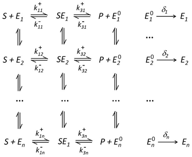
A discrete schematic illustrating the Markovian kinetics of a single enzyme molecule with conformational fluctuations.

In Fig. 2 E₁, E₂, … represent the different conformations of the enzyme, and SE_i are the different conformations of the enzyme-substrate complex. The model is based on the insight that a protein molecule can have multiple conformational states: these states have different atomic arrangements and can have different biochemical functional activities. Detailed calculation in [72, 73, 78, 79] shows that the model is capable of explaining the experimental data.

The data from experiments like [73] have different pattern from the on-off data of [12]. Since fluorescent product is used, which, once formed, quickly diffuses away from the focus of the microscope, the experimental data consist of fluorescent spikes, with each spike corresponding to the formation of one product molecule, amid fluorescence from the background. In principle, the time lag between two successive spikes is the (individual) turnover time of the enzyme. In practice, since the level of the fluorescent spike is random (as a product molecule spends a random time in the focal area of the microscope before diffusing away), one needs to threshold the data to locate the spikes. Finding statistically efficient thresholding level (to minimize false positive) for such data is an open problem.

5.6 Motor protein with mechanical movements against external force

One particular type of enzymes, called motor proteins, can move along their designated linear, periodic tracks inside a living cell, even against a resistant force. The energy of the motor is derived from the chemical potential in the S → P reaction, given in equation (21) [80, 81, 82, 83, 84].

An external mechanical force F_ext enters the rate constants for a conformational transition of a motor protein as follows: If the transition from conformational state A to state B moves a distance d_AB along the track against the force, then according to Boltzmann's law

$$\frac{k_{A\to B}\left(F_{\mathit{\text{ext}}}\right)}{k_{B\to A}\left(F_{\mathit{\text{ext}}}\right)}=\frac{k_{A\to B}(0)}{k_{B\to A}(0)}exp\left(-\frac{F_{\mathit{\text{ext}}}{d}_{\mathit{\text{AB}}}}{k_{B}T}\right).$$

Substituting such a relation into equation (21), and let d be the total motor step length for one enzyme cycle (from S to P), then

$$e_p=J^{\mathit{\text{ness}}}\times \frac{1}{k_{B}T}\left(\mathrm{\Delta }{\mu }_{S\to P}-F_{\mathit{\text{ext}}}d\right).$$

In this case, part of the chemical energy from transformation S → P is converted to mechanical energy. The part that becomes heat is the entropy production.

The motor protein carries out a biased random walk with velocity v_motor = J^nessd. With increasing force F_ext, v_motor decreases. When F_ext = Δμ_S→P/d, the random walk is no longer biased; this is known as a stalling force. One can also compute the dispersion of the motor, i.e., a “diffusion coefficient”:

$$D_{\mathit{\text{motor}}}=\frac{d^2}{2E\left[T_c\right]},E\left[T_c\right]=\frac{1+c_S/K_M+c_P/K_M^P}{\left(V_{\mathit{max}}/K_M\right)c_S+\left(V_{\mathit{max}}^{-}/K_M^P\right)c_P}.$$

In fact, as a semi-Markov process (also known as Markov renewal process or continuous-time random walk), the mean cycle time is E[T_c] and the ratio of probabilities of forward and backward cycles is $\frac{(V_{\mathit{max}}/K_M)c_S}{(V_{\mathit{max}}^{-}/K_M^P)c_P}$.

5.7 Advanced topics

5.7.1 Empirical measure with finite time

Even for the simplest two-state Markov process, some of the statistics can be complex. For example, [85] studies analytically the statistical quantity

$$X_{\tau }=\frac{1}{\tau }{\int }_0^{\tau }{\xi }_B(t)\mathit{\text{dt}}$$

in which ξ_B(t) is the indicator function for state B in Eq. (18). They showed that the pdf (probability density function) of X_τ can be obtained in terms of its Fourier transform γ(y):

$$\gamma (y)=e^{-\frac{1}{2}(k\tau +iy)}\left[cos\mathrm{h}\varphi +\left(\frac{\alpha }{\varphi }\right)sin\mathrm{h}\varphi \right]$$

in which $k=k_1^{+}+k_1^{-},\alpha =\frac{1}{2}k\tau -i\left(p-\frac{1}{2}\right)y,p=k_1^{+}/\left(k_1^{+}+k_1^{-}\right)$, and

$${\varphi }^2={\left(\frac{k\tau }{2}\right)}^2-i\left(p-\frac{1}{2}\right)-{\left(\frac{y}{2}\right)}^2.$$

We see for large τ,

$$\gamma (y)=e^{-\frac{{\sigma }^2(\tau )y^2}{2}-\mathit{\text{ipy}}},{\sigma }^2(\tau )=\frac{2p(1-p)}{k\tau }.$$

5.7.2 Non-Markovian two-state systems

Some enzymes exhibit clear two-state stochastic behavior, but the process is not Markovian. For example, the consecutive dwell times in state B could have non-zero correlation [12]. This is a strong violation of the Markovian property. To explain this observation, the theory of dynamic disorder, or fluctuating enzyme, assumes that $k_1^{+}$ and $k_1^{-}$ in equation (18) are themselves stochastic processes in the form $k_1^{\pm }(t)={\tilde{k}}_1^{\pm }{e}^{-X_t}$ in which X_t is an Ornstein-Uhlenbeck process (see Eq. (3)) [86, 87, 88]. In this case, even though ξ_B(t) is no longer a Markov process, (ξ_B, X) together is now a coupled diffusion process [89]. A more complex model on X_t (describing it as fractional Gaussian noise) is considered in [90]. One can also model X_t by the generalized Langevin equation [91] of Sec. 2.2.

5.7.3 Dwell time distribution peaking

As we have discussed above, a continuous-time Markov chain in a NESS can have complex eigenvalues, thus the power spectrum of its stationary data can exhibit off-zero peak representing intrinsic frequency [92]. However, a surprising result is that one can also observe an off-zero peak in the pdf of the dwell time within a group of states, and this is impossible for a reversible process. This has been discovered independently in [93, 94, 95].

5.7.4 Detailed balance violation and event ordering

The fundamental insight that an sustained chemical energy input is necessary for observing an irreversible Markov process in molecular systems has opened several lines of inquiry on stationary data. On the one hand, for stationary molecular fluctuations in chemico-thermodynamic equilibrium, one wants to test the preservation of detailed balance [96, 97, 98]. On the other hand, for a molecular process with unknown mechanism, one wants to discover whether it is chemically driven [99]. In fact, a quantification of the deviation from reversibility could reveal the source of external energy supply. Finally, for system with breakdown of detailed balance, the event ordering from statistical analysis provides insights toward molecular mechanism [100].

The concept of detailed balance also exists in chemistry [64, 101, 102]. But it is essentially different from the same term known in statistics. The chemical detailed balance requires that a set of linear and nonlinear reactions forming a reaction cycle has zero cycle flux in chemical equilibrium. This chemical detailed-balance is expressed in terms of concentrations of the reactants, which are deterministic quantities. There is no probability involved in this statement. If all the reactions are unimolecular, however, then a chemical reaction system in terms of the law of mass action is equivalent to a continuous-time Markov chain. Only in this case the chemical and the probabilistic detailed balance conditions are the same.

6 Polymer dynamics and Gaussian processes

Polymer dynamics is another highly successful theory based on stochastic processes [103, 104]. A polymer chain in aqueous solution is modelled by a string of identical beads connected by harmonic springs. The Langevin equation for the k^th bead (k = 1, 2, …, N) is

$$m\frac{d^2{X}_k}{{\mathit{\text{dt}}}^2}+\zeta \frac{{\mathit{\text{dX}}}_k}{\mathit{\text{dt}}}=\alpha \left(X_{k-1}-2X_k+X_{k+1}\right)+\sqrt{2\zeta k_{B}T}\frac{{\mathit{\text{dB}}}_k(t)}{\mathit{\text{dt}}},$$ (24)

in which α is the spring constant, m and ζ are the mass and damping coefficient of a bead, and B_k(t) are i.i.d. Wiener processes, again representing the collisions with the solvent. Usually the mechanical system is under overdamped condition, e.g., mα ≪ ζ², in which the acceleration is negligible. Then equation (24) is simplified to

$$\zeta \frac{{\mathit{\text{dX}}}_k}{\mathit{\text{dt}}}=\alpha \left(X_{k-1}-2X_k+X_{k+1}\right)+\sqrt{2\zeta k_{B}T}\frac{{\mathit{\text{dB}}}_k(t)}{\mathit{\text{dt}}}.$$ (25)

This is a multi-dimensional OU process. A polymer molecule presented by such a dynamics is called a Gaussian chain.

One uses the boundary condition X₀(t) = 0 to represent a tethered polymer end, and X_N(t) = X_N+1(t) to represent a free polymer end. To study (25), an elegant approach is to approximate it by a stochastic partial differential equation (SPDE):

$$\zeta \frac{\partial X(s,t)}{\partial t}=\alpha \frac{{\partial }^{2}X(s,t)}{\partial s^2}+\sqrt{2\zeta k_{B}T}\frac{\mathit{\text{dB}}(s,t)}{\mathit{\text{dt}}},$$

in which $\frac{d}{\mathit{\text{dt}}}B(s,t)$ represents a spatio-temporal white noise. With the boundary conditions X(0, t) = 0 and $\frac{\partial X(L,t)}{\partial s}=0$, Fourier transform yields

$$X(s,t)=\sum _{j=0}^{\infty }{\xi }_j(t)sin({\lambda }_{j}s),{\lambda }_j=\left(j+\frac{1}{2}\right)\frac{\pi }{L},$$

in which each normal mode

$$\zeta \frac{d{\xi }_j(t)}{\mathit{\text{dt}}}=-\alpha {\lambda }_j^2{\xi }_j(t)+F_j(t),$$

and

$$E\left[F_i(t)F_j(\tau )\right]=\left(\frac{4\zeta k_{B}T}{L}\right){\delta }_{ij}\delta (t-\tau ).$$

Each ξ_j(t) is an OU process; its stationary distribution has variance

$${\sigma }_j^2=\frac{2k_{B}T}{\alpha {\lambda }_j^{2}L}.$$

Therefore, X(s, t) is a Gaussian random field with stationary variance

$${\sigma }^2(s)=\sum _{j=0}^{\infty }\left(\frac{2k_{B}T}{\alpha {\lambda }_j^{2}L}\right){sin}^2\left({\lambda }_{j}s\right).$$

One strong prediction of the Gaussian polymer theory is that the end-to-end distance of a long polymer should be scaled as the square-root of its molecular weight M. This result has become the standard against which a real polymer is classified: When a polymer is dissolved in a “bad” solvent, its conformation is more collapsed, and thus its end-to-end distance might scale as M^ν with ν < 1/2. On the other hand, due to physical exclusion among polymer segments, a real polymer in a “good” solvent is expected to be more expanded with ν > 1/2. Indeed, the problem of excluded-volume effect in polymer theory has been a major topic in chemistry and in mathematics. Paul Flory received the 1974 Nobel Prize in Chemistry for his studies leading to a ν = 3/4. The rigorous mathematical work on this subject, known as self-avoiding random walks, was carried out by Wendelin Werner, who received 2006 Fields Medal for related work.

6.1 Tethered particle motion measuring DNA looping

Polymer theory has been widely applied in modeling biomacromolecules, especially DNA [105]. In 1990s, Gelles, Sheetz, and their colleagues have developed a single-molecule method to study transcription and DNA looping, called tethered particle motion (TPM) [106, 107]. This time, the trajectory a Brownian motion particle, attached to a piece of DNA, is followed. The statistical movements of the particle, therefore, provide informations on the DNA flexibility, length, etc. The theory for the TPM requires a boundary condition at X_N that is different from Eq. (25), taking into account of the much larger particle that serves as the optical marker [108, 109].

6.2 Rubber elasticity and entropic force

The Gaussian chain theory owes its great success to the Central Limit Theorem (CLT). The end-to-end distance of a polymer chain can be thought as a sum of N i.i.d. random segment l_k, 1 ≤ k ≤ N, where N is proportional to the total molecular weight M. As long as l has a distribution with finite second moment, then [103]

$$E\left[{\Vert \sum _{k=1}^N{\mathbf{l}}_k\Vert }^2\right]=\sum _{j=1}^N\sum _{k=1}^{N}E\left[{\mathbf{l}}_j\cdot {\mathbf{l}}_k\right]=N{\sigma }^2.$$

in which, due to spatial symmetry, it is assumed that E[l_j · l_k] = σ²δ_jk.

We like to point out that the elasticity of rubber is not due to any other molecular interaction, to a large extent, but simply a consequence of this statistical behavior of a Gaussian chain. The end-to-end distance is asymptotically a Gaussian random variable with variance Nσ²:

$$\frac{1}{\sqrt{2\pi N{\sigma }^2}}{e}^{-x^2/(2N{\sigma }^2)}(\text{for large}N).$$

Let one end of a chain be attached. Then the stochastic chain dynamics, on average, pulls the free end from less probable position toward more probable position: This is called “entropic force” in polymer physics. In fact, reversing the Boltzmann's Law, there is an equivalent harmonic “entropy potential energy” U(x) = k_BTx²/(2Nσ²) with springer constant k_BT/(Nσ²).

6.3 Potential of mean force and conditional probability

Stationary probability giving rise to an equivalent “force” is one of the fundamental insights from polymer chemistry. A key concept in statistical chemistry, first developed by John Kirkwood in 1930s [110], is the potential of mean force, which we shall discuss in this subsection. It is essentially an incarnation of the conditional probability.

To illustrate the idea, let us again consider the Langevin equation for an overdamped particle in a potential U(x):

$$\mathit{\text{dX}}(t)=\frac{1}{\zeta }\left(-U^{\prime }(X)\mathit{\text{dt}}+\sqrt{2\zeta k_{B}T}\mathit{\text{dB}}(t)\right).$$

The corresponding Kolmogorov forward equation, for probability density function f_X(x, t) is

$$\frac{\partial f_X(x,t)}{\partial t}=\frac{1}{\zeta }\frac{\partial }{\partial x}\left(k_{B}T\frac{\partial f_X(x,t)}{\partial x}+\frac{\mathit{\text{dU}}(x)}{\mathit{\text{dx}}}{f}_X(x,t)\right),$$ (26)

in which the −U′(x) term represents a potential force acting on the Brownian particle.

Now let us consider a Brownian particle in a 3-dimensional space without any force. If one is only interested in the distance of the Brownian particle to the origin: R(t), then the pdf f_R(r, t) follows a Kolmogorov forward equation:

$$\frac{\partial f_R(r,t)}{\partial t}=\frac{k_{B}T}{\zeta }\frac{\partial }{\partial r}\left(\frac{\partial f_R(r,t)}{\partial t}-\frac{2}{r}{f}_R(r,t)\right).$$ (27)

Comparing equation (27) to (26), we see that the stochastic motion of R(t) experiences an equivalent force 2k_BT/r, with a potential function U_R(r) = −2k_BT ln r. This is again an entropic force, and the corresponding U_R(r) is called potential of mean force. We recognize that the entropic force arises essentially from a change of measure, therefore, it is fundamentally rooted in the theory of probability. The potential of mean force U_R(r) should be understood as

$$U_R(r)=-k_{B}Tln\{\text{conditional stationary prob. given}R=r\}+\text{const}.$$ (28)

Eq. (28) is again applying the Boltzmann's law in reverse, relating an energy to probability.

7 Statistical description of general stochastic dynamics

7.1 Chemical kinetic systems as a paradigm for complex dynamics

It is arguable that, since the work of Kramers, chemists are among the first groups to fully appreciate the nature of separation of time scales in complex dynamics: while the rapid atomic movements in a molecule is extremely fast on the order pico- to femto-seconds, a chemical reaction which involves passing through a saddle point in the energy landscape, on this time scale is a rare event. From this realization, the notions of transition state and reaction coordinate have become two of the most elusive, yet extremely important concepts distinctly chemical. They are even more important in biophysics, which, among others, deals with the transitions between conformational states of proteins. Although not being widely articulated, this is the appropriate statistical treatment of any dynamic system with a separation of time scales due to statistical multi-modality.

7.2 General Markov dynamics with irreversible thermodynamics

Ever since the work of Kolmogorov, reversible, or symmetric Markov process has been widely studied both in theory and in applications. Detailed balance is one of the most important concepts in the theory of MCMC. On the other hand, the notion of entropy has grown increasingly prominent in the general discussions on complex systems, usually in connection to the information theory.

The central role of irreversible Markov description of complex biophysical processes is now firmed established. In recent years, it has also become clear that entropy, and entropy production, are essential concepts in irreversible, often stationary, Markov processes. In this section, we give a concise description of this emergent statistical dynamic theory. We shall only present the key results and leave out all the mathematical proofs, which can be found in the literature [15, 111, 112, 113].

Consider a diffusion process with its Kolmogorov forward equation in the form of

$$\frac{\partial f(x,t)}{\partial t}=\nabla \cdot (D(x)\nabla f(x,t)-b(x)f(x,t))=\mathcal{L}[f].$$ (29)

We assume that it has an ergodic, differentiable stationary density f^ness(x), x ∈ Ω. Then one can define two essential thermodynamic quantities: internal energy of the system U(x) = −ln f^ness(x) and entropy of the entire system

$$S[f(x,t)]=-{\int }_{\mathrm{\Omega }}f(x,t)lnf(x,t)\mathit{\text{dx}}.$$

Then one has the expected value of the U and the so called generalized free energy Ψ [f(x, t)] = E[U] − S:

$$E[U](t)={\int }_{\mathrm{\Omega }}U(x)f(x,t)\mathit{\text{dx}},\Psi [f(x,t)]={\int }_{\mathrm{\Omega }}f(x,t)ln\left(\frac{f(x,t)}{f^{\mathit{\text{ness}}}(x)}\right)\mathit{\text{dx}}.$$ (30)

As a relative entropy, the importance of Ψ ≥ 0 is widely known. Then one has the following set of equations that constitute a theory of irreversible thermodynamics:

$$\frac{d\Psi }{\mathit{\text{dt}}}=E_{\mathit{\text{in}}}-e_p\le 0,\frac{\mathit{\text{dS}}}{\mathit{\text{dt}}}=e_p-h_{\mathit{\text{ex}}},E_{\mathit{\text{in}}},e_p\ge 0;$$ (31a)

$$E_{\mathit{\text{in}}}(t)={\int }_{\mathrm{\Omega }}\left(\nabla ln{f}^{\mathit{\text{ness}}}(x)-D^{-1}(x)b(x)\right)J(x,t)\mathit{\text{dx}};$$ (31b)

$$e_p(t)={\int }_{\mathrm{\Omega }}\left(\nabla lnf(x,t)-D^{-1}(x)b(x)\right)J(x,t)\mathit{\text{dx}};$$ (31c)

$$h_{\mathit{\text{ex}}}(t)={\int }_{\mathrm{\Omega }}b(x)D^{-1}(x)J(x,t)\mathit{\text{dx}};$$ (31d)

$$J(x,t)=b(x)f(x,t)-D(x)\nabla f(x,t).$$ (31e)

The first equation in (31a) can be interpreted as an energy balance equation, with the non-negative E_in and e_p as a source and a sink. e_p is called entropy production. The second equation in (31a) is an entropy balance equation, with heat exchange h_ex can be either positive or negative. dΨ/dt ≤ 0 is the second law of thermodynamics.

For a reversible Markov process, E_in(t) = 0 for all t. Its stationary version has J(x) = 0 for all x and e_p = h_ex = 0. This is know as chemico-thermodynamic equilibrium in biophysics. In general, in a nonequilibrium steady state, ∇ · J^ness = 0 but J^ness ≠ 0.

We now turn our attention to the dynamic equation (29). Its generator is ℒ* = ∇ · D(x) ∇ + b(x) ∇. Introducing inner product

$$(\varphi ,\psi )={\int }_{\mathrm{\Omega }}\varphi (x)\psi (x)f^{\mathit{\text{ness}}}(x)dx,$$

then the linear differential operator ℒ* can be decomposed into ${ℒ}^{\ast }={ℒ}_s^{\ast }+{ℒ}_a^{\ast }$, a symmetric and an anti-symmetric part. Correspondingly, one has the operator in (29), ℒ = ℒ_s + ℒ_a:

$${ℒ}_s[u]=\nabla \cdot \left(D(x)\nabla u(x)-(D(x)\nabla ln{f}^{\mathit{\text{ness}}}(x))u(x)\right),$$ (32a)

$${ℒ}_a[u]=\nabla \cdot \left((D(x)\nabla ln{f}^{\mathit{\text{ness}}}(x)-b(x))u(x)\right).$$ (32b)

In connection to the thermodynamics in (31), a diffusion process with pure ℒ_s has E_in(t) = 0; a process with pure ℒ_a has dΨ/dt = 0 for all t. Noting that the operator in (32b) is actually hyperbolic rather than elliptic: it is a generalization of a conservative, classical Hamiltonian dynamics [113]. Eq. (32a) of course is a generalization of the heat kernel. The generalized Markov dynamics, therefore, unifies the Newtonian conservative and Fourier's dissipative dynamics.

Thermodynamics, and the notions of dissipative and conservative dynamics have been the cornerstone of classical physics. We now see that they emerge from a statistical description of Markov processes. It will be an exciting challenge to the practicing statisticians to apply this new-found stochastic perspective in modeling dynamic data.

How to use these mathematical relations in (31)? We give a speculative example: Consider a stochastic biophysical process X_t in stationarity and assume we know its stationary density f^ness(x). Now one carries out a measurement at time t₀ and observes X_t0 = x₀ ± ∊. Conditioning on this information, the process is no longer stationary; and the system in fact possesses an amount of “chemical energy”, which can be utilized for t > t₀. According to the thermodynamic theory, the amount of energy is Ψ[f(x, t₀)] = – ln (f^ness(x₀)/(2∈)). This result is consistent with information theory. How to calibrate this mathematical result against energy in joules and calories, however, is a challenge.

8 Summary and Outlooks

Biological dynamics are complex. Uncertainty is one of the hallmarks of complex behavior, either in the cause(s) of an occurred event, or in the prediction of its future – modeling and predicting weather is one example. This intuitive sense in fact can be mathematically justifies: Voigt [114] has shown that the generalized free energy Ψ defined in (30) is monotonically decreasing if a dynamics is stochastic with uncertainty in the future, or is deterministic but non-invertable with uncertainty in the past (i.e., many-to-one in discrete time). Ψ is conserved in one-to-one dynamics such as determined by differential equations! In contrast to the deterministic view of classical physics with certainty, quantitative descriptions of biological systems and processes require a statistical perspective [115], as testified in many successful theories and discoveries from population genetics, genomics, and bioinformatics. In the context of single-molecule biophysics, where one zooms in on individual molecules to study their behavior and interactions, one at a time, this stochastic view is ever so fundamental: the random motion of and interaction between molecules in time and space are necessarily described by stochastic processes. We have seen in this review that the basic laws and understanding of statistical mechanics naturally lead to many stochastic processes that govern the behavior of the underlying single-molecule system, but more importantly the understanding and advances in stochastic processes theory motivate new physical and chemical concepts – entropy production in nonequilibrium steady state developed from studying irreversible Markov processes is one such example. The statistical inference of single-molecule experimental data, ranging from exploratory data analysis, testing stochastic models to the estimation of model parameters, has the distinctive feature that the data are typically not the familiar i.i.d. (or independence) type. Often the underlying stochastic-process model does not offer closed-form likelihood; even numerical evaluations are difficult in many models; missing data, in the form of missing components/states or state-aggregation, are prevalent owing to the experimental limitations. There are many open problems in stochastic model building, theoretical investigation of stochastic processes, testing a stochastic model and the estimation of model parameters. The development in stochastic-process theory and the statistical analysis of stochastic-process data will in turn provide new modeling and data-analysis tools for biologists, chemists and physicists. We believe the many open problems present great opportunities for statisticians and probabilists, not only to provide correlations and distributions, but to actually determine mechanistic causality through statistical analysis.

Stochastic process is a more natural language than classical differential equations for chemical and biochemical dynamics at the levels of single molecules and individual cells. It is still not widely appreciated that many of the key notions in chemistry echo important concepts in the theory of probability: transition state as the “origin” of a rare event, chemical potential as a form of stationary probability, Gaussian chain as a consequence of the Central Limit Theorem, and potential of mean force as a manifestation of conditional probability, to name a few. All these chemical concepts have fundamental roots in statistics, though most of them were developed independently by chemists without the explicit usage of modern theory of probability and stochastic processes.

8.1 Mechanism, entropic force and statistics

Before closing, we would like to discuss a philosophical point one inevitably encounters in statistical modeling of complex dynamic data. A fundamental reason to study dynamics in classical sciences is to establish causal relations between events in the sense that modern scientific understanding demands a “mechanism” beyond mere statistical correlations. However, non-deterministic dynamics with random elements raises a very different kind of “understanding”: a force that exerts on a population level might not exist at all on an individuals level; the former is an emergent phenomenon.

Taking the celebrated Fick's law as an example. For a large collection of i.i.d. Brownian particles with diffusion coefficient D, their density flux clearly follows J(x, t) = −D∇c(x, t) where c(x, t) is the concentration of the particle. A net movement of the particle population is due to “more particles moving from a high-concentration region to a low-concentration region than the reverse”, while every particle moves in completely random direction. There is a “Fickean force” pushing the particle population; but this force is not acting on any one individual in the population. Therefore, this Fickean force is a simple example of the concept of entropic force discussed in Sec. 6.2. In fact, noting D = k_BT/ζ, J(x, t) can be expressed as (1/ζ)∇S(x, t) × c(x, t) where S(x, t) = − k_BT ln c(x, t) is a form of energy if one applies the Boltzmann's law in reverse.

This simple example illustrates that in statistical understanding of stochastic dynamics, one needs to be able to appreciate a fundamentally novel type of “law of force” that has no mechanical counterpart. This is the notion of entropy first developed by physicists in thermodynamics. But its significance goes far beyond molecular physics; so is the Second Law that accompanies it. In fact, we believe these concepts are firmly grounded in the domain of probability and statistics. More and deeper investigations are clearly needed.

References

- 1.Perrin JB. Atoms. In: Hammick DL, editor. Eng Trans. D. van Nostrand; New York: 1916. [Google Scholar]
- 2.Wax N, editor. Selected Papers on Noise and Stochastic Processes. Dover; New York: 1954. [Google Scholar]
- 3.Kac M. Lect Appl Math. Vol. 1. Intersci. Pub.; New York: 1959. Probability and Related Topics in Physical Sciences. [Google Scholar]
- 4.Kac M. Enigmas of Chance: An Autobiography. Harper and Row; New York: 1985. [Google Scholar]
- 5.Kramers HA. Brownian motion in a field of force and the diffusion model of chemical reactions. Physica. 1940;7:284–304. [Google Scholar]
- 6.Delbrück M. Statistical fluctuations in autocatalytic reactions. J Chem Phys. 1940;8:120–124. [Google Scholar]
- 7.Schuss Z. Theory and Applications of Stochastic Processes: An Analytical Approach. Springer; New York: 2010. [Google Scholar]
- 8.McQuarrie DA. Stochastic approach to chemical kinetics. J Appl Prob. 1967;4:413–478. [Google Scholar]
- 9.Gillespie DT. Exact stochastic simulation of coupled chemical reactions. J Phys Chem. 1977;81:2340–2361. [Google Scholar]
- 10.Doob JL. Topics in the theory of Markoff chain. Trans Am Math Soc. 1942;52:37–64. [Google Scholar]
- 11.Sakmann B, Neher E, editors. Single-Channel Recording. 2nd. Springer; 2009. 2nd printing. [Google Scholar]
- 12.Lu HP, Xun L, Xie XS. Single molecule enzymatic dynamics. Science. 1998;282:1877–1882. doi: 10.1126/science.282.5395.1877. [DOI] [PubMed] [Google Scholar]
- 13.Chandler D. Introduction to Modern Statistical Mechanics. Oxford University Press; 1987. [Google Scholar]
- 14.Qian H. Mathematical formalism for isothermal linear irreversibility. Proc Roy Soc A. 2001;457:1645–1655. [Google Scholar]
- 15.Qian H, Qian M, Tang X. Thermodynamics of the general diffusion process: Time-reversibility and entropy production. J Stat Phys. 2002;107:1129–1141. [Google Scholar]
- 16.Ruben H. The estimation of a fundamental interaction parameter in an emigration-immigration process. Ann Math Statist. 1963;34:238–259. [Google Scholar]
- 17.McDunnough P. Some aspects of the Smoluchowski process. J Appl Prob. 1978;15:663–674. [Google Scholar]
- 18.Weber SC, Thompson MA, Moerner WE, Spakowitz AJ, Theriot JA. Analytical tools to distinguish the effects of localization error, confinement, and medium elasticity on the velocity autocorrelation function. Biophys J. 2012;102:2443–2450. doi: 10.1016/j.bpj.2012.03.062. [DOI] [PMC free article] [PubMed] [Google Scholar]
- 19.Saxton MJ, Jacobson K. Single-particle tracking: applications to membrane dynamics. Annual Review of Biophysics and Biomolecular Structure. 1997;26:373–399. doi: 10.1146/annurev.biophys.26.1.373. [DOI] [PubMed] [Google Scholar]
- 20.Qian H, Sheetz MP, Elson EL. Single particle tracking. Analysis of diffusion and flow in two-dimensional systems. Biophysical Journal. 1991;60:910–921. doi: 10.1016/S0006-3495(91)82125-7. [DOI] [PMC free article] [PubMed] [Google Scholar]
- 21.Michalet X. Mean square displacement analysis of single-particle trajectories with localization error: Brownian motion in an isotropic medium. Phys Rev E. 2010;82:041914. doi: 10.1103/PhysRevE.82.041914. [DOI] [PMC free article] [PubMed] [Google Scholar]
- 22.Berglund AJ. Statistics of camera-based single-particle tracking. Phys Rev E. 2010;82:011917. doi: 10.1103/PhysRevE.82.011917. [DOI] [PubMed] [Google Scholar]
- 23.Michalet X, Berglund AJ. Optimal diffusion coefficient estimation in single-particle traking. Phys Rev E. 2012;85:061916. doi: 10.1103/PhysRevE.85.061916. [DOI] [PMC free article] [PubMed] [Google Scholar]
- 24.Gloter A, Jacod J. Diffusions with measurement errors. I. Local Asymptotic Normality. ESAIM: Probability and Statistics. 2001;5:225–242. [Google Scholar]
- 25.Gloter A, Jacod J. Diffusions with measurement errors. II. Optimal estimators. ESAIM: Probability and Statistics. 2001;5:243–260. [Google Scholar]
- 26.Cai T, Munk A, Schmidt-Hieber J. Sharp Minimax Estimation of the Variance of Brownian Motion Corrupted with Gaussian Noise. Statistica Sinica. 2010;20:1011–1024. [Google Scholar]
- 27.Blainey PC, Luo G, Kou SC, Mangel WF, Verdine GL, Bagchi B, Xie XS. Nonspecifically bound proteins spin while diffusing along DNA. Nature Structural & Molecular Biology. 2009;16:1224–1229. doi: 10.1038/nsmb.1716. [DOI] [PMC free article] [PubMed] [Google Scholar]
- 28.Halford SE, Marko JF. How do site-specific DNA-binding proteins find their targets? Nucleic Acid Res. 2004;32:3040–3052. doi: 10.1093/nar/gkh624. [DOI] [PMC free article] [PubMed] [Google Scholar]
- 29.Slutsky M, Mirny LA. Kinetics of protein-DNA interaction: facilitated target location in sequence-dependent potential. Biophys J. 2004;87:4021–4035. doi: 10.1529/biophysj.104.050765. [DOI] [PMC free article] [PubMed] [Google Scholar]
- 30.Schurr JM. The one-dimensional diffusion coefficient of proteins absorbed on DNA. Hydrodynamic considerations. Biophys Chem. 1979;9:413–414. [PubMed] [Google Scholar]
- 31.Bagchi B, Blainey P, Xie XS. Diffusion constant of a nonspecifically bound protein undergoing curvilinear motion along DNA. J Phys Chem B. 2008;112:6282–6284. doi: 10.1021/jp077568f. [DOI] [PubMed] [Google Scholar]
- 32.Bouchaud J, Georges A. Anomalous diffusion in disordered media: Statistical mechanisms, models and physical applications. Phys Rep. 1990;195:127–293. [Google Scholar]
- 33.Klafter J, Shlesinger M, Zumofen G. Beyond Brownian Motion. Physics Today. 1996;49:33–39. [Google Scholar]
- 34.Metzler R, Klafter J. The random walk's guide to anomalous diffusion: a fractional dynamics approach. Physics Reports. 2000;339:1–77. [Google Scholar]
- 35.Zwanzig R. Nonequilibrium Statistical Mechanics. Oxford University Press; New York: 2001. [Google Scholar]
- 36.Embrechts P, Maejima M. Self-similar Processes. Princeton University Press; Princeton, New Jersey: 2002. [Google Scholar]
- 37.Qian H. Fractional Brownian motion and fractional Gaussian noise. In: Rangarajan G, Ding MZ, editors. Processes with Long-Range Correlations: Theory and Applications. Vol. 621. Springer; 2003. pp. 22–33. LNP. [Google Scholar]
- 38.Kou SC. Stochastic modeling in nanoscale biophysics: subdiffusion within proteins. Ann Appl Statist. 2008a;2:501–535. [Google Scholar]
- 39.Yang H, Luo G, Karnchanaphanurach P, Louise TM, Rech I, Cova S, Xun L, Xie XS. Protein conformational dynamics probed by single-molecule electron transfer. Science. 2003;302:262–266. doi: 10.1126/science.1086911. [DOI] [PubMed] [Google Scholar]
- 40.Min W, Luo G, Cherayil B, Kou SC, Xie XS. Observation of a power law memory kernel for fluctuations within a single protein molecule. Physical Review Letters. 2005;94:198302(1)–198302(4). doi: 10.1103/PhysRevLett.94.198302. [DOI] [PubMed] [Google Scholar]
- 41.Min W, English B, Luo G, Cherayil B, Kou SC, Xie XS. Fluctuating enzymes: lessons from single-molecule studies. Accounts of Chemical Research. 2005;38:923–931. doi: 10.1021/ar040133f. [DOI] [PubMed] [Google Scholar]
- 42.Ruben H. Generalized concentration fluctuations under diffusion equilibrium. J Appl Prob. 1964;1:47–68. [Google Scholar]
- 43.Brenner SL, Nossal RJ, Weiss GH. Number fluctuation analysis of random locomotion: Statistics of a Smoluchowski process. J Stat Phys. 1978;18:1–18. [Google Scholar]
- 44.Bingham NH, Dunham B. Estimating diffusion coefficients from count data: Einstein-Smoluchowski theory revisited. Ann Inst Statist Math. 1997;49:667–679. [Google Scholar]
- 45.Chandrasekhar S. Stochastic problems in physics and astronomy. Rev Mod Phys. 1943;15:1–89. [Google Scholar]
- 46.Rigler R, Elson EL. Springer Ser Chem Phys. Vol. 65. Springer; New York: 2001. Fluorescence Correlation Spectroscopy: Theory and Applications. [Google Scholar]
- 47.Qian H, Raymond GM, Bassingthwaighte JB. Stochastic fractal behaviour in concentration fluctuation and fluorescence correlation spectroscopy. Biophys Chem. 1999;80:1–5. doi: 10.1016/s0301-4622(99)00031-9. [DOI] [PMC free article] [PubMed] [Google Scholar]
- 48.Wiener N. Nonlinear Problems In Random Theory. The MIT Press; Boston: 1966. [Google Scholar]
- 49.Ridgeway WK, Millar DP, Williamson JR. The spectroscopic basis of fluorescence triple correlation spectroscopy. J Phys Chem. 2012;116:1908–1919. doi: 10.1021/jp208605z. [DOI] [PMC free article] [PubMed] [Google Scholar]
- 50.Qian H. On the statistics of fluorescence correlation spectroscopy. Biophys Chem. 1990;38:49–57. doi: 10.1016/0301-4622(90)80039-a. [DOI] [PubMed] [Google Scholar]
- 51.Schwille P, Meyer-Almes FJ, Rigler R. Fluorescence cross-correlation spectroscopy for multicomponent diffusional analysis in solution. Biophys J. 1997;72:1878–1886. doi: 10.1016/S0006-3495(97)78833-7. [DOI] [PMC free article] [PubMed] [Google Scholar]
- 52.Dertinger T, Pacheco V, von der Hocht I, Hartmann R, Gregor I, Enderlein J. Two-focus fluorescence correlation spectroscopy: A new tool for accurate and absolute diffusion measurements. ChemPhysChem. 2007;8:433–443. doi: 10.1002/cphc.200600638. [DOI] [PubMed] [Google Scholar]
- 53.Reuter GEH. Denumerable Markov processes and the associated contraction semigroups on ℓ. Acta Math. 1957;97:1–46. [Google Scholar]
- 54.Bharucha-Reid AT. Elements of the Theory of Markov Processes and Their Applications. McGraw-Hill; New York: 1960. [Google Scholar]
- 55.Ball FG, Rice JA. Stochastic models for ion channels: Introduction and bibliography. Math Biosci. 1992;112:189–206. doi: 10.1016/0025-5564(92)90023-p. [DOI] [PubMed] [Google Scholar]
- 56.Fredkin DR, Rice JA. On aggregated Markov processes. J Appl Prob. 1986;23:208–214. [Google Scholar]
- 57.Yao YC. Estimating the number of change-points via Schwarz' criterion. Statist Prob Lett. 1988;6:181–189. [Google Scholar]
- 58.Braun JV, Braun RK, Muller HG. Multiple changepoint fitting via quasilikelihood, with application to DNA sequence segmentation. Biometrika. 2000;87:301–314. [Google Scholar]
- 59.Tibshirani R, Saunders M, Rosset S, Zhu J, Knight K. Sparsity and smoothness via the fused lasso. (B).J Roy Statist Soc. 2005;67:91–108. [Google Scholar]
- 60.Hotz T, SchÜtte O, Sieling H, Polupanow T, Diederichsen U, Steinem C, Munk A. Idealizing ion channel recordings by jump segmentation and statistical multiresolution analysis. 2012 doi: 10.1109/TNB.2013.2284063. Preprint. [DOI] [PubMed] [Google Scholar]
- 61.Du C, Kao CL, Kou SC. Stepwise signal extraction via marginal likelihood. 2013 doi: 10.1080/01621459.2015.1006365. Preprint. [DOI] [PMC free article] [PubMed] [Google Scholar]
- 62.Kelly FP. Reversibility and Stochastic Networks. Wiley; Chichester: 1979. Reprinted 1987, 1994. [Google Scholar]
- 63.Wang H, Qian H. On detailed balance and reversibility of semi-Markov processes and single-molecule enzyme kinetics. J Math Phys. 2007;48:013303. [Google Scholar]
- 64.Lewis GN. A new principle of equilibrium. Pror Natl Acad Sci USA. 1925;11:179–183. doi: 10.1073/pnas.11.3.179. [DOI] [PMC free article] [PubMed] [Google Scholar]
- 65.Jiang DQ, Qian M, Qian MP. Lect Notes Math. Vol. 1833. Springer; New York: 2004. Mathematical Theory of Nonequilibrium Steady States. [Google Scholar]
- 66.Zhang XJ, Qian H, Qian M. Stochastic theory of nonequilibrium steady states and its applications (Part I) Phys Rep. 2012;510:1–86. [Google Scholar]
- 67.Ge H, Qian M, Qian H. Stochastic theory of nonequilibrium steady states (Part II): Applications in chemical biophysics. Phys Rep. 2012;510:87–118. [Google Scholar]
- 68.Qian H, Elson EL. Single-molecule enzymology: Stochastic Michaelis-Menten kinetics. Biophys Chem. 2002;101:565–576. doi: 10.1016/s0301-4622(02)00145-x. [DOI] [PubMed] [Google Scholar]
- 69.Qian MP, Qian M, Gong GL. The reversibility and entropy production of Markov processes. Contemp Math. 1991;118:255–261. [Google Scholar]
- 70.Seifert U. Stochastic thermodynamics, fluctuation theorems and molecular machines. Rep Prog Phys. 2012;75:126001. doi: 10.1088/0034-4885/75/12/126001. [DOI] [PubMed] [Google Scholar]
- 71.Kim WH. Ph D dissertation. University of Washington; Seattle, WA: 2011. On the behavior of the entropy production rate of a diffusion process in nonequilibrium steady state. [Google Scholar]
- 72.Kou SC, Cherayil BJ, Min W, English BP, Xie XS. Single-molecule Michaelis-Menten equations. J Phys Chem B. 2005;109:19068–19081. doi: 10.1021/jp051490q. [DOI] [PubMed] [Google Scholar]
- 73.English BP, Min W, van Oijen AM, Lee KT, Luo G, Sun H, Cherayil BJ, Kou SC, Xie XS. Ever-fluctuating single enzyme molecules: Michaelis-Menten equation revisited. Nat Chem Bio. 2006;2:87–94. doi: 10.1038/nchembio759. [DOI] [PubMed] [Google Scholar]
- 74.Qian H. Cooperativity and specificity in enzyme kinetics: A single-molecule time-based perspective. Biophys J. 2008;95:10–17. doi: 10.1529/biophysj.108.131771. mini review. [DOI] [PMC free article] [PubMed] [Google Scholar]
- 75.Min W, Gopich IV, English BP, Kou SC, Xie XS, Szabo A. When does the Michaelis-Menten equation hold for fluctuating enzymes? J Phys Chem B. 2006;110:20093–7. doi: 10.1021/jp065187g. [DOI] [PubMed] [Google Scholar]
- 76.Xie XS, Lu HP. Single-molecule enzymology. J Biol Chem. 1999;274:15967–15970. doi: 10.1074/jbc.274.23.15967. [DOI] [PubMed] [Google Scholar]
- 77.Xie XS. Single molecule approach to enzymology. Single Molecule. 2001;4:229–236. [Google Scholar]
- 78.Kou SC. Stochastic networks in nanoscale biophysics: modeling enzymatic reaction of a single protein. J Amer Statist Assoc. 2008;103:961–975. [Google Scholar]
- 79.Du C, Kou SC. Correlation analysis of enzymatic reaction of a single protein molecule. Annals of Applied Statistics. 2012;6:950–976. doi: 10.1214/12-AOAS541. [DOI] [PMC free article] [PubMed] [Google Scholar]
- 80.Qian H. A simple theory of motor protein kinetics and energetics. Biophys Chem. 1997;67:263–267. doi: 10.1016/s0301-4622(97)00051-3. [DOI] [PubMed] [Google Scholar]
- 81.Fisher ME, Kolomeisky AB. The force exerted by a molecular motor. Proc Natl Acad Sci USA. 1999;96:6597–6602. doi: 10.1073/pnas.96.12.6597. [DOI] [PMC free article] [PubMed] [Google Scholar]
- 82.Qian H. Cycle kinetics, steady-state thermodynamics and motors — a paradigm for living matter physics. J Phys Cond Matt. 2005;17:S3783–S3794. doi: 10.1088/0953-8984/17/47/010. [DOI] [PubMed] [Google Scholar]
- 83.Kolomeisky AB, Fisher ME. Molecular motors: A theorist's perspective. Ann Rev Phys Chem. 2007;58:675–695. doi: 10.1146/annurev.physchem.58.032806.104532. [DOI] [PubMed] [Google Scholar]
- 84.Chowdhury D. Stochastic mechano-chemical kinetics of molecular motors: A multidisciplinary enterprise from a physicists perspective. Phys Rep. 2013;529:1–197. [Google Scholar]
- 85.Geva E, Skinner JL. Two-state dynamics of single biomolecules in solution. Chem Phys Lett. 1998;288:225–229. [Google Scholar]
- 86.Agmon N, Hopfield JJ. Transient kinetics of chemical reactions with bounded diffusion perpendicular to the reaction coordinate: Intramolecular processes with slow conformational changes. J Chem Phys. 1983;78:6947–6959. [Google Scholar]
- 87.Schenter GK, Lu HP, Xie XS. Statistical analysis and theoretical models of single-molecule enzymatic dynamics. J Phys Chem A. 1999;103:10477–88. [Google Scholar]
- 88.Kou SC, Xie XS, Liu JS. Bayesian analysis of single-molecule experimental data (with discussion) (C).J Roy Statist Soc. 2005;54:469–506. [Google Scholar]
- 89.Qian H. Equations for stochastic macromolecular mechanics of single proteins: Equilibrium fluctuations, transient kinetics and nonequilibrium steady-state. J Phys Chem B. 2002;106:2065–73. [Google Scholar]
- 90.Wang J, Wolynes PG. Intermittency of single molecule reaction dynamics in fluctuating environments. Phys Rev Lett. 1995;74:4317–4320. doi: 10.1103/PhysRevLett.74.4317. [DOI] [PubMed] [Google Scholar]
- 91.Kou SC, Xie XS. Generalized Langevin equation with fractional Gaussian noise: Subdiffusion within a single protein molecule. Phys Rev Lett. 2004;93:180603. doi: 10.1103/PhysRevLett.93.180603. [DOI] [PubMed] [Google Scholar]
- 92.Qian H, Qian M. Pumped biochemical reactions, nonequilibrium circulation, and stochastic resonance. Phys Rev Lett. 2000;84:2271–2274. doi: 10.1103/PhysRevLett.84.2271. [DOI] [PubMed] [Google Scholar]
- 93.Li GP, Qian H. Kinetic timing: A novel mechanism for improving the accuracy of GTPase timers in endosome fusion and other biological processes. Traffic. 2002;3:249–255. doi: 10.1034/j.1600-0854.2002.030402.x. [DOI] [PubMed] [Google Scholar]
- 94.Tu Y. The nonequilibrium mechanism for ultrasensitivity in a biological switch: Sensing by Maxwell's demons. Proc Natl Acad Sci USA. 2008;105:11737–41. doi: 10.1073/pnas.0804641105. [DOI] [PMC free article] [PubMed] [Google Scholar]
- 95.Witkoskie JB, Cao JS. Signatures of detailed balance violations in single molecule blinking sequences. doi: 10.1021/jp061471w. Preprint. [DOI] [PubMed] [Google Scholar]
- 96.Rothberg BS, Magleby KL. Testing for detailed balance (microscopic reversibility) in ion channel gating. Biophys J. 2001;80:3025–3026. doi: 10.1016/S0006-3495(01)76268-6. [DOI] [PMC free article] [PubMed] [Google Scholar]
- 97.Witkoskie JB, Cao JS. Testing for renewal and detailed balance violations in single-molecule blinking processes. J Phys Chem B. 2006;110:19009–19017. doi: 10.1021/jp061471w. [DOI] [PubMed] [Google Scholar]
- 98.Nagy I, Tóth J. Microscopic reversibility or detailed balance in ion channel models. J Math Chem. 2012;50:1179–1199. [Google Scholar]
- 99.Qian H, Elson EL. Fluorescence correlation spectroscopy with high-order and dual-color correlation to probe nonequilibrium steady-states. Proc Natl Acad Sci USA. 2004;101:2828–2833. doi: 10.1073/pnas.0305962101. [DOI] [PMC free article] [PubMed] [Google Scholar]
- 100.Sisan DR, Yarar D, Waterman CM, Urbach JS. Event ordering in live-cell imaging determined from temporal cross-correlation asymmetry. Biophys J. 2010;98:2432–41. doi: 10.1016/j.bpj.2010.02.041. [DOI] [PMC free article] [PubMed] [Google Scholar]
- 101.Feinberg M. Necessary and sufficient conditions for detailed balancing in mass action systems of arbitrary complexity. Chem Engr Sci. 1989;44:1819–1827. [Google Scholar]
- 102.Fowler RH, Milne EA. A note on the principle of detailed balancing. Proc Natl Acad Sci USA. 1925;11:400–402. doi: 10.1073/pnas.11.7.400. [DOI] [PMC free article] [PubMed] [Google Scholar]
- 103.Flory PJ. Statistical Mechanics of Chain Molecules. Wiley Interscience; New York: 1969. [Google Scholar]
- 104.Doi M, Edwards SF. The Theory of Polymer Dynamics. Oxford Univ. Press; U.K.: 1988. [Google Scholar]
- 105.Schellman JA. The flexibility of DNA: I. Thermal fluctuations. Biophys Chem. 1980;11:321–328. doi: 10.1016/0301-4622(80)87004-9. [DOI] [PubMed] [Google Scholar]
- 106.Schafer DA, Gelles J, Sheetz MP, Landick R. Transcription by single molecules of RNA polymerase observed by light microscopy. Nature. 1991;352:444–448. doi: 10.1038/352444a0. [DOI] [PubMed] [Google Scholar]
- 107.Finzi L, Gelles J. Measurement of lactose repressor-mediated loop formation and breakdown in single DNA molecules. Science. 1995;267:378–380. doi: 10.1126/science.7824935. [DOI] [PubMed] [Google Scholar]
- 108.Qian H, Elson EL. Quantitative study of polymer conformation and dynamics by single-particle tracking. Biophys J. 1999;76:1598–1605. doi: 10.1016/S0006-3495(99)77319-4. [DOI] [PMC free article] [PubMed] [Google Scholar]
- 109.Qian H. A mathematical analysis of the Brownian dynamics of DNA tether. J Math Biol. 2000;41:331–340. doi: 10.1007/s002850000055. [DOI] [PubMed] [Google Scholar]
- 110.Kirkwood JG. Statistical mechanics of fluid mixtures. J Chem Phys. 1935;3:300–313. 1935. [Google Scholar]
- 111.Ge H, Qian H. The physical origins of entropy production, free energy dissipation and their mathematical representations. Phys Rev E. 2010;81:051133. doi: 10.1103/PhysRevE.81.051133. [DOI] [PubMed] [Google Scholar]
- 112.Esposito M, van den Broeck C. Three detailed fluctuation theorems. Phys Rev Lett. 2010;104:090601. doi: 10.1103/PhysRevLett.104.090601. [DOI] [PubMed] [Google Scholar]
- 113.Qian H. A decomposition of irreversible diffusion processes without detailed balance. J Math Phys. 2013;54:053302. [Google Scholar]
- 114.Voigt J. Stochastic operators, information, and entropy. Commun Math Phys. 1981;81:31–38. [Google Scholar]
- 115.Qian H. Stochastic physics, complex systems and biology. Quant Biol. 2013;1:50–53. [Google Scholar]