Graph Estimation with Joint Additive Models

Abstract

In recent years, there has been considerable interest in estimating conditional independence graphs in high dimensions. Most previous work has assumed that the variables are multivariate Gaussian, or that the conditional means of the variables are linear; in fact, these two assumptions are nearly equivalent. Unfortunately, if these assumptions are violated, the resulting conditional independence estimates can be inaccurate. We propose a semi-parametric method, graph estimation with joint additive models, which allows the conditional means of the features to take on an arbitrary additive form. We present an efficient algorithm for our estimator's computation, and prove that it is consistent. We extend our method to estimation of directed graphs with known causal ordering. Using simulated data, we show that our method performs better than existing methods when there are non-linear relationships among the features, and is comparable to methods that assume multivariate normality when the conditional means are linear. We illustrate our method on a cell-signaling data set.

1. Introduction

In recent years, there has been considerable interest in developing methods to estimate the joint pattern of association within a set of random variables. The relationships between d random variables can be summarized with an undirected graph Γ = (V, S) in which the random variables are represented by the vertices V = {1, . . . , d} and the conditional dependencies between pairs of variables are represented by edges S ⊂ V × V . That is, for each j ∈ V , we want to determine a minimal set of variables on which the conditional densities p_j({X_j | {X_k, k ≠ j}) depend,

$$p_j(X_j\mid \{X_k,k\ne j\})=p_j(X_j\mid \{X_k:(k,j)\in S\}).$$

There has also been considerable work in estimating marginal associations between a set of random variables (see e.g. Basso et al., 2005; Meyer et al., 2008; Liang & Wang, 2008; Hausser & Strimmer, 2009; Chen et al., 2010). But in this paper we focus on conditional dependencies, which, unlike marginal dependencies, cannot be explained by the other variables measured.

Estimating the conditional independence graph Γ based on a set of n observations is an old problem (Dempster, 1972). In the case of high-dimensional continuous data, most previous work has assumed either multivariate Gaussianity (see e.g. Friedman et al., 2008; Rothman et al., 2008; Yuan & Lin, 2007; Banerjee et al., 2008) or linear conditional means (see e.g. Meinshausen & Bühlmann, 2006; Peng et al., 2009) for the features. However, as we will see, these two assumptions are essentially equivalent. Some recently proposed methods relax the multivariate Gaussian assumption using univariate transformations (Liu et al., 2009, 2012; Xue & Zou, 2012; Dobra & Lenkoski, 2011), restrictions on the graph structure (Liu et al., 2011), or flexible random forests (Fellinghauer et al., 2013). However, we will see that these methods may not capture realistic departures from multivariate Gaussianity.

For illustration, consider the cell signaling data set from Sachs et al. (2005), which consists of protein concentrations measured under a set of perturbations. We analyze the data in more detail in Section 5·3. Pairwise scatterplots of three of the variables are given in Fig. 1 (a)-(c) for one of 14 experiments. The data have been transformed to be marginally normal, as suggested by Liu et al. (2009), but the transformed data clearly are not multivariate normal, as confirmed by a Shapiro–Wilk test, which yields a p-value less than 2 × 10⁻¹⁶.

Fig. 1.

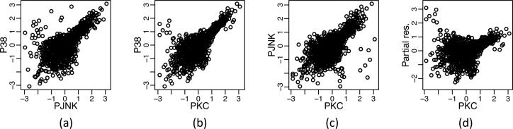
Cell signaling data from Sachs et al. (2005). (a)–(c) Pairwise scatterplots for PKC, P38 and PJNK. (d) Partial residuals from the linear regression of P38 on PKC and PJNK. The data are transformed to have normal marginal distributions, but are clearly not multivariate normal.

Can the data in Fig. 1 be well-represented by linear relationships? In Fig. 1 (d), we see strong evidence that the conditional mean of the protein P38 given PKC and PJNK is nonlinear. This is corroborated by the fact that the p-value for including quadratic terms in the linear regression of P38 onto PKC and PJNK is less than 2 × 10⁻¹⁶. Therefore in this data set, the features are not multivariate Gaussian, and marginal transformations do not remedy the problem.

In order to model this type of data, we could specify a more flexible joint distribution. How-ever, joint distributions are difficult to construct and computationally challenging to fit, and the resulting conditional models need not be easy to obtain or interpret. Alternatively, we can specify the conditional distributions directly; this has the advantage of simpler interpretation and greater computational tractability. In this paper, we will model the conditional means of non-Gaussian random variables with generalized additive models (Hastie & Tibshirani, 1990), and will use these in order to construct conditional independence graphs.

Throughout this paper, we will assume that we are given n independent and identically distributed observations from a d-dimensional random vector $X=(X_1,\dots ,X_d)\sim \mathcal{P}$. Our observed data can be written as $x=(x_1,\dots ,x_d)\in {\mathbb{R}}^{n\times d}$.

2. MODELING CONDITIONAL DEPENDENCE RELATIONSHIPS

Suppose we are interested in estimating the conditional independence graph for a random Γ vector $X\in {\mathbb{R}}^d$. If the joint distribution is known up to some parameter θ, it suffices to estimate θ via e.g. maximum likelihood. One practical difficulty is specification of a plausible joint distribution. Specifying a conditional distribution, such as in a regression model, is typically much less daunting. We therefore consider pseudo-likelihoods (Besag, 1974, 1975) of the form

$$\log \left\{p_{PL}(x;\theta )\right\}=\sum _{j=1}^d\log \left\{p_j(x_j\mid \{x_k:(j,k)\in S\};\theta )\right\}.$$

For a set of arbitrary conditional distributions, there need not be a compatible joint distribution (Wang & Ip, 2008). However, the conditionally specified graphical model has an appealing the-oretical justification, in that it minimizes the Kullback–Leibler distances to the conditional distributions (Varin & Vidoni, 2005). Furthermore, in estimating conditional independence graphs, our scientific interest is in the conditional independence relationships rather than in the joint distribution. So in a sense, modeling the conditional distribution rather than the joint distribution is a more direct approach to graph estimation. We therefore advocate an approach for non-Gaussian graphical modeling based on conditionally specified models (Varin et al., 2011).

3. PREVIOUS WORK

3·1. Estimating graphs with Gaussian data

Suppose for now that X has a joint Gaussian distribution with mean 0 and precision matrix Θ. The negative log-likelihood function evaluated at Θ, up to constants, is

$$-\log \det \left(ϴ\right)+\mathrm{tr}\left(x^{T}xϴ\right)∕n.$$ (1)

In this case, the conditional relationships are linear,

$$X_j\mid \{X_k,k\ne j\}=\sum _{k\ne j}{\beta }_{jk}{X}_k+{∊}_j(j=1,\dots ,d),$$ (2)

where β_jk = −Θ_jk/ Θ_kk and ∈_j ~ N₁(0, 1/Θ_jj). To estimate the graph Γ, we must determine which β_jk are zero in (2), or equivalently, which Θ_jk are 0 in (1). This is simple when n > > d.

In the high-dimensional setting, when the maximum likelihood estimate is unstable or undefined, a number of approaches to estimate the conditional independence graph Γ have been proposed. Meinshausen & Bühlmann (2006) proposed fitting (2) using an l₁-penalized regression. This is referred to as neighborhood selection:

$$\{{\widehat{\beta }}_{jk}:1\le j,k\le d\}=\underset{{\beta }_{jk}:1\le j,k\le d}{\arg \min }\left\{\frac{1}{2}\sum _{j=1}^d{\Vert x_j-\sum _{k\ne j}{x}_k{\beta }_{jk}\Vert }^2+\lambda \sum _{j=1}\sum _{k\ne j}\mid {\beta }_{jk}\mid \right\}.$$ (3)

Here λ is a nonnegative tuning parameter that encourages sparsity in the coefficient estimates. Peng et al. (2009) improved upon the neighborhood selection approach by applying l₁ penalties to the partial correlations; this is known as sparse partial correlation estimation.

As an alternative to (3), many authors have considered estimating Θ by maximizing an l₁-penalized joint log likelihood (see e.g. Yuan & Lin, 2007; Banerjee et al., 2008; Friedman et al., 2008). This amounts to the optimization problem

$$\widehat{ϴ}=\underset{W\succ 0}{\arg \min }\{-\log \det \left(W\right)+\mathrm{tr}\left(x^{T}xW\right)∕n+\lambda {\Vert W\Vert }_1\},$$ (4)

known as the graphical lasso. Here, $W\succ 0$ 0 indicates that W must be positive definite. The sparsity pattern of the solution $\widehat{ϴ}$ to (4) serves as an estimate of Γ.

At first glance, neighborhood selection and sparse partial correlation estimation may seem semi-parametric: a linear model may hold in the absence of multivariate normality. However, while (2) can accurately model each conditional dependence relationship semi-parametrically, the accumulation of these specifications sharply restricts the joint distribution: Khatri & Rao (1976) proved that if (2) holds, along with some mild assumptions, then the joint distribution must be multivariate normal, regardless of the distribution of the errors ε_j in (2). In other words, even though (3) does not explicitly involve the multivariate normal likelihood, normality is implicitly assumed. Thus, if we wish to model non-normal data, non-linear conditional models are necessary.

3·2. Estimating graphs with non-Gaussian data

We now briefly review three existing methods for modeling conditional independence graphs with non-Gaussian data. The normal copula or nonparanormal model (Liu et al. 2009, Liu et al. 2012, Xue & Zou 2012, studied in the Bayesian context by Dobra & Lenkoski 2011) assumes that X has a nonparanormal distribution: that is, {h₁(X₁), . . . , h_d(X_d)} ~ N_d(0, Θ) for monotone functions h₁, . . . , h_d. After these are estimated, one can apply any of the methods mentioned in Section 3·1 to the transformed data. The conditional model implicit in this approach is

$$h_j\left(X_j\right)\mid \{X_k,k\ne j\}=\sum _{k\ne j}{\beta }_{jk}{h}_k\left(X_k\right)+{∊}_j(j=1,\dots ,d).$$ (5)

This restrictive assumption may not hold, as seen in Fig. 1.

Forest density estimation (Liu et al., 2011) replaces the need for distributional assumptions with graphical assumptions: the underlying graph is assumed to be a forest, and bivariate densities are estimated non-parametrically. Unfortunately, the restriction to acyclic graphs may be inappropriate in applications, and maximizing over all possible forests is infeasible.

The graphical random forests (Fellinghauer et al., 2013) approach uses random forests to flexibly model conditional means, and allows for interaction terms. However, random forests do not correspond to a well-defined statistical model or optimization problem, and results on its feature selection consistency are in general unavailable. In contrast, our proposed method corresponds to a statistical model for which we can prove results on edge selection consistency.

4. METHOD

4·1. Jointly additive models

In order to estimate a conditional independence graph using pseudolikelihood, we must estimate the variables on which the conditional distributions p_j (·) depend. However, since density estimation is generally a challenging task, especially in high dimensions, we focus on the simpler problem of estimating the conditional mean E_xj (X_j | {X_k: (j, k) ∈ S} ), under the assumption that the conditional distribution and the conditional mean depend on the same set of variables. Thus, we seek to estimate the conditional mean f_j(·) in the regression model X_j | {X_k, k ≠ j} = f_j (X_k, k ≠ j) + ∈_j) + ∈_j where ∈_j is a mean-zero error term. Since estimating arbitrary functions f_j(·) is infeasible in high dimensions, we restrict ourselves to additive models

$$X_j\mid \{X_k,k\ne j\}=\sum _{k\ne j}{f}_{jk}\left(X_k\right)+{∊}_j,$$ (6)

where f_jk(·) lies in some space of functions $\mathcal{F}$. This amounts to modeling each variable using a generalized additive model (Hastie & Tibshirani, 1990). Unlike Fellinghauer et al. (2013), we do not assume that the errors ∈_j are independent of the additive components f_jk(·), but merely that the conditional independence structure can be recovered from the functions f_jk(·).

4·2. Estimation

Since we believe that the conditional independence graph is sparse, we fit (6) using a penalty that performs simultaneous estimation and selection of the f_jk(·). Specifically, we link together d sparse additive models (Ravikumar et al., 2009) using a penalty that groups the parameters corresponding to a single edge in the graph. This results in the problem

$$\underset{f_{jk}\in \mathcal{F},1\le j,k\le d}{\mathrm{minimize}}\left[\frac{1}{2n}\sum _{j=1}^d{\Vert x_j-\sum _{k\ne j}{f}_{jk}\left(x_k\right)\Vert }_2^2+\lambda \sum _{k>j}{\{{\Vert f_{jk}\left(x_k\right)\Vert }_2^2+{\Vert f_{kj}\left(x_j\right)\Vert }_2^2\}}^{1∕2}\right].$$ (7)

We consider f_jk(x_k) = Ψ_jkβ_jk, where Ψ_jk is a n × r matrix whose columns are basis functions used to model the additive components f_jk, and β_jk is an r-vector containing the associated coefficients. For instance, if we use a linear basis function, Ψ_jk = x_k, then r = 1 and we model only linear conditional means, as in Meinshausen & Bühlmann (2006). Higher-order terms allow us to model more complex dependencies. The standardized group lasso penalty (Simon & Tibshirani, 2012) encourages sparsity and ensures that the estimates of f_jk(·) and f_kj(·) will be simultaneously zero or non-zero. Problem (7) is an extension of sparse additive modeling (Ravikumar et al., 2009) to graphs, and generalizes neighborhood selection (Meinshausen & Bühlmann, 2006) and sparse partial correlation (Peng et al., 2009) to allow for flexible conditional means.

Algorithm 1. Given initial values for the ${\widehat{\beta }}_{jk}$, perform Steps 1–3 for (j, k) ∈ V × V, and repeat until convergence.

Step 1. Calculate the vector of errors for the jth and kth variables:

$$r_{jk}\leftarrow x_j-\sum _{i\ne j,k}{\Psi }_{ji}{\widehat{\beta }}_{ji},r_{kj}\leftarrow x_k-\sum _{i\ne j,k}{\Psi }_{ki}{\widehat{\beta }}_{ki}.$$

Step 2. Regress the errors on the specified basis functions:

$${\widehat{\beta }}_{jk}\leftarrow {\left({\Psi }_{jk}^T{\Psi }_{jk}^{}\right)}^{-1}{\Psi }_{jk}^T{r}_{jk},{\widehat{\beta }}_{kj}\leftarrow {\left({\Psi }_{kj}^T{\Psi }_{kj}\right)}^{-1}{\Psi }_{kj}^T{r}_{jk}.$$

Step 3. Threshold:

$$\begin{array}{cc}\hfill & {\widehat{\beta }}_{jk}\leftarrow {\left\{1-n\lambda {\left({\Vert {\Psi }_{jk}{\widehat{\beta }}_{jk}\Vert }_2^2+{\Vert {\Psi }_{kj}{\widehat{\beta }}_{kj}\Vert }_2^2\right)}^{-1∕2}\right\}}_{+}{\widehat{\beta }}_{jk},\hfill \\ \hfill & {\widehat{\beta }}_{kj}\leftarrow {\left\{1-n\lambda {\left({\Vert {\Psi }_{jk}{\widehat{\beta }}_{jk}\Vert }_2^2+{\Vert {\Psi }_{kj}{\widehat{\beta }}_{kj}\Vert }_2^2\right)}^{-1∕2}\right\}}_{+}{\widehat{\beta }}_{kj}.\hfill \end{array}$$

Algorithm 1 uses block coordinate descent to achieve the global minimum of the convex problem (7) (Tseng, 2001). Performing Step 2 requires an r × r matrix inversion; this must be performed only twice per pair of variables. Estimating 30 conditional independence graphs with r = 3 on a simulated data set with n = 50 and d = 100 takes 1.1 seconds on a 2.8 GHz Intel Core i7 Macbook Pro. The R package spacejam, available at cran.r-project.org/package=spacejam, implements the proposed approach.

4·3. Tuning

A number of options for tuning parameter selection are available, such as generalized crossvalidation (Tibshirani, 1996), the Bayesian information criterion (Zou et al., 2007), and stability selection (Meinshausen & Bühlmann, 2010). We take an approach motivated by the Bayesian information criterion, as in Peng et al. (2009). For the jth variable, the criterion is

$${\mathrm{BIC}}_j\left(\lambda \right)=n\log \left({\Vert x_j-\sum _{k\ne j}{\Psi }_{jk}{\widehat{\beta }}_{jk}^{\left(\lambda \right)}\Vert }_2^2\right)+\log \left(n\right){\mathrm{DF}}_j\left(\lambda \right),$$ (8)

where DF_j(λ) is the degrees of freedom used in this regression. We seek the value of λ that minimizes ${\sum }_{j=1}^d{\mathrm{BIC}}_j\left(\lambda \right)$. When a single basis function is used, we can approximate the degrees of freedom by the number of non-zero parameters in the regression (Zou et al., 2007; Peng et al., 2009). But with r > 1 basis functions, we use

$${\mathrm{DF}}_j\left(\lambda \right)=\mid S_j^{\left(\lambda \right)}\mid +(r-1)\sum _k\frac{{\Vert {\Psi }_{jk}{\widehat{\beta }}_{jk}^{\left(\lambda \right)}\Vert }_2^2}{{\Vert {\Psi }_{jk}{\widehat{\beta }}_{jk}^{\left(\lambda \right)}\Vert }_2^2+\lambda },$$ (9)

where $S_j^{\left(\lambda \right)}=\{k:\Vert {\widehat{\beta }}_{jk}^{\left(\lambda \right)}\Vert \ne 0\}$. Although (9) was derived under the assumption of an orthogonal design matrix, it is a good approximation for the non-orthogonal case (Yuan & Lin, 2006). Chen & Chen (2008) proposed modifications of the Bayesian information criterion for high-dimensional regression, which Gao & Song (2010) extended to the psuedo-likelihood setting. We leave evaluation of these alternatives for future work.

In order to perform Algorithm 1, we must select a set of basis functions. Domain knowledge or experience with similar data may guide basis choice. In the absence of domain knowledge we use cubic polynomials, which can approximate a wide range of functions. In Section 5·1, we use several different bases, and find that even misspecified sets of functions can provide more accurate graph estimates than methods that assume linearity.

5. NUMERICAL EXPERIMENTS

5·1. Simulation setup

As discussed in Section 2, it can be difficult to specify flexible non-Gaussian distributions for continuous variables. However, construction of multivariate distributions via conditional distributions is straightforward when the variables can be represented with a directed acyclic graph. The distribution of variables in a directed acyclic graph can be decomposed as $p(x_1,\dots ,x_d)={\prod }_{j=1}^d{p}_j(x_j\mid \{x_k:(k,j)\in S_D\})$, where S_D denotes the directed edge set of the graph. This is a valid joint distribution regardless of the choice of conditional distributions p_j(x_j | {x_k : (k, j) ∈ S_D) (Pearl, 2000, Chapter 1.4). We chose structural equations of the form

$$X_j\mid \{X_k:(k,j)\in S_D\}=\sum _{(k,j)\in S_D}{f}_{jk}\left(X_k\right)+{∊}_j,$$ (10)

with ∈_j ~ N(0, 1). If the f_jk are chosen to be linear, then the data are multivariate normal, and if the f_jk are non-linear, then the data will typically not correspond to a well-known multivariate distribution. We moralized the directed graph in order to obtain the conditional independence graph (Cowell et al., 2007, Chapter 3.2). Here we have used directed acyclic graphs simply as a tool to generate non-Gaussian data; the full conditional distributions of the random variables created using this approach are not necessarily additive.

We first generated a directed acyclic graph with d = 100 nodes and 80 edges chosen at random from the 4950 possible edges. We used two schemes to construct a distribution on this graph. In the first setting, we chose $f_{jk}\left(x_k\right)=b_{jk1}{x}_k+b_{jk2}{x}_k^2+b_{jk3}{x}_k^3$, where the b_jk1, b_jk2, and b_jk3 are independent and normally distributed with mean zero and variance 1, 0.5, and 0.5, respectively. In the second case, we chose f_jk(x_k) = x_k, resulting in multivariate normal data. In both cases, we scaled the f_jk(x_k) to have unit variance, and generated n = 50 observations. We compared our method to sparse partial correlation (Peng et al., 2009, R package space), graphical lasso (Yuan & Lin, 2007, R package glasso), neighborhood selection (Meinshausen & Bühlmann, 2006, R package glasso), nonparanormal (Liu et al., 2012, R package huge), forest density estimation (Liu et al., 2011, code provided by authors), the method of Basso et al. (2005, R package minet), and graphical random forests (Fellinghauer et al., 2013, code provided by authors). In performing neighborhood selection, we declared an edge between the jth and kth variables if ${\widehat{\beta }}_{jk}\ne 0$ or ${\widehat{\beta }}_{kj}\ne 0$. We performed our method using three sets of basis functions: ${\Psi }_{jk}=(x_k,x_k^2)$, ${\Psi }_{jk}=(x_k,x_k^3)$, ${\Psi }_{jk}=(x_k,x_k^2,x_k^3)$.

5·2. Simulation results

Figure 2 summarizes the results of our simulations. For each method, the numbers of correctly and incorrectly estimated edges were averaged over 100 simulated data sets for a range of 100 tuning parameter values. When the f_jk(·) are non-linear, our method with the basis ${\Psi }_{jk}=(x_k,x_k^2,x_k^3)$ dominates the basis sets ${\Psi }_{jk}=(x_k,x_k^2)$ or $(x_k,x_k^3)$, which in turn tend to enjoy superior performance relative to all other methods, as seen in Fig. 2 (a). Furthermore, even though the basis sets ${\Psi }_{jk}=(x_k,x_k^2)$ and $(x_k,x_k^3)$ do not entirely capture the functional forms of the data-generating mechanism, they still outperform methods that assume linearity, as well as competitors intended to model non-linear relationships.

Fig. 2.

Summary of simulation study. The number of correctly estimated edges is displayed as a function of incorrectly estimated edges, for a range of tuning parameter values, in the (a) non-linear and (b) Gaussian set-ups, averaged over 100 simulated data sets. Dots indicate the average model size chosen by minimizing BIC(λ). The lines display our method with ${\Psi }_{jk}=(x_k,x_k^2)$, (), ${\Psi }_{jk}=(x_k,x_k^3)$ (), and ${\Psi }_{jk}=(x_k,x_k^2,x_k^3)$ (), as well as the methods of Liu et al. (2012)(), Basso et al. (2005) (), Liu et al. (2011) (), Fellinghauer et al. (2013) (), Yuan & Lin (2007) (), Meinshausen & Bühlmann (2006) (), and Peng et al. (2009) ().

When the conditional means are linear and the number of estimated edges is small, all methods perform roughly equally, as seen in Fig. 2 (b). As the number of estimated edges increases, sparse partial correlation performs best, while the graphical lasso, the nonparanormal and the forest-based methods perform worse. This agrees with the observations of Peng et al. (2009) that sparse partial correlation and neighborhood selection tend to outperform the graphical lasso. In this setting, since non-linear terms are not needed to model the conditional dependence relationships, sparse partial correlation outperforms our method with two basis functions, which performs better than our method with three basis functions. Nonetheless, the loss in accuracy due to the inclusion of non-linear basis functions is not dramatic, and our method still tends to outperform other methods for non-Gaussian data, as well as the graphical lasso.

5·3. Application to cell signaling data

We apply our method to a data set consisting of measurements for 11 proteins involved in cell signaling, under 14 different perturbations (Sachs et al., 2005). To begin, we consider data from one of the 14 perturbations with n = 911, and compare our method using cubic polynomials to neighborhood selection, the nonparanormal, and graphical random forests with stability selection. Minimizing BIC(λ) for our method yields a graph with 16 edges. We compare our method to competing methods, selecting tuning parameters such that each graph estimate contains 16 edges, as well as 10 and 20 edges, for the sake of comparison. Figure 3 displays the estimated graphs, along with the directed graph presented in Sachs et al. (2005).

Fig. 3.

Cell signaling data set; graph reported in Sachs et al. (2005) is shown on the left. On the right, graphs were estimated using data from one perturbation of the data set. From top to bottom, panels contain graphs with 20, 16 and 10 edges. From left to right, comparisons are to Peng et al. (2009); Liu et al. (2012); Fellinghauer et al. (2013). We cannot specify an arbitrary graph size using graphical random forests, so graph sizes for that approach do not match exactly.

The graphs estimated using different methods are qualitatively different. If we treat the directed graph from Sachs et al. (2005) as the ground truth, then our method with 16 edges correctly identifies 12 of the edges, compared to 11, 9, and 8 using sparse partial correlation, the nonparanormal, and graphical random forests, respectively.

Next, we examined the other 13 perturbations, and found that for graphs with 16 edges, our method chooses on average 0.93, 0.64 and 0.2 more correct edges than sparse partial correlation, nonparanormal, and graphical random forests, respectively, yielding p = 0.001, 0.19 and 0.68 using the paired t-test. Since graphical random forests does not permit arbitrary specification of graph size, when graphs with 16 edges could not be obtained, we used the next largest graph, resulting in a larger number of correct edges for their method.

In Section 1, we showed that these data are not well-represented by linear models even after the nonparanormal transformation. The superior performance of our method in this section confirms this observation. The qualitative differences between our method and graphical random forests indicate that the approach taken for modeling non-linearity does affect the results obtained.

6. EXTENSION TO DIRECTED GRAPHS

In certain applications, it can be of interest to estimate the causal relationships underlying a set of features, typically represented as a directed acyclic graph. Though directed acyclic graph estimation is in general NP-hard, it is computationally tractable when a causal ordering is known. In fact, in this case, a modification of neighborhood selection is equivalent to the graphical lasso (Shojaie & Michailidis, 2010b). We extend the penalized likelihood framework of Shojaie & Michailidis (2010b) to non-linear additive models by solving

$$\underset{{\beta }_{jk},2\le j\le p,k\prec j}{\mathrm{minimize}}\left\{\frac{1}{2n}{\Vert x_j-\sum _{k\prec j}{\Psi }_{jk}{\beta }_{jk}\Vert }_2^2+\lambda \sum _{k\prec j}{\Vert {\Psi }_{jk}{\beta }_{jk}\Vert }_2\right\},$$

where $k\prec j$ indicates that k precedes j in the causal ordering. When Ψ_jk = x_k, the model is exactly the penalized Gaussian likelihood approach of Shojaie & Michailidis (2010b).

Figure 4 displays the same simulation scenario as Section 5·1, but with the directed graph estimated using the known causal ordering. Results are compared to the penalized Gaussian likelihood approach of Shojaie & Michailidis (2010b). Our method performs best when the true relationships are non-linear, and performs competitively when the relationships are linear.

Fig. 4.

Summary of the directed acyclic graph simulation. The simulation is exactly as in Section 5·1 and Fig. 2. Again, (a) contains the non-linear simulation and (b) contains the Gaussian simulation. For each method, the number of correctly and incorrectly estimated edges are averaged over 100 simulated data sets, for a range of 100 tuning parameter values. The curves displayed are those of our method with ${\Psi }_{jk}=(x_k,x_k^2)$ (), ${\Psi }_{jk}=(x_k,x_k^3)$ (), and ${\Psi }_{jk}=(x_k,x_k^2,x_k^3)$ (), as well as the method of Shojaie & Michailidis (2010b) ().

7. THEORETICAL RESULTS

In this section, we establish consistency of our method for undirected graphs. Similar results hold for directed graphs, but we omit them due to space considerations. The theoretical development follows the sparsistency results for sparse additive models (Ravikumar et al., 2009).

First, we must define the graph for which our method is consistent. Recall that we have the random vector $X=(X_1,\dots ,X_d)\sim \mathcal{P}$, and $x=(x_1,\dots ,x_d)\in {\mathbb{R}}^{n\times d}$ is a matrix where each row is an independent draw from $\mathcal{P}$. For each (j,k) ∈ V × V consider the orthogonal set of basis functions ψ_jkt(·), $t\in \mathbb{N}$. Define the population level parameters ${\beta }_{jk}^{\ast }\in {\mathbb{R}}^{\infty }$ as

$$\{{\beta }_{jk}^{\ast }:k=1,\dots ,d\}\equiv \underset{{\beta }_{jk}:k=1,\dots ,d}{\arg \min }\left\{E{\mid X_j-\sum _{k\ne j}\sum _{t-1}^{\infty }{\psi }_{jkt}\left(X_k\right){\beta }_{jkt}\mid }^2\right\}(j=1,\dots ,d).$$

Let $S_j=\{k:\Vert {\beta }_{jk}^{\ast }\Vert \ne 0\}$, s_j = |S_j|, and $f_{jk}={\sum }_{t=1}^{\infty }{\psi }_{jkt}{\beta }_{jkt}^{\ast }\in \mathcal{F}$. Then

$$X_j=\sum _{k\in S_j}{f}_{jk}\left(X_k\right)+{∊}_j(j=1,\dots ,d),$$

where ∈₁, . . . , ∈_d are errors, and Σ_k∈Sjf_jk(X_k) is the best additive approximation to E(X_j | X_k : k ≠ j), in the least-squares sense. We wish to determine which of the f_jk(·) are zero.

On observed data, we use a finite set of basis functions to model the f_jk(·). Denote the set of r orthogonal basis functions used in the regression of x_j on x_k by Ψ_jk = {ψ_jk1(x_k),..., ψ_jkr(x_k)}, a matrix of dimension n × r such that ${\Psi }_{jk}^T{\Psi }_{jk}∕n=I_r$. Let ${\beta }_{jk}^{\ast \left(r\right)}={({\beta }_{jk1}^{\ast },\dots ,{\beta }_{jkr}^{\ast })}^T$ denote the first r components of ${\beta }_{jk}^{\ast }$. Further, let ${\Psi }_{S_j}\in {\mathbb{R}}^{n\times s_{j}r}$ be the concatenated basis functions in {Ψ_jk : k ∈ S_j} and β_Sj be the corresponding coefficients. Also let ${\Sigma }_{S_j,S_j}=n^{-1}{\Psi }_{S_j}^T{\Psi }_{S_j}$, ${\Sigma }_{jk,S_j}=n^{-1}{\Psi }_{jk}^T{\Psi }_{S_j}$, and ${\Lambda }_{\min }\left({\Sigma }_{S_j,S_j}\right)$, and Λ_min(Σ_Sj,_Sj) be the minimum eigenvalue of Σ_Sj,_Sj. Define the subgradient of the penalty in (7) with respect to β_jk as g_jk(β). On the set S_j, we write the concatenated subgradients as gS_j, a vector of length s_jr.

Let $\widehat{\beta }$ be the parameter estimates from solving (7), let ${\widehat{S}}_n=\{(j,k):{\Vert {\widehat{\beta }}_{jk}\Vert }_2^2+{\Vert {\widehat{\beta }}_{kj}\Vert }_2^2\ne 0\}$ be the corresponding estimated edge set, and let S* = {(j,k) : k ∈ S_j or j ∈ S_k} be the graph obtained from the population level parameters. In Theorem 1, proved in the Appendix, we give precise conditions under which $\mathrm{pr}({\widehat{S}}_n=S^{\ast })\to 1$ as n → ∞.

THEOREM 1. Let the functions f_jk be sufficently smooth, in thesense that if $f_{jk}^{\left(r\right)}={\sum }_{t=1}^r{\psi }_{jkt}\left(X_k\right){\beta }_{jkt}^{\ast }$, then $\mid f_{jk}^{\left(r\right)}\left(X_k\right)-f_{jk}\left(X_k\right)\mid =O_p(1∕r^m)$, uniformly in (j,k) ∈ V × V for some $m\in \mathbb{N}$. For j = 1,..., d, Assume the that the basis functions satisfy Λ_min(Σ_Sj, _Sj) ≥ C_min > 0 with probality tending to 1. Assume the irrrepresentability condition holds with probality

$${\Vert {\Sigma }_{jk,S_j}{\Sigma }_{S_j,S_j}^{-1}{\widehat{g}}_{S_j}\Vert }_2^2+{\Vert {\Sigma }_{kj,S_k}{\Sigma }_{S_k,S_k}^{-1}{\widehat{g}}_{S_k}\Vert }_2^2\le 1-\delta ,$$ (11)

for (j,k) ∉ S* and some δ > 0, where ${\widehat{g}}_{S_j}=g_{S_j}\left(\widehat{\beta }\right)$. Assume the followint conditions on the number of edges $\mid S^{\ast }\mid$, the neighborhood size s_j, the regularization parameter λ, and the truncation dimension r:

$$\begin{array}{c}\hfill \frac{r\log \left(r\mid S^{\ast c}\mid \right)}{{\lambda }^{2}n}\to 0,\underset{j}{\max }\frac{r{s}_j\log \left(r\mid S^{\ast }\mid \right)}{{\lambda }^{2}n}\to 0,\underset{j}{\max }\frac{s_j}{r^m\lambda }\to 0,\hfill \\ \hfill \frac{1}{{\rho }^{\ast }}\underset{j}{\max }\left[{\left\{\frac{s_{j}r\log \left(r\mid S^{\ast }\mid \right)}{n}\right\}}^{1∕2}+\frac{s_j}{r^m}+\lambda {\left(r{s}_j\right)}^{1∕2}\right]\to 0,\hfill \end{array}$$

where ${\rho }^{\ast }={\min }_j{\min }_{k\in S_j}{\Vert {\beta }_{jk}^{\ast \left(r\right)}\Vert }_{\infty }$. Further, assume the variables ξ_jkt ≡ ψ_jkt(X_k)∈_j have exponential tails, that is pr(|ξ_jkt| > z) ≤ ae^−bz2 for some a,b > 0.

Then, the graph estimated using our method is consistent: $pr({\widehat{S}}_n=S^{\ast })\to 1$ as n → ∞.

Remark 1. The conditions on |S*|, s_j, λ, and r hold if, for instance, λ ∝ n^−γλ, d ∝ exp(n ^γd), r ∝ n^γr, max_jS_j ∝ n^γs, m = 2, and ρ* > δ > 0 for positive constants γλ, γd, γ_r, γ_s, and δ, while γ_r + γ_s < 2γλ < 1 − γ_r − γ_s − γd, 2γ_s + γλ and n → ∞.

8. EXTENSION TO HIGH DIMENSIONS

In this section, we propose an approximation to our method that can speed up computations in high dimensions. Our proposal is motivated by recent work in the Gaussian setting (Witten et al., 2011; Mazumder & Hastie, 2012): the connected components of the conditional independence graph estimated using the graphical lasso (4) are precisely the connected components of the marginal independence graph estimated by thresholding the empirical covariance matrix. Consequently, one can obtain the exact solution to the graphical lasso problem in substantially reduced computational time by identifying the connected components of the marginal independence graph, and solving the graphical lasso optimization problem for the variables within each connected component.

We now apply the same principle to our method in order to quickly approximate the solution to (7). Let ${\rho }_m^{\left(jk\right)}={\sup }_{f,g\in \mathcal{F}}\rho \{f\left(X_k\right),g\left(X_j\right)\}$ be the maximal correlation between X_j and X_k over the univariate functions in $\mathcal{F}$ such that f(X_k) and g(X_j) have finite variance. Define the marginal dependence graph Γ_M = (V, S_M), where (j, k) ∈ S_M when ${\rho }_m^{\left(jk\right)}\ne 0$. If thejth and kth variables are in different connected components of Γ_M, then they must be conditionally independent. Theorem 2, proved in the Appendix, makes this assertion precise.

THEOREM 2. Let C₁, . . . , C_l be the connected components of Γ_M. Suppose the space of functions $\mathcal{F}$ contains linear functions. If j ∈ C_u and k ∉ C_u for some 1 ≤ u ≤ l, then (j, k) ∉S*.

Theorem 2 forms the basis for Algorithm 2. There, we approximate ${\rho }_m^{\left(jk\right)}$ using the canonical correlation (Mardia et al., 1980) between the basis expansions Ψ_kj and Ψ_jk: ${\widehat{\rho }}_m^{\left(jk\right)}={\max }_{v,w\in {\mathbb{R}}^r}\rho ({\Psi }_{jk}v,{\Psi }_{jk}w)$.

Algorithm 2. Given λ₁ and λ₂, perform Steps 1–4.

Step 1. For (j, k) ∈ V × V, calculate ${\rho }_m^{\left(jk\right)}$, the canonical correlation between Ψ_kj and Ψ_jk.

Step 2. Construct the marginal independence graph ${\widehat{\Gamma }}_M:(j,k)\in {\widehat{\Gamma }}_M$ when $\mid {\rho }_m^{\left(jk\right)}\mid \ge {\lambda }_2$.

Step 3. Find the connected components C₁, . . . , C_l of ${\widehat{\Gamma }}_M$.

Step 4. Perform Algorithm 1 on each connected component with λ = λ₁.

In order to show that (i) Algorithm 2 provides an accurate approximation to the original algorithm, (ii) the resulting estimator outperforms methods that rely on Gaussian assumptions when those assumptions are violated, and (iii) Algorithm 2 is indeed faster than Algorithm 1, we replicated the graph used in Section 5·1 five times. This gives d = 500 variables, broken into five components. We took n = 250, and set ${\Psi }_{jk}=(x_k,x_k^2,x_k^3)$.

In Fig. 5, we see that when λ₂ is small, there is little loss in statistical efficiency relative to Algorithm 1, which is a special case of Algorithm 2 with λ₂ = 0. Further, we see that our method outperforms neighborhood selection even when λ₂ is large. Using Algorithm 2 with λ₂ = 0.5 and λ₂ = 0.63 led to a reduction in computation time by 25% and 70%, respectively.

Fig. 5.

Performance of Algorithm 2. The number of correctly and incorrectly estimated edges are averaged over 100 simulated data sets, for each of 100 tuning parameter values. The curves displayed are from our method with λ₂ = 0 (), λ₂ = 0.5 () and λ₂ = 0.63 (), as well as the method of Meinshausen & Bühlmann (2006) ().

Theorem 2 continues to hold if maximal correlation ${\rho }_m^{\left(jk\right)}$ is replaced with some other measure of marginal association ${\rho }_{\ast }^{\left(jk\right)}$, provided that ${\rho }_{\ast }^{\left(jk\right)}$ dominates maximal correlation in the sense that ${\rho }_{\ast }^{\left(jk\right)}=0$ implies that ${\rho }_m^{\left(jk\right)}=0$. That is, any measure of marginal association, such as mutual information, which detects the same associations as maximal correlation (i.e. ${\rho }_{\ast }^{\left(jk\right)}\ne 0$ if ${\rho }_m^{\left(jk\right)}\ne 0$) can be used in Algorithm 2.

9. DISCUSSION

A possible extension to this work involves accommodating temporal information. We could take advantage of the natural ordering induced by time, as considered by Shojaie & Michailidis (2010a), and apply our method for directed graphs. We leave this to future work.

APPENDIX 1: TECHNICAL PROOFS

A·1. Proof of Theorem 1

First, we restate a theorem which will be useful in the proof of the main result.

Theorem A1. (Kuelbs & Vidyashankar, 2010) Let {ξ_n,j,i : i = 1, . . . , n; j ∈ A_n} be a set of random variables such that ξ_n,j,i is independent of ξ_n,j,i′ for i ≠ i′. That is, ξ_n,j,i, i = 1, . . . , n denotes independent observations of feature j, and the features are indexed by some finite set A_n. Assume E(ξ_n,j,i) = 0, and there exist constants a > 1 and b > 0 such that pr(|ξ_n,j,i| ≥ x) ≤ ae^−bx2 for all x > 0. Further, assume that |A_n| < ∞ for all x all n and that |A_n| → ∞ as n → ∞. Denote $z_{n,j}={\sum }_{i=1}^n{\xi }_{n,j,i}$. Then

$$\frac{{\max }_{j\in A_n}\mid z_{n,j}\mid }{n}=O_p\left[{\left\{\frac{\log \left(\mid A_n\mid \right)}{n}\right\}}^{1∕2}\right].$$

We now prove Theorem 1 of Section 7.

Proof of Theorem 1. First, $\widehat{\beta }$ is a solution to (7) if and only if

$$-\frac{1}{n}{\Psi }_{jk}^T\left(x_j-\sum _{l\ne j}{\Psi }_{jl}{\widehat{\beta }}_{jl}\right)+\lambda g_{jk}\left(\widehat{\beta }\right)=0\{(j,k)\in V\times V\},$$ (A1)

where $g_{jk}\left(\widehat{\beta }\right)$ is the subgradient vector satisfying ${\Vert g_{jk}\left(\widehat{\beta }\right)\Vert }_2^2+{\Vert g_{kj}\left(\widehat{\beta }\right)\Vert }_2^2\le 1$ when ${\Vert {\widehat{\beta }}_{jk}\Vert }_2+{\Vert {\widehat{\beta }}_{kj}\Vert }_2=0$, otherwise $g_{jk}\left(\widehat{\beta }\right)={\Psi }_{jk}{\widehat{\beta }}_{jk}{({\Vert {\Psi }_{jk}{\widehat{\beta }}_{jk}\Vert }_2^2+{\Vert {\Psi }_{kj}{\widehat{\beta }}_{kj}\Vert }_2^2)}^{-1∕2}$.

We base our proof on the primal-dual witness method of Wainwright (2009). That is, we construct a coefficient-subgradient pair $(\widehat{\beta },\widehat{g})$ and show that they solve (7) and produce the correct sparsity pattern, with probability tending to 1. For (j, k) ∈ S*, we construct ${\widehat{\beta }}_{jk}$ and the corresponding subgradients ${\widehat{g}}_{jk}$ using our method, restricted to edges in S* :

$$\underset{{\beta }_{jk}:(j,k)\in S^{\ast }}{\arg \min }\left\{\frac{1}{2n}\sum _{j=1}^d{\Vert x_j-\sum _{k\in S_j}{\Psi }_{jk}{\beta }_{jk}\Vert }_2^2+\lambda \sum _{(j,k)\in S^{\ast }}{({\Vert {\Psi }_{jk}{\beta }_{jk}\Vert }_2^2+{\Vert {\Psi }_{kj}{\beta }_{jk}\Vert }_2^2)}^{1∕2}\right\}.$$ (A2)

For (j, k) ∈ S*^c, we set ${\widehat{\beta }}_{jk}=0$, and use (A1) to solve for the remaining ${\widehat{g}}_{jk}$ when k ∉ S_j. Now, $\widehat{\beta }$ is a solution to (7) if

$${\Vert g_{jk}\left({\widehat{\beta }}_{jk}\right)\Vert }_2^2+{\Vert g_{kj}\left({\widehat{\beta }}_{kj}\right)\Vert }_2^2\le 1\{(j,k)\in S^{\ast c}\}.$$ (A3)

In addition, ${\widehat{S}}_n=S^{\ast }$ provided that

$${\widehat{\beta }}_{S_j}\ne 0(j=1,\dots ,d).$$ (A4)

Thus, it suffices to show that that conditions (A3) and (A4) hold with high probability.

We start with the condition (A4). The stationary condition for ${\widehat{\beta }}_{S_j}$ is given by

$$-\frac{1}{n}{\Psi }_{S_j}^T(x_j-{\Psi }_{S_j}\widehat{\beta }{S}_j)+\lambda {\widehat{g}}_{S_j}=0.$$

Denote by ${\sum }_{k\in S_j}\{f_{jk}\left(x_k\right)-f_{jk}^{\left(r\right)}\left(x_k\right)\}=w_j$ the truncation error from including only r basis terms. We can write $x_j={\Psi }_{S_j}{\beta }_{S_j}^{\ast \left(r\right)}+w_j+{∊}_j$. And so

$$\frac{1}{n}{\Psi }_{S_j}^T\left\{{\Psi }_{S_j}({\widehat{\beta }}_{S_j}-{\beta }_{S_j}^{\ast \left(r\right)})-w_j-{∊}_j\right\}+\lambda {\widehat{g}}_{S_j}=0,$$

or

$$({\widehat{\beta }}_{S_j}-{\beta }_{S_j}^{\ast \left(r\right)})={\left(\frac{1}{n}{\Psi }_{S_j}^T{\Psi }_{S_j}\right)}^{-1}\left(\frac{1}{n}{\Psi }_{S_j}^T{w}_j+\frac{1}{n}{\Psi }_{S_j}^T{∊}_j-\lambda {\widehat{g}}_{S_j}\right),$$ (A5)

using the assumption that ${\Psi }_{S_j}^T{\Psi }_{S_j}$ is invertible. We will now show that the inequality

$$\underset{j}{\max }{\Vert {\widehat{\beta }}_{S_j}-{\beta }_{S_j}^{\ast \left(r\right)}\Vert }_{\infty }<\underset{j}{\min }\underset{k\in S_j}{\min }{\Vert {\beta }_{jk}^{\ast \left(r\right)}\Vert }_{\infty }∕2\equiv {\rho }^{\ast }∕2$$ (A6)

holds with high probability. This implies that ${\Vert {\widehat{\beta }}_{jk}\Vert }_2\ne 0$ if ${\Vert {\beta }_{jk}^{\ast \left(r\right)}\Vert }_2\ne 0$.

From (A5) we have that

$$\underset{j}{\max }{\Vert {\widehat{\beta }}_{S_j}-{\beta }_{S_j}^{\ast \left(r\right)}\Vert }_{\infty }\le \underset{j}{\max }{\Vert {\Sigma }_{S_j,S_j}^{-1}\frac{1}{n}{\Psi }_{S_j}^T{w}_j\Vert }_{\infty }+\underset{j}{\max }{\Vert {\Sigma }_{S_j,S_j}^{-1}\frac{1}{n}{\Psi }_{S_j}^T{∊}_j\Vert }_{\infty }+\underset{j}{\max }\lambda {\Vert {\Sigma }_{S_j,S_j}^{-1}{\widehat{g}}_{S_j}\Vert }_{\infty }\equiv T_1+T_2+T_3.$$

Thus, to show (A6) it suffices to bound T₁, T₂, and T₃.

We first bound T₁. By assumption, $\mid f_{jk}^{\left(r\right)}\left(X_k\right)-f_{jk}\left(X_k\right)\mid =O_p(1∕r^m)$ uniformly in k. Thus, $n^{-1∕2}{\Vert w_j\Vert }_2=n^{-1∕2}{\Vert {\sum }_{k\in S_j}\{f_{jk}^{\left(r\right)}\left(x_k\right)-f_{jk}\left(x_k\right)\}\Vert }_2=O_p(s_j∕r^m)$ uniformly in j.

This implies that

$$T_1\le \underset{j}{\max }{\Vert {\Sigma }_{S_j,S_j}^{-1}\frac{1}{n}{\Psi }_{S_j}^T{w}_j\Vert }_2\le \underset{j}{\max }{\Vert {\Sigma }_{S_j,S_j}^{-1}\frac{1}{\sqrt{n}}{\Psi }_{S_j}^T\Vert }_2\frac{1}{\sqrt{n}}{\Vert w_j\Vert }_2\le C_{\min }^{-1∕2}\underset{j}{\max }{O}_p(s_j∕r^m)=O_p\left(\frac{{\max }_j{s}_j}{r^m}\right).$$

In the above, we used that ${\Lambda }_{\max }({\sum }_{S_j,S_j}^{-1}{\Psi }_{S_j}^T∕\sqrt{n})={\left\{{\Lambda }_{\min }\left({\sum }_{S_j,S_j}\right)\right\}}^{-1∕2}$.

We now bound T₂. Here, we use Theorem A1 which bounds the l_∞ norm of the average of high-dimensional independent vectors. First, by the definition of ∈_j we must have that E{ψ_jkt(X_k)∈_j} = 0, i.e. the errors are uncorrelated with the covariates.

Let z_jkt ≡ ψ_jkt(x_k)^Τ ∈_j, which is the sum of n independent random variables with exponential tails. We have that

$$\underset{j}{\max }{\Vert {\Psi }_{S_j}^T{∊}_j\Vert }_{\infty }∕n=\underset{j}{\max }\underset{k\in S_j}{\max }\underset{t=1,\dots ,r}{\max }\mid z_{jkt}\mid ∕n\le \underset{(j,k)\in S^{\ast }}{\max }\underset{t=1,\dots ,r}{\max }(\mid z_{jkt}\mid \vee \mid z_{kjt}\mid )∕n,$$

the maximum of 2r|S*| elements. We can thus apply Theorem A1, with A_n indexing the 2r|S*| elements above, to obtain

$$T_2=\underset{j}{\max }{\Vert {\Sigma }_{S_j,S_j}^{-1}\frac{1}{n}{\Psi }_{S_j}^T{∊}_j\Vert }_{\infty }\le \underset{j}{\max }{\Vert {\Sigma }_{S_j,S_j}^{-1}\Vert }_{\infty }{\Vert \frac{1}{n}{\Psi }_{S_j}^T{∊}_j\Vert }_{\infty }\le \underset{j}{\max {\left(r{s}_j\right)}^{1∕2}}{C}_{\min }^{-1}{O}_p\left[{\left\{\frac{\log \left(2r\mid S^{\ast }\mid \right)}{n}\right\}}^{1∕2}\right]=O_p\left[\underset{j}{\max }{\left\{\frac{s_{j}r\log (r\mid S^{\ast }\mid )}{n}\right\}}^{1∕2}\right].$$

We now bound T₃. We have that ${\Vert {\widehat{g}}_{jk}\Vert }_2^2\le 1$ for (j, k) ∈ S*, so

$$T_3\le \lambda \underset{j}{\max }{\Vert {\Sigma }_{S_j,S_j}^{-1}\Vert }_{\infty }\le \lambda \underset{j}{\max {\left(r{s}_j\right)}^{1∕2}}{\Vert {\Sigma }_{S_j,S_j}^{-1}\Vert }_2\le \lambda \underset{j}{\max }\frac{{\left(r{s}_j\right)}^{1∕2}}{C_{\min }}.$$

Altogether, we have shown that

$$\underset{j}{\max }{\Vert {\widehat{\beta }}_{S_j}-{\beta }_{S_j}^{\ast \left(r\right)}\Vert }_{\infty }\le O_p\left(\frac{{\max }_j{s}_j}{r^m}\right)+O_p\left[\underset{j}{\max }{\left\{\frac{s_{j}r\log \left(r\mid S^{\ast }\mid \right)}{n}\right\}}^{1∕2}\right]+\lambda \underset{j}{\max }\frac{{\left(r{s}_j\right)}^{1∕2}}{C_{\min }}.$$

By assumption,

$$\frac{1}{{\rho }^{\ast }}\underset{j}{\max }\left[{\left\{\frac{s_{j}r\log \left(r\mid S^{\ast }\mid \right)}{n}\right\}}^{1∕2}+\frac{s_j}{r^m}+\lambda {\left(r{s}_j\right)}^{1∕2}\right]\to 0$$

which implies that ${\max }_j{\Vert {\widehat{\beta }}_{S_j}-{\beta }_{S_j}^{\ast \left(r\right)}\Vert }_{\infty }<{\rho }^{\ast }∕2$ with probability tending to 1 as n → ∞.

We now consider the dual problem, condition (A3). We must show that ${\Vert {\widehat{g}}_{jk}\Vert }_2+{\Vert {\widehat{g}}_{kj}\Vert }_2\le 1$ for each (j, k) ∉ S* . From the discussion of condition (A4), we know that

$$\begin{array}{cc}\hfill -{\widehat{g}}_{jk}=& \frac{1}{\lambda n}{\Psi }_{jk}^T\left\{{\Psi }_{S_j}({\widehat{\beta }}_{S_j}-{\beta }_{S_j}^{\ast \left(r\right)})-w_j-{∊}_j\right\}\hfill \\ \hfill =& \frac{1}{\lambda n}{\Psi }_{jk}^T\left\{{\Psi }_{S_j}{\Sigma }_{S_j,S_j}^{-1}\left(\frac{1}{n}{\Psi }_{S_j}^T{w}_j+\frac{1}{n}{\Psi }_{S_j}^T{∊}_j-\lambda {\widehat{g}}_{S_j}\right)-w_j-{∊}_j\right\}\hfill \\ \hfill =& -\frac{1}{\lambda n}{\Psi }_{jk}^T\left(I-\frac{1}{n}{\Psi }_{S_j}{\Sigma }_{S_j,S_j}^{-1}{\Psi }_{S_j}^T\right)w_j-\frac{1}{\lambda n}{\Psi }_{jk}^T\left(I-\frac{1}{n}{\Psi }_{S_j}{\Sigma }_{S_j,S_j}^{-1}{\Psi }_{S_j}^T\right){∊}_j-\frac{1}{n}{\Psi }_{jk}^T{\Psi }_{S_j}{\Sigma }_{S_k,S_j}^{-1}{\widehat{g}}_{S_j}\hfill \\ \hfill & \equiv M_1^{jk}+M_2^{jk}+M_3^{jk}.\hfill \end{array}$$

We will proceed by bounding ${\Vert M_1^{jk}\Vert }_2+{\Vert M_1^{kj}\Vert }_2$, ${\Vert M_2^{jk}\Vert }_2+{\Vert M_2^{kj}\Vert }_2$ and ${\Vert M_3^{jk}\Vert }_2+{\Vert M_3^{kj}\Vert }_2$, which will a bound for the quantity of interest, ${\Vert {\widehat{g}}_{jk}\Vert }_2+{\Vert {\widehat{g}}_{kj}\Vert }_2$.

We first bound M₁. When bounding T₁ earlier, we saw that n⁻¹/²||w_j||₂ = O_p(s_j/r^m). Now $I-{\Psi }_{S_j}{\sum }_{S_j,S_j}^{-1}{\Psi }_{S_j}^T∕n$ is a projection matrix with eigenvalues equal to 1, and by design n⁻¹/²Ψ_jk is orthogonal, so that all the singular values of n⁻¹/²Ψ_jk are 1. Therefore

$${\Vert M_1^{jk}\Vert }_2\le \frac{1}{\lambda }{n}^{-1∕2}{\Vert {\Psi }_{jk}\Vert }_2{n}^{-1∕2}{\Vert w_j\Vert }_2=O_p\left(\frac{s_j}{\lambda r^m}\right),$$

and

$${\Vert M_1^{jk}\Vert }_2+{\Vert M_1^{kj}\Vert }_2\le O_p\left(\frac{s_j\vee s_k}{\lambda r^m}\right),$$

which tends to zero because s_j(λr^m)⁻¹ → 0 uniformly in j.

We now bound M₂. First, note that

$$\begin{array}{cc}\hfill \lambda {\Vert M_2^{kl}\Vert }_2& \le n^{-1}{\Vert {\Psi }_{jk}^T{∊}_j\Vert }_2+n^{-1∕2}{\Vert {\Psi }_{jk}\Vert }_2{\Vert n^{-1∕2}{\Psi }_{S_j}{\Sigma }_{S_j,S_j}^{-1}\Vert }_2{\Vert {\Psi }_{S_j}^T{∊}_j\Vert }_2∕n\hfill \\ \hfill & \le n^{-1}{\Vert {\Psi }_{jk}^T{∊}_j\Vert }_2+C_{\min }^{-1∕2}{\Vert {\Psi }_{S_j}^T{∊}_j\Vert }_2∕n\hfill \\ \hfill & \le \surd r{\Vert {\Psi }_{jk}^T{∊}_j\Vert }_{\infty }∕n+{(r{s}_j∕C_{\min })}^{1∕2}{\Vert {\Psi }_{S_j}^T{∊}_j\Vert }_{\infty }∕n.\hfill \end{array}$$

Then, applying Theorem A1, as in the bound for T₂, we get

$$\lambda \underset{(j,k)\in S^{\ast c}}{\max }{\Vert M_2^{jk}\Vert }_2\le O_p\left[{\left\{\frac{r\log \left(r\mid S^{\ast c}\mid \right)}{n}\right\}}^{1∕2}\right]+O_p\left[{\left\{\frac{r{\max }_j{s}_j\log \left(r\mid S^{\ast }\mid \right)}{n}\right\}}^{1∕2}\right].$$

Thus, ${\max }_{(j,k)\in S^{\ast c}}({\Vert M_2^{jk}\Vert }_2+{\Vert M_2^{jk}\Vert }_2)\to 0$ when

$$\frac{r\log \left(r\mid S^{\ast c}\mid \right)}{{\lambda }^{2}n}\to 0\text{and}\underset{j}{\max }\frac{r{s}_j\log \left(r\mid S^{\ast }\mid \right)}{{\lambda }^{2}n}\to 0.$$

We now bound M₃. By the irrepresentability assumption, we have that ${\Vert M_3^{jk}\Vert }_2^2+{\Vert M_3^{kj}\Vert }_2^2\le 1-\delta$ with probability tending to 1.

Thus, since ${\Vert M_1^{jk}\Vert }_2+{\Vert M_1^{kj}\Vert }_2+{\Vert M_2^{jk}\Vert }_2+{\Vert M_2^{kj}\Vert }_2=o_p\left(1\right)$, we have that for (j, k) ∈ S*^c

$$\underset{(j,k)\in S^{\ast c}}{\max }({\Vert {\widehat{g}}_{jk}\Vert }_2+{\Vert {\widehat{g}}_{kj}\Vert }_2)\le 1-\delta$$

with probability tending to 1. Further, since we have strict dual feasibility, i.e, ${\Vert {\widehat{g}}_{jk}\Vert }_2+{\Vert {\widehat{g}}_{kj}\Vert }_2<1$ for (j, k) ∈ S*^c, with probability tending to 1, the estimated graph is unique.

A·2. Proof of Theorem 2

We now prove Theorem 2 of Section 8.

Proof of Theorem 2. Consider a variable j ∈ C_u. Our large-sample model minimizes E|X_j − Σ_k≠j f_jk(X_k)|² over functions $f_{jk}\in \mathcal{F}$. We have that

$$E{\mid X_j-\sum _{k\ne j}{f}_{jk}\left(X_k\right)\mid }^2=E{X}_j^2-2\sum _{k\ne j}E\left\{X_j{f}_{jk}\left(X_k\right)\right\}+\sum _{k\ne j}\sum _{l\ne j}E\left\{f_{jk}\left(X_k\right)f_{jt}\left(X_t\right)\right\}=E{X}_j^2-2\sum _{k\in C_u\backslash j}E\left\{X_j{f}_{jk}\left(X_k\right)\right\}-2\sum _{k\notin C_u}E\left\{X_j{f}_{jk}\left(X_k\right)\right\}+\sum _{k\in C_u\backslash j}\sum _{l\in C_u\backslash j}E\left\{f_{jk}\left(X_k\right)f_{jl}\left(X_l\right)\right\}+\sum _{k\notin C_u}\sum _{l\notin C_u}E\left\{f_{jk}\left(X_k\right)f_{jl}\left(X_l\right)\right\}+2\sum _{k\notin C_u}\sum _{l\in C_u\backslash j}E\left\{f_{jk}\left(X_k\right)f_{jl}\left(X_l\right)\right\}.$$

By assumption, ${\sum }_{k\notin C_u}E\left\{X_j{f}_{jk}\left(X_k\right)\right\}={\sum }_{k\notin C_u}{\sum }_{l\in C_u\backslash j}E\left\{f_{jk}\left(X_k\right)f_{jt}\left(X_t\right)\right\}=0$. Thus, collecting terms, get

$$E{\mid X_j=\sum _{k\ne j}{f}_{jk}\left(X_k\right)\mid }^2=E{\mid X_j-\sum _{k\in C_u\backslash j}{f}_{jk}\left(X_k\right)\mid }^2+E{\mid \sum _{k\notin C_u}{f}_{jk}\left(X_k\right)\mid }^2.$$

Minimization of this quantity with respect to $\{f_{jk}\in \mathcal{F}:k\notin C_u\}$ only involves the last term, which achieves its minimum at zero when f_jk(·) = 0 almost everywhere for each k ∉ C_u.

REFERENCES

- Banerjee O, El Ghaoui L, D'Aspremont A. Model selection through sparse maximum likelihood estimation for multivariate Gaussian or binary data. J. Mach. Learn. Res. 2008;9:485–516. [Google Scholar]
- Basso K, Margolin AA, Stolovitzky G, Klein U, Dalla-Favera R, Califano A. Reverse engineering of regulatory networks in human B cells. Nature Genet. 2005;37:382–390. doi: 10.1038/ng1532. [DOI] [PubMed] [Google Scholar]
- Besag JE. Spatial interaction and the statistical analysis of lattice systems. J. R. Statist. Soc. B. 1974;36:192–236. [Google Scholar]
- Besag JE. Statistical analysis of non-lattice data. The Statistician. 1975;24:179–195. [Google Scholar]
- Chen J, Chen Z. Extended Bayesian information criteria for model selection with large model spaces. Biometrika. 2008;95:759–771. [Google Scholar]
- Chen YA, Almeida JS, Richards AJ, Müller P, Carroll RJ, Rohrer B. A nonparametric approach to detect nonlinear correlation in gene expression. J. Comp. Graph. Stat. 2010;19:552–568. doi: 10.1198/jcgs.2010.08160. [DOI] [PMC free article] [PubMed] [Google Scholar]
- Cowell RG, Dawid P, Lauritzen SL, Spiegelhalter DJ. Probabilistic Networks and Expert Systems: Exact Computational Methods for Bayesian Networks. Springer; New York: 2007. chap. 3.2.1. [Google Scholar]
- Dempster AP. Covariance selection. Biometrics. 1972;28:157–175. [Google Scholar]
- Dobra A, Lenkoski A. Copula Gaussian graphical models and their application to modeling functional disability data. Ann. App. Statist. 2011;5:969–993. [Google Scholar]
- Fellinghauer B, Bühlmann P, Ryffel M, Von Rhein M, Reinhardt JD. Stable graphical model estimation with random forests for discrete, continuous, and mixed variables. Comp. Stat. & Data An. 2013;64:132–152. [Google Scholar]
- Friedman J, Hastie TJ, Tibshirani RJ. Sparse inverse covariance estimation with the graphical lasso. Biostatistics. 2008;9:432–441. doi: 10.1093/biostatistics/kxm045. [DOI] [PMC free article] [PubMed] [Google Scholar]
- Gao X, Song PX-K. Composite likelihood Bayesian information criteria for model selection in high-dimensional data. J. Am. Statist. Assoc. 2010;105:1531–1540. [Google Scholar]
- Hastie T, Tibshirani RJ. Generalized Additive Models. Chapman & Hall/CRC; Boca Raton: 1990. [Google Scholar]
- Hausser J, Strimmer K. Entropy inference and the james–stein estimator, with application to nonlinear gene association networks. J. of Mach. Learn. Res. 2009;10:1469–1484. [Google Scholar]
- Khatri CG, Rao CR. Characterizations of multivariate normality. I. through independence of some statistics. J. Mult. An. 1976;6:81–94. [Google Scholar]
- Kuelbs J, Vidyashankar A. Asymptotic inference for high-dimensional data. Ann. Statist. 2010;38:836–869. [Google Scholar]
- Liang K-C, Wang X. Gene regulatory network reconstruction using conditional mutual information. EURASIP J. Bioinf. and Syst. Biol. 2008:253894–253894. doi: 10.1155/2008/253894. [DOI] [PMC free article] [PubMed] [Google Scholar]
- Liu H, Han F, Yuan M, Lafferty J, Wasserman LA. High-dimensional semiparametric Gaussian copula graphical models. Ann. Statist. 2012;40:2293–2326. [Google Scholar]
- Liu H, Lafferty J, Wasserman LA. The nonparanormal: Semiparametric estimation of high dimensional undirected graphs. J. Mach. Learn. Res. 2009;10:2295–2328. [Google Scholar]
- Liu H, Xu M, Gu H, Gupta A, Lafferty J, Wasserman LA. Forest density estimation. J. Mach. Learn. Res. 2011;12:907–951. [Google Scholar]
- Mardia K, Kent J, Bibby J. Multivariate Analysis. Academic press; Waltham: 1980. [Google Scholar]
- Mazumder R, Hastie TJ. Exact covariance thresholding into connected components for large-scale graphical lasso. J. of Mach. Learn. Res. 2012;13:781–794. [PMC free article] [PubMed] [Google Scholar]
- Meinshausen N, Bühlmann P. High-dimensional graphs and variable selection with the lasso. Ann. Statist. 2006;34:1436–1462. [Google Scholar]
- Meinshausen N, Bühlmann P. Stability selection. J. R. Statist. Soc. B. 2010;72:417–473. [Google Scholar]
- Meyer PE, Lafitte F, Bontempi G. Minet: A R/Bioconductor package for inferring large transcriptional networks using mutual information. BMC Bioinformatics. 2008;9:461–471. doi: 10.1186/1471-2105-9-461. [DOI] [PMC free article] [PubMed] [Google Scholar]
- Pearl J. Causality: Models, Reasoning, and Inference. Vol. 47. Functional Causal Models. Cambridge Univ Press; 2000. pp. 27–38. chap. 1.4. [Google Scholar]
- Peng J, Wang P, Zhou N, Zhu J. Partial correlation estimation by joint sparse regression models. J. Am. Statist. Assoc. 2009;104:735–746. doi: 10.1198/jasa.2009.0126. [DOI] [PMC free article] [PubMed] [Google Scholar]
- Ravikumar P, Lafferty J, Liu H, Wasserman LA. Sparse additive models. J. R. Statist. Soc. B. 2009;71:1009–1030. [Google Scholar]
- Rothman A, Bickel P, Levina E, Zhu J. Sparse permutation invariant covariance estimation. Electronic Journal of Statistics. 2008;2:494–515. [Google Scholar]
- Sachs K, Perez O, Pe'er D, Lauffenburger D, Nolan G. Causal protein-signaling networks derived from multiparameter single-cell data. Science. 2005;308:523–529. doi: 10.1126/science.1105809. [DOI] [PubMed] [Google Scholar]
- Shojaie A, Michailidis G. Discovering graphical Granger causality using the truncating lasso penalty. Bioinformatics. 2010a;26:517–523. doi: 10.1093/bioinformatics/btq377. [DOI] [PMC free article] [PubMed] [Google Scholar]
- Shojaie A, Michailidis G. Penalized likelihood methods for estimation of sparse high-dimensional directed acyclic graphs. Biometrika. 2010b;97:519–538. doi: 10.1093/biomet/asq038. [DOI] [PMC free article] [PubMed] [Google Scholar]
- Simon N, Tibshirani RJ. Standardization and the group lasso penalty. Statistica Sinica. 2012;22:983–1001. doi: 10.5705/ss.2011.075. [DOI] [PMC free article] [PubMed] [Google Scholar]
- Tibshirani RJ. Regression shrinkage and selection via the lasso. J. R. Statist. Soc. B. 1996;58:267–288. [Google Scholar]
- Tseng P. Convergence of a block coordinate descent method for nondifferentiable minimization. J. Opt. Theo. App. 2001;109:475–494. [Google Scholar]
- Varin C, Reid N, Firth D. An overview of composite likelihood methods. Statistica Sinica. 2011;21:5–42. [Google Scholar]
- Varin C, Vidoni P. A note on composite likelihood inference and model selection. Biometrika. 2005;92:519–528. [Google Scholar]
- Wainwright MJ. Sharp thresholds for high-dimensional and noisy sparsity recovery using ℓ1 constrained quadratic programming. IEEE Trans. Info. Theo. 2009;55:2183–2202. [Google Scholar]
- Wang Y, Ip E. Conditionally specified continuous distributions. Biometrika. 2008;95:735–746. [Google Scholar]
- Witten DM, Friedman J, SIMON N. New insights and faster computations for the graphical lasso. J. Comp. Graph. Stat. 2011;20:892–900. [Google Scholar]
- Xue L, ZOU H. Regularized rank-based estimation of high-dimensional nonparanormal graphical models. Ann. Statist. 2012;40:2541–2571. [Google Scholar]
- Yuan M, Lin Y. Model selection and estimation in regression with grouped variables. J. R. Statist. Soc. B. 2006;68:49–67. [Google Scholar]
- Yuan M, Lin Y. Model selection and estimation in the Gaussian graphical model. Biometrika. 2007;94:19–35. [Google Scholar]
- Zou H, Hastie TJ, Tibshirani RJ. On the degrees of freedom of the lasso. Ann. Statist. 2007;35:2173–2192. [Google Scholar]