An Optimization Transfer Algorithm for Nonlinear Parametric Image Reconstruction from Dynamic PET Data

Abstract

Direct reconstruction of kinetic parameters from raw projection data is a challenging task in molecular imaging using dynamic positron emission tomography (PET). This paper presents a new optimization transfer algorithm for penalized likelihood direct reconstruction of nonlinear parametric images that is easy to use and has a fast convergence rate. Each iteration of the proposed algorithm can be implemented in three simple steps: a frame-by-frame maximum likelihood EM-like image update, a frame-by-frame image smoothing, and a pixel-by-pixel time activity curve fitting. Computer simulation shows that the direct algorithm can achieve a better bias-variance performance than the indirect reconstruction algorithm. The convergence rate of the new algorithm is substantially faster than our previous algorithm that is based on a separable paraboloidal surrogate function. The proposed algorithm has been applied to real 4D PET data.

I. Introduction

Parametric imaging using dynamic positron emission tomography (PET) provides important information for biological research and clinical diagnosis [1]–[3]. Direct reconstruction methods combine kinetic modeling and emission image reconstruction into a single formula and estimate parametric images directly from raw projection data (see [4], [5] for surveys on this topic). Compared with conventional indirect methods which reconstruct a sequence of emission images first and then estimate kinetic parameters from time activity curves (TACs) in a separate step, direct reconstruction methods can accurately model the statistics of noise in the kinetic parameter estimation process.

One drawback of direct reconstruction with compartment models is that the optimization algorithms are usually more complex than indirect methods, because the kinetic parameters are related to the expectation of PET data nonlinearly. Most existing algorithms [6]–[12] were derived for a specific kinetic model. Recently, a generalized algorithm [13] was proposed for direct reconstruction. It uses a paraboloidal surrogate function [15] in the sinogram domain to transfer the penalized maximum-likelihood (ML) problem at each iteration into a pixel-wise nonlinear least squares (NLS) formulation. However, the paraboloidal surrogate function requires the expectation of the background events (randoms and scatters) to be nonzero in all sinogram bins, which may limit its applications. Furthermore, the convergence rate of this algorithm can be very slow if the level of background events is low.

In this paper, we present a new algorithm that uses the expectation-maximization (EM) [16] based surrogate function in the image domain for direct reconstruction of nonlinear parametric images in dynamic PET. Compared with the paraboloidal surrogate, the EM surrogate does not require a positive background. We have previously used the same EM surrogate for the ML reconstruction of linear parametric images and achieved fast convergence rate [17]. For linear parametric models, the EM surrogate function can be easily maximized by using the well-known ML EM update [18], [19], which results in the so-called nested EM algorithm [17]. The penalized likelihood reconstruction of nonlinear parametric images is more challenging because of the nonlinear relationship between the kinetic parameters and noisefree data. Here we developed a modified Levenberg-Marquardt algorithm to maximize the surrogate function of the penalized likelihood. Part of this work was previously presented at the 2010 IEEE Nuclear Science Symposium and Medical Imaging conference [20]. A similar work was also presented for maximum likelihood reconstruction at the same conference by Matthews et al [21]. Rather than solving the ML problem directly, the method by Matthews et al converts the ML problem to a weighted least squares problem and determines the weight using a one-step-late approach. Without a proper line search, the one-step-late approach does not guarantee a monotonic convergence to the ML solution, although convergence has often been observed empirically. In comparison, the proposed method guarantes monotonic convergence and is able to regularize image reconstruction through the penalized likelihood formulation.

The rest of the paper is organized as follows. Section II describes the general formulation of direct reconstruction for dynamic PET data. Section III presents the details of the proposed algorithm under the optimization transfer framework. Computer simulations are given in Section IV to validate the performance of the proposed algorithm and to compare with our previous algorithm and other algorithms. An application of the proposed algorithm to real data is given in Section V. Finally conclusions are drawn in Section VI.

II. Direct Reconstruction of Parametric Images

Dynamic PET can monitor the spatiotemporal distribution of radioactive tracers in vivo. The concentration of the radiotracer at a given pixel at time t can be described by the following tracer kinetic model [22]

$$C_{\text{T}}(t;\mathit{\kappa },f_{\text{v}})=(1-f_{\text{v}})h(t;\mathit{\kappa })\otimes C_{\text{p}}(t)+f_{\text{v}}{C}_{\text{wb}}(t)$$ (1)

where κ is a vector that contains all the kinetic parameters that determine the tracer uptake in the tissue, f_v is the fractional volume of blood in the tissue, h(t; κ) is the impulse response function, C_p(t) is the tracer concentration in plasma, C_wb(t) is the tracer concentration in whole blood, and “⊗” denotes the convolution operator. The model in (1) is general and includes compartmental models and simplified linear models as special cases. For example, the impulse response h(t; κ) of the commonly used three-compartment model is given by

$$\mathit{h}(t;\mathit{\kappa })=\frac{K_1}{\mathrm{\Delta }\alpha }(k_3+k_4-{\alpha }_1{\alpha }_2-k_3-k_4)e^{-\mathit{\alpha }(t)},$$ (2)

where κ = {K₁, k₂, k₃, k₄} are the transport rate constants between compartments, Δα = α₂ − α₁ with

$${\alpha }_{1,2}=\frac{1}{2}(k_2+k_3+k_4)\mp \frac{1}{2}{[{(k_2+k_3+k_4)}^2-4k_2{k}_4]}^{1/2}$$

, and e^−α(t) = (e^−α₁t, e^−α₂t)^T. For simplicity, we will use θ_j ∈ IR^n_p to denote the collection of transport rates and fractional volume {κ, f_v} for pixel j and θ ≡ {θ_j } to denote the parametric images. n_p is the total number of kinetic parameters in a kinetic model.

A dynamic PET scan is often divided into multiple consecutive time frames, with each frame containing coincidence events recorded from the start of the frame till the end of the frame. The image intensity at pixel j in time frame m, x_m(θ_j ), is then given by

$$x_m({\mathit{\theta }}_j)={\int }_{t_{m,s}}^{t_{m,e}}{C}_{\text{T}}(\tau ;{\mathit{\theta }}_j)e^{-\lambda \tau }\text{d}\tau ,$$ (3)

where t_m,s and t_m,e denote the start and end times of frame m, respectively, and λ is the decay constant of the radiotracer. PET measured data can be modeled as a collection of independent Poisson random variables with the expected projection ȳ_m(θ) in time frame m related to the dynamic image x_m(θ) through an affine transform [13],

$${\overline{\mathit{y}}}_m(\mathit{\theta })={\mathit{Px}}_m(\mathit{\theta })+{\mathit{r}}_m,$$ (4)

where the ith element of ȳ_m(θ), ȳ_im(θ), denotes the expected measurement of detector pair i in frame m, the (i, j)th element of P ∈ IR^n_i×n_j, p_ij, is the probability of detecting an event originated in pixel j by detector pair i, and r_m ∈ IR^n_i is the expectation of scattered and random events in the mth frame. n_i and n_j are the total number of the detector pairs and voxels, respectively.

The goal of dynamic PET is to estimate θ from dynamic PET measurements. Let y_im denote the coincidence data detected by detector pair i in time frame m and $\mathit{y}\equiv {\{y_{im}\}}_{i=1,m=1}^{n_i,n_m}$ be the collection of all the measurements. The log-likelihood function of the dynamic PET data set, omitting constants that are independent of θ, is

$$L(\mathit{y}\mid \mathit{\theta })=\sum _{m=1}^{n_m}\sum _{i=1}^{n_i}{y}_{im}log{\overline{y}}_{im}(\mathit{\theta })-{\overline{y}}_{im}(\mathit{\theta }),$$ (5)

where n_m is the total number of time frames. Direct reconstruction finds the solution by maximizing the penalized likelihood function

$$\widehat{\mathit{\theta }}=arg\underset{\mathit{\theta }}{max}\mathrm{\Phi }(\mathit{\theta }),\mathrm{\Phi }(\mathit{\theta })=L(\mathit{y}\mid \mathit{\theta })-\beta U(\mathit{\theta }).$$ (6)

where U (θ) is a smoothness penalty and β is the regularization parameter that controls the tradeoff between the resolution and noise. The smoothness penalty can be applied either on the kinetic parameters θ or on the dynamic image {x_m(θ)}, depending on the application. Here we use the following quadratic penalty applied on the dynamic image

$$U(\mathit{\theta })-\frac{1}{4}\sum _{m=1}^{n_m}\sum _{j=1}^{n_j}\sum _{l\in {\mathcal{N}}_j}\frac{1}{2}{\gamma }_{jl}{\left(x_m({\mathit{\theta }}_j)-x_m({\mathit{\theta }}_l)\right)}^2$$ (7)

where denotes the neighborhood of pixel j and γ_jl is the weighting factor equal to the inverse distance between pixels j and l. We use the eight nearest neighboring pixels in 2D and 26 nearest neighbors in 3D.

III. Proposed Algorithm

A. Maximum likelihood reconstruction

For a concave function f, we have the following inequality [14]

$$f\left(\sum _{j=0}^{n_j}{w}_j{a}_j\right)\ge \sum _{j=0}^{n_j}\frac{w_j{b}_j}{{\sum }_{l=0}^{n_j}{w}_l{b}_l}f\left(\frac{{\sum }_{l=0}^{n_j}{w}_l{b}_l}{b_j}{a}_j\right)$$ (8)

where {w_j }, {a_j } and {b_j } are positive vectors.

Using the above inequality and setting w_j = p_ij, a_j = x_m(θ_j ), $b_j=x_m({\mathit{\theta }}_j^n)$ for j > 0 and w₀ = r_im, a₀ = b₀ = 1, we get

$$\begin{array}{l}log{\overline{y}}_{im}(\mathit{\theta })=log\left(\sum _{j=1}^{n_j}{p}_{ij}{x}_m({\mathit{\theta }}_j)+r_{im}\right)\\ \ge \sum _{j=1}^{n_j}\frac{p_{ij}{x}_m({\mathit{\theta }}_j^n)}{{\overline{y}}_{im}({\mathit{\theta }}^n)}log{x}_m({\mathit{\theta }}_j)+c_1^n+c_2^n\end{array}$$ (9)

where the superscript n denotes the estimate at iteration n. The constants $c_1^n={\sum }_{j=1}^{n_j}\frac{p_{ij}{x}_m({\mathit{\theta }}_j^n)}{{\overline{y}}_{im}({\mathit{\theta }}^n)}log\frac{{\overline{y}}_{im}({\mathit{\theta }}^n)}{x_m({\mathit{\theta }}_j^n)}$ and $c_2^n=\frac{r_{im}}{{\overline{y}}_{im}({\mathit{\theta }}^n)}log{\overline{y}}_{im}({\mathit{\theta }}^n)$ depend on the known estimate θⁿ, but are independent of the unknown parameter θ and hence will be omitted in the following optimization.

Then the following surrogate function can be obtained for the original likelihood function L(y|θ):

$$Q_1(\mathit{\theta };{\mathit{\theta }}^n)=\sum _{j=1}^{n_j}{p}_j\left(\sum _{m=1}^{n_m}{\widehat{x}}_{jm}^{\text{em},n}log{x}_m({\mathit{\theta }}_j)-x_m({\mathit{\theta }}_j)\right)$$ (10)

where

$$p_j=\sum _{i=1}^{n_i}{p}_{ij}$$ (11)

and { ${\widehat{x}}_{jm}^{\text{em},n}$} is an intermediate dynamic image given by

$${\widehat{x}}_{jm}^{\text{em},n}=\frac{x_m({\mathit{\theta }}_j^n)}{p_j}\sum _{i=1}^{n_i}{p}_{ij}\frac{y_{im}}{{\overline{y}}_{im}({\mathit{\theta }}^n)}.$$ (12)

Equation (12) resembles the ML EM update for a dynamic PET image.

It is easy to prove that the surrogate function in (10) satisfies

$$Q_1(\mathit{\theta };{\mathit{\theta }}^n)-Q_1({\mathit{\theta }}^n;{\mathit{\theta }}^n)\le L(\mathit{y}\mid \mathit{\theta })-L(\mathit{y}\mid {\mathit{\theta }}^n),$$ (13)

$$\mathbf{\nabla }{Q}_1({\mathit{\theta }}^n;{\mathit{\theta }}^n)=\mathbf{\nabla }L(\mathit{y}\mid {\mathit{\theta }}^n),$$ (14)

where ∇ denotes the gradient with respect to θ. The optimization of the original likelihood function can now be transferred to the maximization of the surrogate function

$${\mathit{\theta }}^{n+1}=arg\underset{\mathit{\theta }}{max}{Q}_1(\mathit{\theta };{\mathit{\theta }}^n)$$ (15)

which guarantees

$$L(\mathit{y}\mid {\mathit{\theta }}^{n+1})\ge L(\mathit{y}\mid {\mathit{\theta }}^n)$$ (16)

and the equality holds only when θⁿ achieves the maximum of L(y|θ) because of the matched gradient condition in (14).

It is worth noting that the optimization in (15) is separable for pixels and can be solved by the following pixel-wise optimization:

$${\mathit{\theta }}_j^{n+1}=arg\underset{{\mathit{\theta }}_j}{max}{q}_1({\mathit{\theta }}_j;{\widehat{\mathit{x}}}_j^{\text{em},n})$$ (17)

where ${\widehat{\mathit{x}}}_j^{\text{em},n}\equiv {\{{\widehat{x}}_{jm}^{\text{em},n}\}}_{m=1}^{n_m}$ and

$$q_1(\mathit{\phi };{\mathit{f}}^{\text{em}})\triangleq \sum _{m=1}^{n_m}{f}_m^{\text{em}}log{x}_m(\mathit{\phi })-x_m(\mathit{\phi })$$ (18)

with φ ∈ IR^n_p and f ^em ∈ IR^n_m.

Note that $q_1({\mathit{\theta }}_j;{\widehat{\mathit{x}}}_j^{\text{em},n})$ shares the same form as the Poisson log-likelihood function. However, it does not suggest that ${\widehat{x}}_{jm}^{\text{em},n}$ follows an independent Poisson distribution because $q_1({\mathit{\theta }}_j;{\widehat{\mathit{x}}}_j^{\text{em},n})$ is just a surrogate function for the optimization.

Compared with the formula given by Carson and Lange in [23], the introduction of ${\widehat{x}}_{jm}^{\text{em},n}$ simplifies the implementation of the maximum likelihood estimation. When x_m(θ_j ) is a linear model of θ_j, an EM algorithm can be used to maximize $q_1({\mathit{\theta }}_j;{\widehat{\mathit{x}}}_j^{\text{em},n})$, which results in the nested EM algorithm in [17]. For nonlinear parametric image reconstruction, the fitting problem in (17) can be solved by the modified Levenberg-Marquardt algorithm to be presented in Section III-C.

B. Penalized likelihood reconstruction

The penalized likelihood function Φ(θ) contains a penalty term U (θ) defined by (7). Using De Pierro’s decoupling rule [14], [24]

$${\left(x_m({\mathit{\theta }}_j)-x_m({\mathit{\theta }}_l)\right)}^2\le \frac{1}{2}{\left(2x_m({\mathit{\theta }}_j)-x_m({\mathit{\theta }}_j^n)-x_m({\mathit{\theta }}_l^n)\right)}^2+\frac{1}{2}{\left(2x_m({\mathit{\theta }}_l)-x_m({\mathit{\theta }}_j^n)-x_m({\mathit{\theta }}_l^n)\right)}^2$$ (19)

we can construct a separable surrogate function Q₂(θ; θⁿ) for the regularization term U (θ):

$$Q_2(\mathit{\theta };{\mathit{\theta }}^n)=\frac{1}{2}\sum _{m=1}^{n_m}\sum _{j=1}^{n_j}{w}_{jm}^{\text{reg}}{\left({\widehat{x}}_{jm}^{\text{reg},n}-x_m({\mathit{\theta }}_j)\right)}^2$$ (20)

where

$$w_{jm}^{\text{reg}}\triangleq \sum _{l\in {\mathcal{N}}_j}{\gamma }_{jl}$$ (21)

and { ${\widehat{x}}_{jm}^{\text{reg},n}$} is an intermediate smoothed dynamic image obtained at iteration n by

$${\widehat{x}}_{jm}^{\text{reg},n}=\frac{1}{2w_{jm}^{\text{reg}}}\sum _{l\in {\mathcal{N}}_j}{\gamma }_{jl}\left(x_m({\mathit{\theta }}_j^n)+x_m({\mathit{\theta }}_l^n)\right).$$ (22)

It is easy to verify that the surrogate function satisfies

$$Q_2(\mathit{\theta };{\mathit{\theta }}^n)-Q_2({\mathit{\theta }}^n;{\mathit{\theta }}^n)\ge U(\mathit{\theta })-U({\mathit{\theta }}^n),$$ (23)

$$\mathbf{\nabla }{Q}_2({\mathit{\theta }}^n;{\mathit{\theta }}^n)=\mathbf{\nabla }U({\mathit{\theta }}^n).$$ (24)

Combining the surrogate functions for the log-likelihood and regularization terms gives us the overall surrogate function

$$Q(\mathit{\theta };{\mathit{\theta }}^n)=Q_1(\mathit{\theta };{\mathit{\theta }}^n)-\beta Q_2(\mathit{\theta };{\mathit{\theta }}^n)$$ (25)

for the penalized likelihood function Φ(θ). Again, the surrogate function Q(θ; θⁿ) is separable for pixels, so the large-scale optimization of the penalized likelihood function Φ(θ) with respect to θ can be transferred into the following small-scale pixel-wise optimization:

$${\mathit{\theta }}_j^{n+1}=arg\underset{{\mathit{\theta }}_j}{max}{q}_1\left({\mathit{\theta }}_j;{\widehat{\mathit{x}}}_j^{\text{em},n}\right)-q_2\left({\mathit{\theta }}_j;{\widehat{\mathit{x}}}_j^{\text{reg},n},\frac{\beta }{p_j}{w}_j^{\text{reg}}\right)$$ (26)

where ${\widehat{\mathit{x}}}_j^{\text{reg},n}\equiv {\{{\widehat{x}}_{jm}^{\text{reg},n}\}}_{m=1}^{n_m},{\mathit{w}}_j^{\text{reg}}\equiv {\{w_{jm}^{\text{reg}}\}}_{m=1}^{n_m}$ and

$$q_2(\mathit{\phi };{\mathit{f}}^{\text{reg}},{\mathit{\omega }}^{\text{reg}})\triangleq \frac{1}{2}\sum _{m=1}^{n_m}{\omega }_m^{\text{reg}}{\left(f_m^{\text{reg}}-x_m(\mathit{\phi })\right)}^2$$ (27)

with f^reg, ω^reg ∈ IR^n_m. Note that $q_2\left({\mathit{\theta }}_j;{\widehat{\mathit{x}}}_j^{\text{reg},n},\frac{\beta }{p_j}{\mathit{w}}_j^{\text{reg}}\right)=\frac{\beta }{p_j}{q}_2\left({\mathit{\theta }}_j;{\widehat{\mathit{x}}}_j^{\text{reg},n},{\mathit{w}}_j^{\text{reg}}\right)$.

The objective function in (26) resembles a penalized Poisson likelihood for one-dimensional curve fitting. It can be solved by many existing nonlinear optimization algorithms. Here we use the modified Levenberg-Marquardt algorithm.

C. Levenberg-Marquardt algorithm

The Levenberg-Marquardt (LM) algorithm [25] is usually used to solve nonlinear least squares problems. Here we modify it slightly to solve the penalized Poisson likelihood curve fitting problem in (26) which is equivalent to solving the following minimization problem

$$\widehat{\mathit{\phi }}=arg\underset{\mathit{\phi }}{min}q(\mathit{\phi })$$ (28)

$$q(\mathit{\phi })=-q_1(\mathit{\phi };{\mathit{f}}^{\text{em}})+q_2(\mathit{\phi };{\mathit{f}}^{\text{reg}},{\mathit{\omega }}^{\text{reg}})$$ (29)

Given an estimate at iteration k, the second-order Taylor approximation of q(φ) is

$$\stackrel{\sim }{q}(\mathit{\phi })=q({\mathit{\phi }}^k)+{\mathit{g}}^T(\mathit{\phi }-{\mathit{\phi }}^k)+\frac{1}{2}{(\mathit{\phi }-{\mathit{\phi }}^k)}^T\mathit{H}(\mathit{\phi }-{\mathit{\phi }}^k)$$ (30)

where g ∈ IR^n_p is the gradient vector and H ∈ IR^n_p×n_p is the Hessian matrix:

$$\mathit{g}={\mathit{J}}^T{\stackrel{.}{\mathit{q}}}^k,\mathit{H}={\mathit{J}}^T\text{diag}[{\ddot{\mathit{q}}}^k]\mathit{J}$$ (31)

where J ∈ IR^n_m×n_p is the Jacobian matrix of time activity curve with the (m, p)th element being $\frac{\partial x_m(\mathit{\phi })}{\partial {\phi }_p}$. The vectors q̇^k ∈ IR^n_m and q̈^k ∈ IR^n_m are the first and second derivatives of the function q(φ) with respect to x_m(φ) at iteration k, respectively:

$${\stackrel{.}{q}}_m^k=\left(1-\frac{f_m^{\text{em}}}{x_m({\mathit{\phi }}^k)}\right)+{\omega }_m^{\text{reg}}\left(x_m({\mathit{\phi }}^k)-f_m^{\text{reg}}\right)$$ (32)

$${\ddot{q}}_m^k=\frac{f_m^{\text{em}}}{x_m^2({\mathit{\phi }}^k)}+{\omega }_m^{\text{reg}}$$ (33)

A new estimate of φ can be obtained by minimizing the following objective function

$$\widehat{\mathit{\phi }}(\mu )=arg\underset{\mathit{\phi }}{min}\stackrel{\sim }{q}(\mathit{\phi })+\frac{\mu }{2}{(\mathit{\phi }-{\mathit{\phi }}^k)}^T\mathit{D}[H_{pp}](\mathit{\phi }-{\mathit{\phi }}^k)$$ (34)

subject to the bound constraints φ ≤ φ ≤ φ̄, where φ and φ̄ are the lower and upper bounds of the parameters, respectively. μ is the damping parameter. D[H_pp] is a diagonal matrix with the pth diagonal element being H_pp. We use a coordinate descent algorithm for the quadratic optimization in (34). The method described in [26] is used to find the optimal damping parameter μ^* that results in the maximum decrease in the original objective function, i.e.,

$${\mu }^{\ast }=arg\underset{\mu }{min}q\left(\widehat{\mathit{\phi }}(\mu )\right).$$ (35)

Then the estimate at iteration (k + 1) is set to

$${\mathit{\phi }}^{k+1}=\widehat{\mathit{\phi }}({\mu }^{\ast }).$$ (36)

The nonlinear fitting optimization therefore guarantees monotonic convergence to a local optimum.

The generalized algorithm and the modified LM algorithm are summarized in the algorithmic tables 1 and 2, respectively. A comparison with our previous algorithms [13] is given in Table I.

Algorithm 1.

The generalized algorithm for direct reconstruction of parametric images

1:	Input parameters: Maximum iteration number for reconstruction MaxIter; Regularization parameter β
2:	Initialize the parametric images θ;
3:	Compute the dynamic image x:= {xm(θj )} by Eq.(3);
4:	for n = 1 to MaxIter do
5:	Frame-wise EM image reconstruction:
	${\widehat{x}}_{jm}^{\text{em}}:=\frac{x_m({\mathit{\theta }}_j)}{p_j}{\sum }_{i=1}^{n_i}{p}_{ij}\frac{y_{im}}{{\overline{y}}_{im}(\mathit{\theta })}$
	where $p_j={\sum }_{i=1}^{n_i}{p}_{ij}$ and ȳim(θ ) is calculated by Eq. (4);
6:	Frame-wise image smoothing if β > 0:
	${\widehat{x}}_{jm}^{\text{reg}}:=\frac{1}{2w_{jm}^{\text{reg}}}{\sum }_{l\in {\mathcal{N}}_j}{\gamma }_{jl}\left(x_m({\mathit{\theta }}_j)+x_m({\mathit{\theta }}_l)\right)$
	where the weight $w_{jm}^{\text{reg}}$ is calculated by Eq.(21);
7:	Pixel-wise penalized likelihood fitting
	$({\mathit{\theta }}_j,{\mathit{x}}_j):=\text{PLFit}\left({\mathit{\theta }}_j,{\widehat{\mathit{x}}}_j^{\text{em}},{\widehat{\mathit{x}}}_j^{\text{reg}},\frac{\beta }{p_j}{\mathit{w}}_j^{\text{reg}}\right)$
8:	end for
9:	return the parametric images θ

Algorithm 2.

PLFit φ₀, f^em, f^reg, ω^reg: the Levenberg-Marquardt algorithm for penalized likelihood fitting

1:	Set the parameters τ and ε to small values, e.g. τ = 10−3, ε = 10−9
2:	Set initals: v = 2, φ = φ0
3:	Calculate the gradient g and Hessian H by Eq. (31)
4:	μ: = τ max p{[H]pp}
5:	for k = 1 to kmax do
6:	Get φnew by solving the quadratic optimization (34)
7:	if ||φnew − φ|| ≤ ε (||φ || + ε) then
8:	return φ and ${\{x_m(\mathit{\phi })\}}_{m=1}^{n_m}$
9:	else
10:	$\rho :=\frac{q(\mathit{\phi })-q({\mathit{\phi }}_{\text{new}})}{\stackrel{\sim }{q}(\mathit{\phi })-\stackrel{\sim }{q}({\mathit{\phi }}_{\text{new}})}$
11:	if ρ > 0 then
12:	φ:= φnew
13:	Update g and H using Eq. (31)
14:	$\mu :=\mu max\{\frac{1}{3},1-{(2\rho -1)}^3\};v:=2$
15:	else
16:	μ:= μv; v:= 2v
17:	end if
18:	end if
19:	end for
20:	return φ and ${\{x_m(\mathit{\phi })\}}_{m=1}^{n_m}$

TABLE I.

Comparison between the proposed algorithm and the previous algorithm for direct reconstruction.

	Prevous Algorithms [13]	Proposed Algorithm
Surrogate Function	paraboloidal surrgoate	EM surrogate
Monotonic Convergence	yes	yes
Reconstruction Step	paraboloidal update	EM update
Smoothing Step	spatial filtering	spatial filtering
Fitting Step	least squares fitting by the Levenberg-Marquardt (LM) algorithm	penalized likelihood fitting by the modified LM algorithm
Compartment type	any types	any types
Background Events	must be positive	no requirement

D. Convergence

The modified LM algorithm guarantees an increase in the surrogate function given in (26). Using the property of the surrogate function, we then have

$$\mathrm{\Phi }({\mathit{\theta }}^{n+1})-\mathrm{\Phi }({\mathit{\theta }}^n)\ge Q({\mathit{\theta }}^{n+1};{\mathit{\theta }}^n)-Q({\mathit{\theta }}^n;{\mathit{\theta }}^n)\ge 0$$ (37)

If θⁿ is the maximizer of Q(θ; θⁿ), i.e. θⁿ⁺¹ = θⁿ, we have

$$\mathbf{\nabla }Q({\mathit{\theta }}^n;{\mathit{\theta }}^n)=\mathbf{\nabla }Q({\mathit{\theta }}^{n+1};{\mathit{\theta }}^n)=\mathbf{0}$$ (38)

according to the Karush-Kuhn-Tucker condition. Combining the above equation with equations (14) and (24), we get

$$\mathbf{\nabla }\mathrm{\Phi }({\mathit{\theta }}^n)\equiv \mathbf{\nabla }Q({\mathit{\theta }}^n;{\mathit{\theta }}^n)=\mathbf{0},$$ (39)

indicating θⁿ also maximizes the original objective function Φ(θ).

Thus, the whole algorithm guarantees a monotonic convergence to a local optimum for the nonlinear parametric image reconstruction. When a linear kinetic model is used, the convergence is also global because the penalized log-likelihood function is concave.

IV. Computer Simulations

We performed computer simulations to validate the proposed algorithm. A 60-minute ¹⁸F-FDG brain scan was simulated using one slice of the Zubal phantom [27] that consisted of gray matter, white matter and a small tumor inside the white matter, as shown in Fig. 1(a). The scanning schedule of dynamic PET data consisted of 24 time frames: 4×20 s, 4×40 s, 4×60 s, 4×180 s and 8×300 s. The time activity curve of each region was generated using a three-compartment model and an analytical blood input function in Feng’s model [28], and shown in Fig. 1(b). The activity is shown in an arbitrary unit (a.u.) that is proportional to Bq. Since the scaling factor has no effect on image reconstruction algorithms, we did not estimate it here. The kinetic parameters f_v, K₁, k₂, k₃, k₄ used for gray matter and white matter are taken from [29] and listed in Table II. The TACs were integrated for each time frame and forward projected to generate dynamic sinograms. The forward projection model included object self-attenuation. The expectation of scatter sinogram was obtained by using the SimSET simulation. The scatter fraction was set to 20%. A 20% uniform randoms was also included. Poisson noise was then generated, resulting in an expected total number of events over the 60 minutes equal to 20 million.

Fig. 1.

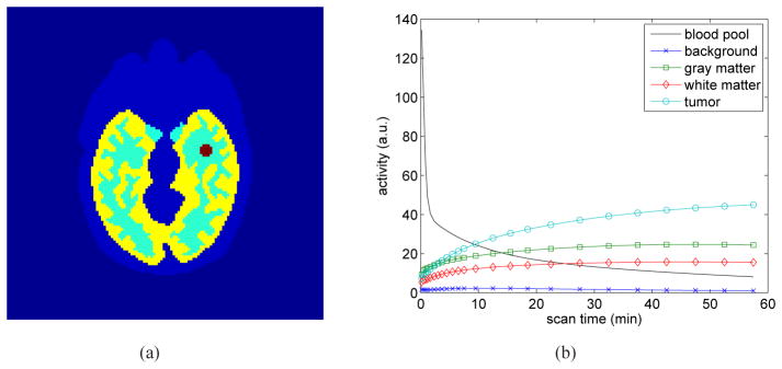
The simulation settings. (a) a Zubal brain phantom composed of gray matter, white matter and a small tumor; (b) regional time activity curves

TABLE II.

The kinetic parameters used in the FDG PET simulation. The unit of K₁-k₄ is min⁻¹.

	fv	K1	k2	k3	k4
Background	0.01	0.010	0.100	0.001	0.001
Gray matter	0.05	0.116	0.254	0.116	0.011
White matter	0.03	0.059	0.149	0.090	0.013
Tumor	0.04	0.088	0.055	0.096	0.001

Fifty independent and identically-distributed noisy datasets were generated and processed independently by the direct reconstruction method and indirect method to estimate the images of kinetic parameters. The regularization parameters in both reconstruction methods were the same and covered a wide range of values: 0, 1 ×10⁻⁴, 3 ×10⁻⁴, 1 ×10⁻³, 3 ×10⁻³, 1 × 10⁻². Both methods used 200 iterations in the reconstruction step to guarantee convergence. At each iteration of the direct algorithm, two iterations of the modified Levenberg-Marquardt algorithm were used. In the indirect method, dynamic images were first reconstructed frame-by-frame using the regular MAP-EM algorithm [24] for static image reconstruction, then followed by the usual Levenberg-Marquardt algorithm with 100 iterations to estimate the kinetic parameters pixel-by-pixel. The weighting factor in the kinetic fitting in the indirect method was chosen to be the squared frame duration divided by the count of the frame. The initial values of the kinetic parameters in both reconstructions were set to 0.01 for all pixels. The lower bounds were set to 10⁻⁵ and the upper bounds were 1.0 for all the kinetic parameters. The influx rate

$$K_i=\frac{K_1{k}_3}{k_2+k_3},$$

which is the major parameter of interest in FDG PET studies [30], was calculated from the estimated micro-parameters for evaluating the two methods.

A. Comparison between direct and indirect reconstructions

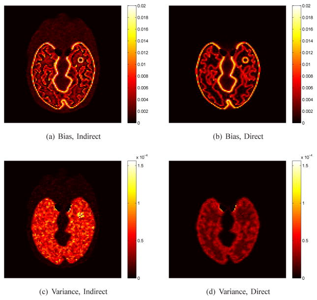
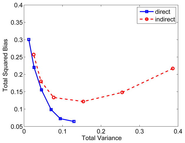
Fig. 2 shows the true and reconstructed K_i images by the direct method and indirect method. The regularization parameter used in this case was β = 3 ×10⁻⁴. In comparison, the result of the direct reconstruction is less noisy. The corresponding bias and variance images of the reconstructions are shown in Fig. 3. While the two methods have similar biases, the variance of the direct reconstruction is much lower than that of the indirect method. Fig. 4 plots the total squared bias against the total variance in the whole brain, by varying the regularization parameter β with β = 1 ×10⁻² corresponding to the leftmost point and β = 0 to the rightmost point. It shows that the direct reconstruction results in less variance at any given bias level than the indirect method.

Fig. 2.

True and reconstructed K_i parametric images using the indirect and direct algorithms (β = 0.0003).

Fig. 3.

The bias and variance images of K_i image reconstructed using the direct and indirect algorithms (β = 0.0003).

Fig. 4.

The total squared bias versus variance tradeoff of the influx rate K_i image reconstructed using the direct and indirect algorithms in the brain. Different points on the curves were obtained by varying the parameter β.

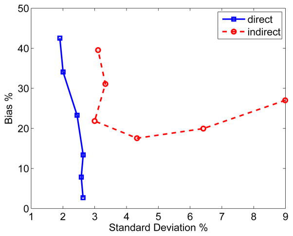
We also calculated the bias versus standard deviation tradeoff curve for region of interest (ROI) quantification, which takes into account of spatial correlation between image pixels. The ROI was chosen to be the tumor region. The trade-off curves are plotted in Fig. 5. Again, the standard deviation of the direct reconstruction is less than that of the indirect method at all bias levels.

Fig. 5.

The bias versus standard deviation tradeoff of tumor ROI quantification on K_i images reconstructed using the direct and indirect algorithms. Different points on the curves were obtained by varying the parameter β.

All of these results indicate that the direct reconstruction has a better quantification performance for K_i than the indirect reconstruction. While direct reconstruction using the Patlak model [31]–[33] can also generate K_i image for irreversible tracers, the Patlak model itself may introduce bias when applied to reversible tracers with k₄ > 0 (see [39] for example). In addition to the estimation of K_i, the proposed method can offer better parametric images of other kinetic parameters as well. As an example, Fig. 6 shows the reconstructed k₃ images by the direct approach and the indirect approach, both with the same regularization parameter β = 0.0003. Cleary the direct reconstruction result has much less noise than the indirect reconstruction result while maintaining the same spatial resolution.

Fig. 6.

The true and reconstructed k₃ images by the indirect and direct algorithms (β = 0.0003).

B. Comparison with previous optimization transfer algorithm

The convergence rate of the proposed algorithm (the optimization transfer with EM surrogate, OT-EM) was compared with one of our previous algorithms (optimization transfer with separable paraboloidal surrogate, OT-SP) [13]. We used two different measures to evaluate the convergence speed: normalized difference of the penalized log-likelihood and mean squared error (MSE) of reconstructed K_i images. The normalized likelihood difference at iteration n is calculated by

$$L_n=\frac{{\mathrm{\Phi }}^{\text{ref}}-{\mathrm{\Phi }}_n}{{\mathrm{\Phi }}^{\text{ref}}-{\mathrm{\Phi }}_1}$$ (40)

where Φ^ref is the reference value obtained at convergence. The advantage of using the normalized likelihood difference is that we can easily compare the convergence rate of different algorithms using a log-scale plot. The mean squared error of a reconstructed image at iteration n is calculated by

$$E_n=\frac{1}{n_j}\sum _{j=1}^{n_j}{(x_j^n-x_j^{\text{ref}})}^2$$ (41)

where xⁿ is the image reconstructed at iteration n, x^ref is the reference image obtained at convergence.

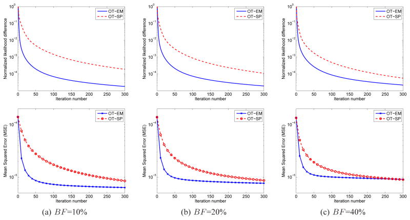
To investigate the effect of background (randoms and scatters) fraction BF on the convergence speed, we simulated three levels of background in the sinograms: BF = 10%, BF = 20% and BF = 40%. The OT-EM and OT-SP algorithms used the same regularization parameter β = 3 × 10⁻⁴ and started from the same uniform initials. The results of the OT-SP at iteration 5000 were used as the reference for calculating the normalized likelihood difference and mean squared error.

Fig. 7 shows the comparisons of the normalized likelihood difference and mean squared errors of the two direct algorithms as a function of iteration number. Both results show that the OT-EM algorithm is faster than the OT-SP algorithm. The speed-up of the OT-EM over the OT-SP becomes greater as the background fraction reduces, because the OT-SP algorithm uses a non-tight paraboloidal surrogate function and hence becomes slower when the fraction of background is low. When the background fraction is at 10%, the OT-SP requires more than 300 iterations to reach the same likelihood value and mean squared error as that achieved by the OT-EM with 50 iterations. The computational costs per iteration of the OT-SP and OT-EM are comparable. The former requires one more backprojection to compute the curvature of the paraboloidal surrogate, while the latter takes more computation time in the fitting step to calculate the logarithm. The real CPU times are about 9 seconds per iteration for the OT-EM and 10 seconds per iteration for the OT-SP, when implemented in MATLAB running on a 2.4 GHz CPU.

Fig. 7.

Comparisons of normalized likelihood (first row) and mean squared error (second row) of the penalized likelihood direct reconstructions using the optimization transfer approaches with the SP surrogate and with the EM surrogate for three different background fractions: (a) BF =10%, (b) BF =20% and (c) BF =40%.

C. Comparison with other algorithms

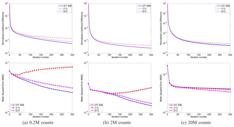
We compared the OT-EM algorithm with two direct reconstruction algorithms proposed by others [11], [21]. Both algorithms solve the image space maximum likelihood problem using a weighted least squares formulation. Uniform weight was used in [11] and nonuniform weight derived from an one-step-late approach was used in [21]. To our knowledge no proof of convergence has been established for either of the algorithm.

Fig. 8 compares the normalized likelihood difference and mean squared errors of the OT-EM algorithm and the algorithms by [11] and [21] for the Zubal data. Three different count levels (0.2M, 2M and 20M) were studied. The regularization parameter β in the OT-EM was set to 0 because the other two algorithms are only applicable to maximum likelihood reconstruction. The result of the algorithm in [21] at iteration 5000 was used as the reference. The plots show that the OT-EM is faster than the algorithm in [11] at all the count levels and can achieve faster convergence and lower MSE than the algorithm in [21] for lower-count data.

Fig. 8.

Comparison of the normalized likelihood difference (first row) and mean squared error (second row) of the maximum likelihood reconstruction using the OT-EM algorithm and the algorithms in [11] and [21] at three different count levels.

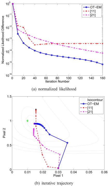
To demonstrate the potential non-monotonicity of the empirical algorithms, we also simulated a two-pixel toy example using a system matrix $\mathit{P}={\left[\begin{array}{ccc}0.5& 0.8& 0.2\\ 0.5& 0.2& 0.8\end{array}\right]}^T$ and two-tissue compartment model with the kinetic parameters [f_v, K₁, k₂, k₃, k₄]^T = [0.01, 0.1, 0.01, 0.01, 0.01]^T for pixel 1 and [f_v, K₁, k₂, k₃, k₄]^T = [0.01, 1.0, 1.0, 0.01, 0.01]^T for pixel 2. The input function and scanning schedule are the same as those used in the Zubal phantom simulation. One thousand events were simulated with a 20% background. Initial guess was 0.03 for all of the kinetic parameters. The lower bound for parameter estimate was set to 10⁻⁵ for all the parameters and the upper bound was 1.0 for f_v and 2.0 for K₁ to k₄.

Fig. 9(a) shows the normalized likelihood difference of the OT-EM and the algorithms in [11] and [21], using the result of the algorithm in [21] at iteration 5000 as the reference point. The trajectories of the estimated k₂ of the two pixels are plotted in figure 9(b) for the three algorithms, where the isocontours of the likelihood were drawn by varying k₂ parameter values while fixing other parameters at their reference values. The estimates by the algorithms in [11] and [21] at iteration 5000 are also marked in the figure. Both the OT-EM and the algorithm in [21] converged to the same optimum solution, but the OT-EM was much faster. The algorithm in [11] was non-monotonic and converged to a solution away from the optimum.

Fig. 9.

Comparison of (a) the likelihood and (b) the trajectory of estimated k₂ by different direct reconstruction algorithms in the two-pixel simulation. The noise-free ground truth is marked by ◇ in (b). All algorithms started from the same initialization.

V. Application to Real 4D Data

We have applied the OT-EM algorithm to a dynamic brain scan of a nonhuman primate. The data were acquired on a microPET P4 scanner (Siemens, Knoxville, TN). The radiotracer was ¹¹C-SCH 23390 which binds to dopamine D1 receptors in the brain [34]. The scan consists of 20 time frames over 45 minutes: 10×60 s, 5×120 s, 5×300 s. A transmission scan was used for estimating the attenuation map. Randoms were pre-corrected using the delayed window technique. The expected scatter sinograms were estimated by the single-scatter simulation method [35]. Images were reconstructed using an array of 128 × 128 × 63 voxels with a voxel size of 1.0 × 1.0 × 1.2 mm³.

The simplified reference tissue model (SRTM) was used for kinetic fitting of the ¹¹C-SCH 23390 data [36]. The cerebellum was chosen as the reference region. The tissue time activity curve is modeled by [37], [38]

$$C_{\text{T}}(t)={\theta }_1{C}_{\text{r}}(t)+{\theta }_2{C}_{\text{r}}(t)\otimes exp(-{\theta }_{3}t),$$ (42)

where θ₁ is the relative delivery rate from plasma to tissue, θ₂ and θ₃ can be interpreted as the transport rates of the target tissue relative to the reference region. C_r(t) is the reference TAC. The distribution volume ratio (DVR) of interest is calculated by

$$\text{DVR}={\theta }_1+{\theta }_2/{\theta }_3,$$ (43)

which is related to the binding potential (BP) via DVR = BP + 1.

We used both the indirect and direct methods to reconstruct the DVR parametric image. In the indirect method, the regular MAP-EM algorithm with 200 iterations was used to reconstruct dynamic emission images, then followed by the LM fitting with 100 iterations to obtain the weighted least squares estimates of the kinetic parameters θ₁, θ₂ and θ₃. The weighting factor in the fitting was set to the squared time duration divided by the total count of each frame [37]. The initial estimates in both methods were θ₁ = 1.0, θ₂ = 1.0, θ₃ = 0.1. The lower and upper bounds of (θ₁, θ₂, θ₃) were set to [10⁻⁵, 5.0], [10⁻⁵, 5.0] and [0.03, 0.6], respectively. In the direct method, the OT-EM algorithm was run for 200 iterations with two sub-iterations of the modified LM algorithm in the penalized likelihood fitting step.

Region-of-interest (ROI) quantification was performed on the DVR images estimated using the direct and indirect reconstruction methods. To define ROIs, the dynamic sinograms were summed up and reconstructed to form a single static image. One slice of the static reconstruction is shown in figure 10. Two ROIs were drawn in the striatal regions and four spheres of 8 mm in diameter were drawn in the brain background. Mean uptakes in the striatal regions and the average standard deviation in the background regions were computed for comparison.

Fig. 10.

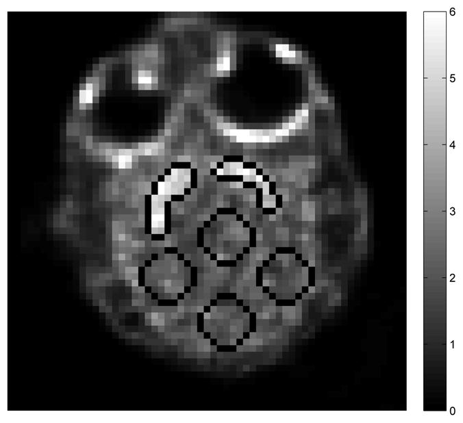
Striatal targets and background ROIs drawn on the reconstructed image of the sinogram summed over the whole dynamic scans.

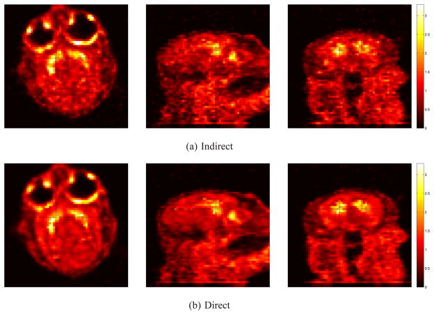
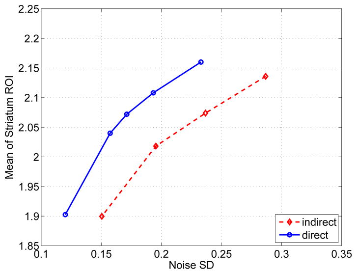
Figure 11 shows the DVR images reconstructed using the indirect and direct methods. Both methods used the same initial estimates of the kinetic parameters. The regularization parameter β for the indirect reconstruction was 100. The regularization parameter for the direct reconstruction was β = 200 in order to match the mean value of the striatal regions to that of the indirect reconstruction. Fig. 12 plots the mean uptake of the striatal ROIs versus background noise curve by varying the regularization parameter with β = 0 corresponding to the rightmost point and β = 1000 corresponding to the leftmost point. The second rightmost point on the indirect curve and the third rightmost point on the direct curve correspond to the images shown in figure 11, respectively. In comparison, the direct reconstruction reduces noise in the brain at any matched mean value of the striatum ROIs.

Fig. 11.

The estimated DVR images of the real primate brain data using (a) the indirect and (b) the direct methods. The three columns represent the transverse, sagittal and coronal slices of each 3D volume, respectively.

Fig. 12.

ROI mean of the striatum regions versus background standard deviation of the indirect and direct reconstructions. The curves are plotted by varying the regularization parameter β.

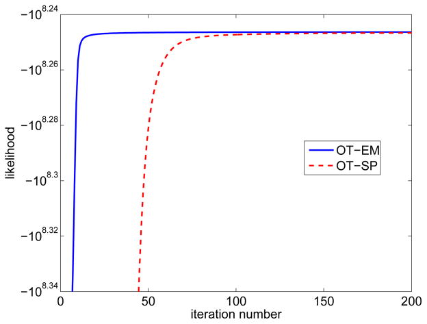
The brain data were also reconstructed using the OT-SP algorithm with β = 200. The penalized likelihood of the proposed OT-EM is compared with that of the OT-SP as shown in Fig. 13. Both algorithms started from the same initialization. The OT-EM is clearly faster than the OT-SP algorithm.

Fig. 13.

Comparison of convergence rate of the penalized likelihood direct reconstruction using the OT-SP and OT-EM algorithms for the real 4D primate data. Both approaches start from the same initialization.

VI. Conclusions

This paper presents a new optimization transfer approach for penalized likelihood direct reconstruction of nonlinear parametric images using the EM surrogate functions. Each iteration of the proposed algorithm consists of an EM-like dynamic image update, a spatial image smoothing, and a pixel-wise penalized likelihood kinetic fitting. The algorithm does not require a positive background in sinogram data and hence complements our previous generalized algorithm for direct reconstruction. Computer simulations validate that the direct reconstruction algorithm can have a better quantification performance than the indirect algorithm for estimation of parametric images. Application of the algorithm to a real brain scan also showed promising results.

References

- 1.Kordower JH, Emborg ME, Bloch J, et al. Neurodegeneration prevented by lentiviral vector delivery of GDNF in primate models of Parkinson’s disease. Science. 2000;290(5492):767–773. doi: 10.1126/science.290.5492.767. [DOI] [PubMed] [Google Scholar]
- 2.Gill SS, Patel NK, Hotton GR, et al. Direct brain infusion of glial cell line-derived neurotrophic factor in Parkinson disease. Nature Medicine. 2003;9(5):589–595. doi: 10.1038/nm850. [DOI] [PubMed] [Google Scholar]
- 3.Visser E, Philippens M, Kienhorst L, Kaanders J, Corstens F, de Geus-Oei L, Oyen W. Comparison of tumor volumes derived from glucose metabolic rate maps and SUV maps in dynamic 18F-FDG PET. Journal of Nuclear Medicine. 2008;49(6):892–898. doi: 10.2967/jnumed.107.049585. [DOI] [PubMed] [Google Scholar]
- 4.Tsoumpas C, Turkheimer FE, Thielemans K. A survey of approaches for direct parametric image reconstruction in emission tomography. Med Phys. 2008;35(9):3963–3971. doi: 10.1118/1.2966349. [DOI] [PubMed] [Google Scholar]
- 5.Rahmim A, Tang J, Zaidi H. Four-dimensional image reconstruction strategies in dynamic PET: Beyond conventional independent frame reconstruction. Med Phy. 2009;36(8):3654–3670. doi: 10.1118/1.3160108. [DOI] [PubMed] [Google Scholar]
- 6.Matthews J, Bailey D, Price P, Cunningham V. The direct calculation of parametric images from dynamic PET data using maximum-likelihood iterative reconstruction. Physics in Medicine and Biology. 1997;42(6):1155–1173. doi: 10.1088/0031-9155/42/6/012. [DOI] [PubMed] [Google Scholar]
- 7.Reutter BW, Gullberg GT, Huesman RH. Kinetic parameter estimation from attenuated SPECT projection measurements. IEEE Transactions on Nuclear Science. 1998;45(6):3007–3013. [Google Scholar]
- 8.Meikle SR, Matthews JC, Cunningham VJ, Bailey DL, Livieratos L, Jones T, Price P. Parametric image reconstruction using spectral analysis of PET projection data. Physics in Medicine and Biology. 1998;43(3):651–666. doi: 10.1088/0031-9155/43/3/016. [DOI] [PubMed] [Google Scholar]
- 9.Vanzi E, Formiconi AR, Bindi D, Cava GL, Pupi A. Kinetic parameter estimation from renal measurements with a three-headed SPECT system: A simulation study. IEEE Transactions on Medical Imaging. 2004;23(3):363–373. doi: 10.1109/TMI.2004.824149. [DOI] [PubMed] [Google Scholar]
- 10.Kamasak ME, Bouman CA, Morris ED, et al. Direct reconstruction of kinetic parameter images from dynamic PET data. IEEE Trans Med Im. 2005;24(5):636–650. doi: 10.1109/TMI.2005.845317. [DOI] [PubMed] [Google Scholar]
- 11.Reader A, Matthews J, Sureau F, et al. Iterative kinetic parameter estimation within fully 4D PET image reconstruction. IEEE Nucl Sci Syp & Med Im Conf. (3) 2006:1752–56. [Google Scholar]
- 12.Yan J, Wilson BP, Carson RE. Direct 4D list mode parametric reconstruction for PET with a novel EM algorithm. IEEE Nucl Sci Syp & Med Im Conf. 2008 doi: 10.1109/NSSMIC.2008.4774103. [DOI] [PMC free article] [PubMed] [Google Scholar]
- 13.Wang G, Qi J. Generalized algorithms for direct reconstruction of parametric images from dynamic PET data. IEEE Trans Med Im. 2010;28(11):1717–1726. doi: 10.1109/TMI.2009.2021851. [DOI] [PMC free article] [PubMed] [Google Scholar]
- 14.Lange K, Hunter DR, Yang I. Optimization transfer using surrogate objective functions. Journal of Computational and Graphical Statistics. 2000;9(1):1–20. [Google Scholar]
- 15.Fessler JA, Erdogan H. A paraboloidal surrogates algorithm for convergent penalized-likelihood emission image reconstruction. 1998 IEEE Nuclear Science Syposium and Medical Imaging Conference. 1998;2:1132–5. [Google Scholar]
- 16.Dempster AP, Laird NM, Rubin DB. Maximum likelihood from incomplete data via the EM algorithm. Journal of the Royal Statistical Society, Series B. 1977;39(1):1–38. [Google Scholar]
- 17.Wang G, Qi J. Acceleration of direct reconstruction of linear parametric images using nested algorithms. Phys Med Bio. 2010;55(5):1505–1517. doi: 10.1088/0031-9155/55/5/016. [DOI] [PMC free article] [PubMed] [Google Scholar]
- 18.Shepp LA, Vardi Y. Maximum likelihood reconstruction for emission tomography. IEEE Transactions on Medical Imaging. 1982;1(2):113–122. doi: 10.1109/TMI.1982.4307558. [DOI] [PubMed] [Google Scholar]
- 19.Lange K, Carson RE. EM reconstruction algorithms for emission and transmission tomography. Journal of Computer Assisted Tomography. 1984;8(2):306–316. [PubMed] [Google Scholar]
- 20.Wang G, Qi J. Direct reconstruction of nonlinear parametric images for dynamic PET using nested optimization transfer. IEEE Nuclear Science Symposium and Medical Imaging Conference. 2010 Nov; (abstract only) [Google Scholar]
- 21.Matthews JC, Angelis GI, Kotasidis FA, Markiewicz PJ, Reader AJ. Direct reconstruction of parametric images using any spatiotemporal 4D image based model and maximum likelihood expectation maximisation. IEEE Nuclear Science Symposium and Medical Imaging Conference. 2010 Nov;:2435–2441. [Google Scholar]
- 22.Schmidt KC, Turkheimer FE. Kinetic modeling in positron emission tomography. Quarterly Journal of Nuclear Medicine. 2002;46(1):70–85. [PubMed] [Google Scholar]
- 23.Carson RE, Lange K. The EM parametric image reconstruction algorithm. Journal of America Statistics Association. 1985;80(389):20–22. [Google Scholar]
- 24.De Pierro AR. A modified expectation maximization algorithm for penalized likelihood estimation in emission tomography. IEEE Transactions on Medical Imaging. 1995;14(1):132–137. doi: 10.1109/42.370409. [DOI] [PubMed] [Google Scholar]
- 25.Marquardt DW. An algorithm for least-squares estimation of nonlinear parameters. Journal of the Society for Industrial and Applied Mathematics. 1963;11(2):431–441. [Google Scholar]
- 26.Madsen K, Nielsen HB, Tingleff O. Methods for non-linear least squares problems. Tech rep, Technical University of Denmark. 2004 [Google Scholar]
- 27.Zubal IG, Harrell CR, Smith EQ, Rattner Z, Gindi G, Hoffer PB. Computerized three-dimensional segmented human anatomy. Medical Physics. 1994;21(2):299–302. doi: 10.1118/1.597290. [DOI] [PubMed] [Google Scholar]
- 28.Feng DG, Wong KP, Wu CM, Siu WC. A technique for extracting physiological parameters and the required input function simultaneously from PET image measurements: Theory and simulation study. IEEE Transactions on Information Technology in Biomedicine. 1997;1(4):243–254. doi: 10.1109/4233.681168. [DOI] [PubMed] [Google Scholar]
- 29.Spence AM, Muzi M, Graham MM, et al. Glucose metabolism in human malignant gliomas measured quantitatively with PET, 1-[C-11]glucose and FDG: analysis of the FDG lumped constant. Journal of Nuclear Medicine. 1998;39(3):440–448. [PubMed] [Google Scholar]
- 30.Huang SC, Phelps ME, Hoffman EJ, Kuhl DE. Error sensitivity of fluorodeoxyglucose method for measurement of cerebral metabolic-rate of glucose. Journal of Cerebral Blood Flow and Metabolism. 1981;1(4):391–401. doi: 10.1038/jcbfm.1981.43. [DOI] [PubMed] [Google Scholar]
- 31.Wang G, Qi J. Maximum a posteriori reconstruction of the Patlak parametric image from sinograms in dynamic PET. Physics in Medicine and Biology. 2008;53(3):593–604. doi: 10.1088/0031-9155/53/3/006. [DOI] [PubMed] [Google Scholar]
- 32.Tsoumpas C, Turkheimer FE, Thielemans K. Study of direct and indirect parametric estimation methods of linear models in dynamic positron emission tomography. Medical Physics. 2008;35(4):1299–1309. doi: 10.1118/1.2885369. [DOI] [PubMed] [Google Scholar]
- 33.Tang J, Kuwabara H, Wong DF, Rahmim A. Direct 4D reconstruction of parametric images incorporating anato-functional joint entropy. Physics in Medicine and Biology. 2010;55(15):4261–4272. doi: 10.1088/0031-9155/55/15/005. [DOI] [PMC free article] [PubMed] [Google Scholar]
- 34.Farde L, Halldin C, Sone-Elander S, Sedvall G. PET analysis of human dopamine receptor subtypes using 11C-SCH 23390 and 11C-raclopride. Psychopharmacology. 1987;92(3):278–284. doi: 10.1007/BF00210831. [DOI] [PubMed] [Google Scholar]
- 35.Watson CC. New, faster, image-based scatter correction for 3D PET. IEEE Transactions on Nuclear Science. 2000;47(4):1587–1594. [Google Scholar]
- 36.Lammertsma AA, Hume SP. Simplified reference tissue model for PET receptor studies. Neuroimage. 1996;4(3):153–158. doi: 10.1006/nimg.1996.0066. [DOI] [PubMed] [Google Scholar]
- 37.Gunn RN, Lammertsma AA, Hume SP, Cunningham VJ. Parametric imaging of ligand-receptor binding in PET using a simplified reference region model. Neuroimage. 1997;6(4):279–287. doi: 10.1006/nimg.1997.0303. [DOI] [PubMed] [Google Scholar]
- 38.Ichise M, Liow JS, Lu JQ, Takano A, Carson RE. Linearized reference tissue parametric imaging methods: application to [11C]DASB Positron Emission Tomography studies of the serotonin transporter in human brain. Journal of Cerebral Blood Flow and Metabolism. 2003;22(10):1271–1281. doi: 10.1097/01.WCB.0000085441.37552.CA. [DOI] [PubMed] [Google Scholar]
- 39.Yu AS, Lin HD, Huang SC, Phelps ME, Wu HM. Quantication of cerebral glucose metabolic rate in mice using 18F-FDG and small-animal PET. Journal of Nuclear Medicine. 2009;50(6):966–973. doi: 10.2967/jnumed.108.060533. [DOI] [PMC free article] [PubMed] [Google Scholar]