Body-Wide Hierarchical Fuzzy Modeling, Recognition, and Delineation of Anatomy in Medical Images

Abstract

To make Quantitative Radiology (QR) a reality in radiological practice, computerized body-wide automatic anatomy recognition (AAR) becomes essential. With the goal of building a general AAR system that is not tied to any specific organ system, body region, or image modality, this paper presents an AAR methodology for localizing and delineating all major organs in different body regions based on fuzzy modeling ideas and a tight integration of fuzzy models with an Iterative Relative Fuzzy Connectedness (IRFC) delineation algorithm. The methodology consists of five main steps: (a) gathering image data for both building models and testing the AAR algorithms from patient image sets existing in our health system; (b) formulating precise definitions of each body region and organ and delineating them following these definitions; (c) building hierarchical fuzzy anatomy models of organs for each body region; (d) recognizing and locating organs in given images by employing the hierarchical models; and (e) delineating the organs following the hierarchy. In Step (c), we explicitly encode object size and positional relationships into the hierarchy and subsequently exploit this information in object recognition in Step (d) and delineation in Step (e). Modality-independent and dependent aspects are carefully separated in model encoding. At the model building stage, a learning process is carried out for rehearsing an optimal threshold-based object recognition method. The recognition process in Step (d) starts from large, well-defined objects and proceeds down the hierarchy in a global to local manner. A fuzzy model-based version of the IRFC algorithm is created by naturally integrating the fuzzy model constraints into the delineation algorithm.

The AAR system is tested on three body regions – thorax (on CT), abdomen (on CT and MRI), and neck (on MRI and CT) – involving a total of over 35 organs and 130 data sets (the total used for model building and testing). The training and testing data sets are divided into equal size in all cases except for the neck. Overall the AAR method achieves a mean accuracy of about 2 voxels in localizing non-sparse blob-like objects and most sparse tubular objects. The delineation accuracy in terms of mean false positive and negative volume fractions is 2% and 8%, respectively, for non-sparse objects, and 5% and 15%, respectively, for sparse objects. The two object groups achieve mean boundary distance relative to ground truth of 0.9 and 1.5 voxels, respectively. Some sparse objects – venous system (in the thorax on CT), inferior vena cava (in the abdomen on CT), and mandible and naso-pharynx (in neck on MRI, but not on CT) – pose challenges at all levels, leading to poor recognition and/or delineation results. The AAR method fares quite favorably when compared with methods from the recent literature for liver, kidneys, and spleen on CT images. We conclude that separation of modality-independent from dependent aspects, organization of objects in a hierarchy, encoding of object relationship information explicitly into the hierarchy, optimal threshold-based recognition learning, and fuzzy model-based IRFC are effective concepts which allowed us to demonstrate the feasibility of a general AAR system that works in different body regions on a variety of organs and on different modalities.

1. INTRODUCTION

1.1 Background

Since the birth of radiology in 1895, the emphasis in clinical radiology has been on human visualization of internal structures. Although various tomographic image modalities evolved subsequently for deriving anatomic, functional, and molecular information about internal structures, the emphasis on human visualization continued and the practice of clinical radiology has remained mostly descriptive and subjective. Quantification is amply employed in radiology in clinical research. However, in clinical radiological practice, this is not common. In the qualitative mode, quantifiable and/or subtle image information is underutilized, interpretations remain subjective, and subtle changes at early disease stages or due to therapeutic intervention may be underestimated or missed (Torigian et al. 2007). It is generally believed now that if Quantitative Radiology (QR) can be brought to routine clinical practice, numerous advances can be made including: improved sensitivity, specificity, accuracy, and precision of early disease diagnosis; more objective and standardized response assessment of disease to treatment; improved understanding of what is “normal”; increased ease of disease measurement and reporting; and discovery of new disease biomarkers.

To make QR a reality, we believe that computerized Automatic Anatomy Recognition (AAR) during radiological image interpretation becomes essential. To facilitate AAR, and hence eventually QR, and focusing only on the anatomic aspects of shape, geography, and architecture of organs, while keeping the larger goal in mind, we present in this paper a novel fuzzy strategy for building body-wide anatomic models, and for utilizing these models for automatically recognizing and delineating body-wide anatomy in given patient images.

1.2 Related work

Image segmentation – the process of recognizing and delineating objects in images – has a rich literature spanning over five decades. From the perspective of the direction in which this field is headed, it is useful to classify the methods developed to date into three groups: (a) Purely image-based, or pI approaches (Beucher 1992, Boykov et al. 2001, Kass et al. 1987, Malladi et al. 1995, Mumford and Shah 1989, Udupa and Samarasekera 1996), wherein segmentation decisions are made based entirely on information derived from the given image; (b) Object model-based, or OM approaches (Ashburner and Friston 2009, Cootes et al. 2001, Heimann and Meinzer 2009, Pizer et al. 2003, Shattuck et al. 2008, Staib and Duncan 1992,), wherein known object shape and image appearance information over a population are first codified in a model and then utilized on a given image to bring constraints into the segmentation process; (c) Hybrid approaches (Chen and Bagci 2011, Hansegrad et al. 2007, Horsfield et al. 2007, Liu and Udupa 2009, Rousson and Paragios 2008, Shen et al. 2011, van der Lijn et al. 2012, Zhou and Bai 2007), wherein the delineation strengths of the pI methods are combined synergistically with the global object recognition capabilities of the OM strategies. pI algorithms predate other approaches, and they still continue to seek new frontiers. OM approaches go by various names such as statistical models and probabilistic atlases, and continue to be pursued aggressively. Particularly, atlas-based techniques have gained popularity in brain MR image segmentation and analysis (Cabezas et al. 2011). Hybrid approaches hold much promise for AAR and QR and are currently very actively investigated. Since our focus in this paper is the body torso, and since the nature of the images and of the objects and challenges encountered are different for these regions (from, for example, for the brain), our review below will focus mainly on methods developed for the torso.

Since the simultaneous consideration of multiple objects offers better constraints, in recent years, multi-object strategies have been studied under all three groups of approaches to improve segmentation. Under pI approaches, the strategy sets up a competition among objects for delineating their regions/boundaries (e.g.; Bogovic et al. 2013, Saha and Udupa 2001). In OM approaches, the strategy allows including inter-relationships among objects in the model to influence their localization and delineation (e.g.; Cerrolaza et al. 2012, Duta and Sonka 1998). In hybrid approaches, multi-object strategies try to strengthen segmentability by incorporating relevant information in model building, object recognition/localization, and subsequently also in delineation via the pI counterpart of the synergistic approach (Chen et al. 2012, Chu et al. 2013, Linguraru et al. 2012, Lu et al. 2012, Meyer et al. 2011, Okada et al. 2008, Shen et al. 2011, Tsechpenakis and Chatzis 2011). Motivated by applications (such as semantic navigation) where the focus is just locating objects in image volumes and not delineating them, a separate group of methods has been emerging (Criminisi et al. 2013, Zhou et al. 2005, Zhou et al. 2013). They use features characterizing the presence of whole organs or specific anatomic aspects of organs (such as the femoral neck and head) combined with machine learning techniques to locate objects in image volumes by finding the size, location, and orientation of rectangular bounding boxes that just enclose the anatomic entities.

The state-of-the-art in image segmentation seems to leave several gaps that hinder the development of a body-wide AAR system. First, while multi-object strategies have clearly shown superior performance for all approaches, in all published works they have been confined to only a few (three to five) selected objects and have not taken into account an entire body region or all of its major organs, the only exception being (Baiker et al. 2010), whose focus was whole body segmentation of mice on micro CT images. Second, and as a result, there is no demonstrated single method that operates on different body regions, on all major organs in each body region, and at different modalities. Third, all reported modeling strategies have a statistical framework, either as statistical models of shape and intensity pattern of appearance of objects in the image or as atlases, and none taking a fuzzy approach, except (Zhou and Rajapakse 2005) and our previous work (Miranda et al. 2008, Miranda et al. 2009), both in the brain only. Fuzzy set concepts have been used extensively otherwise in image processing and 3D visualization. Fuzzy modeling approaches allow bringing anatomic information in an all-digital form into graph theoretic frameworks designed for object recognition and delineation, obviating the need for (continuous) assumptions made otherwise in statistical approaches about shapes, random variables, their independence, functional form of density distributions, etc. They also allow capturing information about uncertainties at the patient level (e.g., blur, partial volume effects) and population level, and codification of this information within the model. Fourth, objects have complex inter-relationships in terms of their geographic layout. Learning this information over a population and encoding this explicitly in an object hierarchy can facilitate object localization considerably. Although several multi-object methods have accounted for this relationship indirectly, its direct incorporation into modeling, object recognition, and delineation in an anatomic hierarchical order has not been attempted. The AAR approach presented in this paper is designed to help overcome these gaps.

1.3 Outline of paper and approach

We start off by describing a novel hierarchical fuzzy modeling framework for codifying prior population information about object assemblies in Section 2. In Section 3, we delineate methods for automatically recognizing objects in given patient images that employ these hierarchical models. We present fuzzy-connectedness-based object delineation techniques in Section 4 that employ the modified fuzzy models found at recognition as constraints in delineation. We demonstrate and evaluate the applicability of the AAR methodology in Section 5 on three different body regions – thorax, abdomen, and neck - on different modalities. A comparison to methods from recent literature, the lessons learned, our conclusions, and the challenges we encountered are examined in Section 6. The AAR approach has five unique characteristics: (1) direct hierarchical codification of the prior object geographic and geometric relationship information; (2) a “what-you-see-is-what-you-get” entirely digital fuzzy modeling strategy; (3) hierarchical object recognition strategies that go from a broader gestalt to narrower specifics in locating objects; (4) demonstrated generality of applicability of the same approach to different organ systems, body regions, and modalities; and (5) adaptability of the system to different applications.

The AAR approach is graphically summarized in Figure 1. The body is divided into body regions B₁, …, B_K. Models are built for each specific body region ∈ {B₁, …, B_K} and each population group G (whatever way G is defined). Throughout this paper, and G are treated as variables, and each body region is considered separately and independent of other body regions. In Section 6, we will discuss briefly the issue of linking body regions for considering the whole body for the AAR schema. The three main blocks in Figure 1 correspond to model building, object recognition, and object delineation. A fuzzy model FM(O_l) is built separately for each of the L objects O_l in , and these models are integrated into a hierarchy chosen for . The output of the first step is a fuzzy anatomic model FAM( , G) of the body region for group G. This model is utilized in recognizing objects in a given patient image I of belonging to G in the second step. The hierarchical order is followed in this process. The output of this step is the set of transformed fuzzy models FM^T(O_l) corresponding to the state when the objects are recognized in I. These modified models and the image I form the input to the third step of object delineation which also follows the hierarchical order. The final output is in the form of delineated objects O₁^D, …, O_L^D, where each O_l^D is a binary image.

Figure 1.

A schematic representation of the AAR schema. The three main steps of model building, object recognition, and object delineation are explained in Sections 2, 3, and 4.

Very preliminary versions of some of the contents of this paper appeared in SPIE Medical Imaging conference proceedings in 2011, 2012, and 2013. Those papers did not contain the full details presented here on model building. More importantly, based on earlier experience many improvements are reported in this paper, none of which appeared earlier. Further, the recognition and delineation methods presented here have many novel elements. As a result, the entire AAR approach has changed substantially. Additional differences include comprehensive evaluation and the demonstration of the AAR scheme on multiple body regions.

2. BUILDING FUZZY MODEL OF BODY REGION

Notation

We will use the following notation throughout this paper. G: the population group under consideration. : the body region of focus. O₁, …, O_L : L objects or organs of (such as esophagus, pericardium, etc. for = Thorax). I = {I₁, …, I_N}: the set of images of for G from N subjects which are used for model building and for training the parameters of the AAR algorithms. I_n,l: the binary image representing the true delineation of object O_l in the image I_n ∈ I. I^b = {I_n,l : 1 ≤ n ≤ N & 1 ≤ l ≤ L} is the set of all binary images used for model building. FM(O_l): Fuzzy model of object O_l derived from the set of all binary images I^b_l = {I_n,l : 1 ≤ n ≤ N} of O_l. FAM( ,G): Fuzzy anatomy model of the whole object assembly in with its hierarchy. FM^T(O_l): Transformed (adjusted) FM(O_l) corresponding to the state when O_l is recognized in a given patient image I. O_l^D: Delineation of O_l in I represented as a binary image. Any image I will be represented by a pair I = (C, f), where C denotes a 3D rectangular array of voxels, and f is a mapping f: C → I where I is a set of integers¹ denoting the image intensities. For any binary image J = (C, f_b), we will use PAS(J) to denote the principal axes system derived from the set X of voxels of J with value 1. PAS(J) is described by the geometric center of X and the eigenvectors derived from X via principal component analysis.

Our description in the rest of Section 2 will follow the schematic of Figure 1. Table 1 in Appendix lists brief anatomic definitions of all objects from all three body regions considered in this paper.

2.1 Gathering image database for and G

This retrospective study was conducted following approval from the Institutional Review Board at the Hospital of the University of Pennsylvania along with a Health Insurance Portability and Accountability Act (HIPAA). The basic premise of our AAR approach is that the fuzzy anatomic model of for G should reflect near normal anatomy. Consequently, the cleanest way of gathering image data for model building will be to prospectively acquire image data in a well-defined manner from subjects in group G who are certified to be near normal. Such an approach would be expensive and may involve radiation exposure (in case of CT imaging). For developing the concepts and testing the feasibility of AAR, therefore, we have taken a vastly less expensive and simpler approach of utilizing existing human subject image data sets. For the thoracic and abdominal body regions, a board certified radiologist (co-author DAT) selected all image data sets (CT) from our health system patient image database in such a manner that the images appeared radiologically normal for the body region considered, with exception of minimal incidental focal abnormalities such as cysts, small pulmonary nodules, etc. Images with severe motion/streak artifacts or other limitations were excluded from consideration. For these two body regions, the population groups considered have an age range of approximately 50–60 years. This age range was selected to maximize our chances of finding sufficient number of near normal images. For the neck body region, we have utilized image data (MRI) previously acquired from normal subjects for the study of pediatric upper airway disorders. G in this instance is female subjects in the age range of 7–18. Our modeling schema is such that the population variables can be defined at any desired “resolution” in the future and the model can then be updated when more data are added.

Some organs in are better defined in a slice plane different from the slice plane used for imaging others. For example, for = neck, the best plane for slice imaging is sagittal for tongue and soft palate, while for the upper airways and other surrounding organs, axial slices are preferred. Our AAR methodology automatically handles organs defined in images with different orientations of digitization by representing image and object data in a fixed and common scanner coordinate system of reference.

2.2 Delineating objects of in the images in the database

There are two aspects to this task – forming an operational definition of both and the organs in in terms of their precise anatomic extent, and then delineating the objects following the definition. These considerations are important for building consistent and reliable models, and, in the future, if similar efforts and results for body-wide models are to be combined, exchanged, and standardized.

Definition of body regions and objects

Each body region is defined consistently in terms of a starting and ending anatomic location. For axial slice data, these locations are determined in terms of transverse slice positions. For example, for = Thorax, the body region is considered to extend axially from 5 mm below the base of the lungs to 15 mm above the apex of the lungs. Arms are not included in this study. For other orientations of slice planes in slice imaging, the same definitions are applied but translated into other planes. Similarly, each object included in is defined precisely irrespective of whether it is open-ended - because it straddles body regions (for example, esophagus) - or closed and contained within but is contiguous with other objects (for example, liver with hepatic portal vein, common hepatic artery, and bile duct). For each body region, we have created a document that delineates its precise definition and the specification of the components and boundaries of its objects. This document is used as a reference by all involved in generating data sets for model building. These definitions are summarized in the table included in Appendix.

Each body region is carved out manually, following its definition, from the data sets gathered for it. In our notation, I denotes the resulting set of such standard images that precisely cover as per definition. We assume the scanner coordinate system, SCS, as a common reference system with respect to which all coordinates will be expressed.

Delineation of objects

The objects of are delineated in the images of I, adhering to their definition, by a combination of methods including live wire, iterative live wire (Souza and Udupa 2006), thresholding, and manual painting, tracing and correction. To minimize human labor and to maximize precision and accuracy, algorithms in terms of a proper combination of these methods and the order in which objects are delineated are devised first, all of which operate under human supervision and interaction. For illustration, in the abdomen, to delineate subcutaneous adipose tissues (SAT) as an object, the skin outer boundary ASkn (as an object) is first segmented by using the iterative live wire method. Iterative live wire is a version of live wire in which once the object is segmented in one slice, the user commands next slice, the live wire then operates automatically in the next slice, and the process is continued until automatic tracing fails when the user resorts to interactive live wire again, and so on. Subsequently, the interface between the subcutaneous and visceral adipose compartments is delineated by using also the iterative live wire method. Once these two object boundaries are delineated, the subcutaneous and visceral components are delineated automatically by using thresholding and morphological operations. On MR images, the same approach works if background non-uniformity correction and intensity standardization (Nyul and Udupa 1999) are applied first to the images in I. If direct delineation by manual tracing or even by using live wire is employed, the process would become complicated (because of the complex shape of the adipose and visceral compartments) and much more labor intensive.

Because of the enormity of this task, a number of trainees, some with medical and biomedical but some with engineering background, were involved in accomplishing this task. All tracings were examined for accuracy by several checks – 3D surface renditions of objects from each subject in various object combinations as well as a slice-by-slice verification of the delineations overlaid on the gray images for all images. The set of binary images generated in this step for all objects is denoted by I^b = {I_n,l : 1 ≤ n ≤ N & 1 ≤ l ≤ L}. The set of binary images generated just for object O_l is denoted by I^b_l = {I_n,l : 1 ≤ n ≤ N}.

2.3 Constructing fuzzy object models

The Fuzzy Anatomy Model FAM( , G) of any body region for group G is defined to be a quintuple:

$$\mathit{FAM}(\mathcal{B},G)=(H,M,\rho ,\lambda ,\eta ).$$ (1)

Briefly, the meaning of the five elements of FAM( , G) is as follows. H is a hierarchy, represented as a tree, of the objects in ; see Figure 2. M is a collection of fuzzy models, one model per object in . ρ describes the parent-to-offspring relationship in H over G. λ is a set of scale factor ranges indicating the size variation of each object O_l over G. η represents a set of measurements pertaining to the objects in . A detailed description of these elements and the manner in which FAM( , G) is derived from I and I^b are presented below.

Figure 2.

(a) Hierarchy for whole body WB. (b) Hierarchy for Thorax. TSkn: Outer boundary of thoracic skin as an object; RS: Respiratory System; TSk: Thoracic Skeleton; IMS: Internal Mediastinum; RPS, LPS: Right & Left Pleural Spaces; TB: Trachea & Bronchi; E: Esophagus; PC: Pericardium; AS, VS: Arterial & Venous Systems. (c) Hierarchy for Abdomen. ASkn: Outer boundary of abdominal skin; ASk: Abdominal Skeleton; Lvr: Liver; ASTs: Abdominal Soft Tissues; SAT & VAT: Subcutaneous and Visceral Adipose Tissues; Kd: Kidneys; Spl: Spleen; Msl: Muscle; AIA: Aorta and Iliac arteries; IVC: Inferior Vena Cava; RKd & LKd: Right and Left Kidneys. (d) Hierarchy for Neck. NSkn: Outer boundary of skin in neck; A&B: Air & Bone; FP: Fat Pad; NSTs: Soft Tissues in neck; Mnd: Mandible; Phrx: Pharynx; Tnsl: Tonsils; Tng: Tongue; SP: Soft Palate; Ad: Adenoid; NP & OP: Nasopharynx and Oropharynx; RT & LT: Right and Left Tonsils.

Hierarchy H

This element describes the way the objects of are considered ordered anatomically as a tree structure. This order currently specifies the inclusion of an offspring object O_k anatomically in the parent object O_l.² While each has its own hierarchy, itself forms the offspring of a root denoting the whole body, WB, as shown in Figure 2. The hierarchies devised for the three body regions studied are shown in Figure 2. An object that is exactly a union of its offspring will be referred to as a composite object. Examples: RS, Fat, Kd, etc. Note that none of the skin objects is a composite object since the full body region inside the skin is not fully accounted for by the union of the offspring objects. The notion of composite objects is useful in combining objects of similar characteristics at a higher level of the hierarchy, which may make object recognition (and delineation) more effective. Thin tubular objects will be called sparse objects: TB, E, AS, VS, AIA, IVC, Phrx, NP, and OP. Compact, blob-like objects will be referred to as non-sparse: TSkn, RS, IMS, LPS, RPS, PC, ASkn, Fat, SAT, VAT, Lvr, Spl, Kd, RKd, LKd, NSkn, FP, NSTs, Tnsl, Tng, SP, Ad, RT, and LT. Some objects are a hybrid between these two types, consisting of both features. Examples: TSk, Ask, ASTs, A&B, and Mnd.

Fuzzy model set M

The second element M in the description of FAM( , G) represents a set of fuzzy models, M = {FM(O_l): 1 ≤ l ≤ L}, where FM(O_l) is expressed as a fuzzy subset of a reference set Ω_l ⊂ Z³ defined in the SCS; that is, FM(O_l) = (Ω_l, μ_l). The membership function μ_l(v) defines the degree of membership of voxel v ∈ Ω_l in the model of object O_l. Ideally, for any l, 1 ≤ l ≤ L, we would like the different samples of O_l in different subjects to differ by a transformation A_n,l involving translation, rotation, and isotropic scaling. Our idea behind the concept of the fuzzy model of an object is to codify the spatial variations in form from this ideal that may exist among the N samples of the object as a spatial fuzzy set, while also retaining the spatial relationship among objects in the hierarchical order.

Given the training set of binary images I^b_l of object O_l, we determine A_n,l, μ_l, and FM(O_l) for O_l as follows. We permit only such alignment operations, mimicking A_n,l, among the members of I^b_l, that are executed precisely without involving search and that avoid the uncertainties of local optima associated with optimization-based full-fledged registration schemas. In this spirit, we handle the translation, rotation, and scaling components of A_n,l in the following manner.

For translation and rotation, for each manifestation I_n,l of O_l in I^b_l, we determine, within SCS, the principal axes system PAS(I_n,l) of O_l. Subsequently, all samples are aligned to the mean center and principal axes³. The scale factor estimation is based on a linear size estimate (in mms) of each sample of O_l and resizing all samples to the mean size. The size of O_l in I_n,l is determined from $\sqrt{(e_1+e_2+e_3)}$, where e₁, e₂, and e₃ are the eigenvalues corresponding to the principal components of O_l in I_n,l.⁴

After aligning the members of I^b_l via A_n,l, a distance transform is applied to each transformed member for performing shape-based interpolation (Raya and Udupa 1990, Maurer et al. 2003), the distances are averaged over all members, and converted through a sigmoid function to obtain the membership values μ_l and subsequently FM(O_l).

Parent-to-offspring relationship ρ

This element describes the parent-to-offspring spatial relationship in H for all objects in . Since each object O_k has a unique parent, this relationship is represented by ρ = {ρ_k : 1 ≤ k ≤ L}⁵. For each O_k, ρ_k codifies the mean position as well as the orientation relationship between O_k and its parent over N samples. We adopt the convention that ρ₁ denotes the relationship of the root object of relative to SCS. Let GC_n,l be the geometric center of O_l in I_n,l. Then, the mean positional relationship P_l,k between O_l and O_k is considered to be the mean of the vectors in the set {GC_n,k − GC_n,l : 1≤ n ≤ N}. To find the mean orientation Q_l,k, we make use of the eigenvectors E¹_n,l, E²_n,l, and E³_n,l of the shape of O_l in I_n,l estimated over all N samples. We take an average of each Eⁱ_n,l over N samples for i = 1, 2, 3. However, for some n and i, Eⁱ_n,l may be more than 90 degrees from the average, in which case we replace Eⁱ_n,l by −Eⁱ_n,l while simultaneously replacing E^j_n,l by −E^j_n,l for some j different from i so as to keep the system right-handed. We then recalculate the average, and repeat until the eigenvector is within 90 degrees of the average. Then, starting from either the first or the third eigenvector, whichever has the eigenvalue farther from the second, we normalize and make the others orthogonal to it. Q_l,k is then taken to be the transformation that aligns the eigenvector system of the parent O_l with that mean orientation. This method guarantees a robust orientation estimate despite the 180-degrees switching property of eigenvectors.

In order not to corrupt ρ_k by the differences in size among subjects, before estimating ρ_k, the parent O_l and all offspring objects O_k of O_l are scaled with respect to the center GC_n,l of O_l as per a common scale factor, estimated for O_l via the method described above. The reasoning behind this scaling strategy is that an object and its entire offspring should be scaled similarly to retain their positional relationship information correctly.

Scale range λ

The fourth element λ of FAM( , G) is a set of scale factor ranges, λ = {λ_l = [λ^b_l, λ^h_l] : 1 ≤ l ≤ L}, indicating the size variation of each object O_l over its family I^b_l. This information is used in recognizing O_l in a given image to limit the search space for its pose; see Section 3.

Measurements η

This element represents a set of measurements pertaining to the object assembly in . Its purpose is to provide a database of normative measurements for future use. We are not exploring this aspect in this paper. However, this element also serves to improve our knowledge about object relationships (in form, geographical layout etc. in ) and thence in constructing better hierarchies for improving AAR. We will discuss this briefly in Section 5.

There are several parameters related to object recognition (Section 3) and delineation (Section 4), some of which are image modality specific. (They are identified by T₁^m and Th_l in Section 3 and σ_ψO, m_ϕO, m_ϕB, σ_ϕO, and σ_ϕB, in Section 4.) The values of these parameters are also considered part of the description of η. The definition of these parameters and the process of their estimation are described at relevant places in Sections 3 and 4 for ease of reading, although their actual estimation is done at the model building stage.

The fuzzy anatomy model FAM( , G) output by the model building process is used in performing AAR on any image I of for group G as described in Sections 3 and 4.

3. RECOGNIZING OBJECTS

We think of the process of what is usually referred to as “segmenting an object in an image” as consisting of two related phenomena – object recognition (or localization) and object delineation. Recognition is a high-level process of determining the whereabouts of the object in the image. Given this information for the object, its delineation is the meticulous low-level act of precisely indicating the space occupied by the object in the image. The design of the entire AAR methodology is influenced by this conceptual division. We believe that without achieving acceptably accurate recognition it is impossible to obtain good delineation accuracy. The hierarchical concept of organizing the objects for AAR evolved from an understanding of the difficulty involved in automatic object recognition. Once good recognition accuracy is achieved, several avenues for locally confined accurate delineation become available, as we discuss in Section 4. The goal of recognition in AAR is to output the pose (translation, rotation, and scaling) of FM(O_l), or equivalently the pose-adjusted fuzzy model FM^T(O_l), for each O_l in a given test image I of such that FM^T(O_l) matches the information about O_l present in I optimally.

The recognition process proceeds hierarchically as outlined in the procedure AAR-R presented below. In Step R₁, the root object is recognized first by calling algorithm R-ROOT⁶. Then, proceeding down the tree represented by H in the breadth-first order, other objects are recognized by calling algorithm R-OBJECT. The latter makes essential use of the parent fuzzy model and the parent-to-offspring relationship ρ encoded in FAM( , G).

Procedure AAR-R
Input:	An image I of , FAM( , G).
Output:	FMT(Ol), l = 1, …, L.
Begin
R1.	Call R-ROOT to recognize the root object in H;
R2.	Repeat
R3.	Find the next offspring Ok to recognize in H (see text);
R4.	Knowing FMT(Ol), ρk, and λk, call R-OBJECT to recognize Ok;
R5.	Until all objects are covered in H;
R6.	Output FMT(Ol), l = 1, …, L;
End

Two strategies are described here for each of algorithms R-ROOT and R-OBJECT. The first, a global approach, does not involve searching for the best pose. We call this the One-Shot Method since the model pose is determined directly by combining the prior information stored in FAM( , G) and information quickly gathered from the given image I. The one-shot method is used as initialization for a more refined second method called Thresholded Optimal Search.

One-Shot Method

A threshold interval Th₁ corresponding to the root object O₁ is applied to I followed by a morphological opening operation to roughly segment O₁ to produce a binary image J. The purpose of the morphological operation is to exclude as much as possible any significant extraneous material, such as the scanner table and patient clothing, from J. Then the transformed model FM^T(O₁) is found by applying a transformation T₁^m to FM(O₁). T₁^m is devised to express the mean relationship between the roughly segmented O₁ and the true segmentation of O₁ represented in the binary images I_n,1 ∈ I^b. The estimation of T₁^m is done at the model building stage of AAR as mentioned in Section 2.3. To determine T₁^m, similar thresholding and morphological operations are performed on each gray image I_n in the training set to obtain a rough segmentation of O₁, denoted J_n,1, in I_n. The relationship between this rough segmentation J_n,1 and the true segmentation I_n,1 of O₁ in I^b is found as a transformation T_n,1 that maps PAS(J_n,1) to PAS(I_n,1). The mean, denoted T₁^m, of such transformations over all training images is then found.

Once the root object O₁ is recognized, the poses for other objects in I in the hierarchy H are determined by combining (in the sense of composition) T₁^m with the parent to offspring relationship information stored in ρ_k for each parent-offspring pair. The transformed models FM^T(O_l) are then found from this information.

Thresholded Optimal Search

This is a strategy to refine the results obtained from the one-shot method. Its premise is that the overall image intensity of the objects in can be characterized by threshold intervals⁷ such that, at the model’s pose corresponding to the best match of the model with an underlying object in the given test image I, the mismatch between the thresholded result and the model is minimal. For MR images for this approach to make sense, it is essential to correct for background intensity nonuniformities first followed by intensity standardization (Nyul and Udupa 1999).

Suppose that at the model building stage, the optimal threshold interval Th_l for each object O_l has already been determined automatically from the training image set. We will explain below how this is accomplished. Then, at the recognition stage, the threshold for O_l is fixed at this learned value Th_l. Starting from the initial pose found by the one-shot method, a search is made within the pose space for an optimal pose p^* of the fuzzy model over I that yields the smallest sum of the volume of false positive and false negative regions, where the model itself is taken as the reference for defining false positive and negative regions. Specifically, let FM ^p(O_l)denote the fuzzy model of O_l at any pose p, expressed as an image, and let J denote the binary image resulting from thresholding I at Th_l. Then⁸,

$${\mathit{p}}^{\ast }\in \underset{\mathit{p}}{argmin}(\left|{FM}^p(O_l)-J\right|+\left|J-{FM}^p(O_l)\right|).$$ (2)

Image subtraction here is done in the sense of fuzzy logic, and |x| denotes the fuzzy cardinality of x, meaning that it represents the sum total of the membership values in x. The search space to find p^* is limited to a region around the initial pose. This region is determined from knowledge of ρ_k and its variation and the scale factor range λ_k. For the positional vector, we search in an ellipsoid with its axes in the coordinate axis directions and with length four times the standard deviation of the corresponding coordinate. When searching in orientation space, we search in an ellipsoid with its axes in the direction of the eigenvectors of the rotation vector distribution (covariance matrix) and with length four times the square root of the corresponding eigenvalue. (A rotation vector has magnitude equal to the angle of rotation and direction along the axis of right-handed rotation. The rotation referred to is the rotation of Q_l,k required to bring it into coincidence with Eⁱ_n,l.) For the scale factor, we search in an interval of size four times the standard deviation of the scale factor.

Determining Th_l at the model building stage

To estimate Th_l, we run a rehearsal of the recognition method described above as follows, essentially for attempting to learn the recognition process. Imagine we already built M and estimated ρ and λ. Suppose that we now run the recognition process on the training images. Since we do not know the optimal threshold but have the true segmentations, the idea behind this learning of the recognition process is to test recognition efficacy for each of a number of threshold intervals t and then select the interval Th_l that yields the best match of the model with the known true segmentations for each O_l. That is, if J_n(t) is the binary image resulting from thresholding the training image I_n at t, then

$${Th}_I\in \underset{\mathit{p},t}{argmin}\sum _n|(J_n(t)\times {FM}^{\mathit{p}}(O_l))-I_{n,I}|+|I_{n,I}-(J_n(t)\times {FM}^{\mathit{p}}(O_l))|.$$ (3)

Here, × denotes fuzzy intersection. In words, the optimal threshold Th_l is found by searching over the pose space over all training data sets and all thresholds the best match between the true segmentation of O_l with the result of thresholding I_n restricted to the model. In our implementation, 81 different values of the intervals are searched (9 for each end of the interval). The 9 positions for the lower end are the 5^th, 10^th, …, 45^th percentile values of the cumulative object intensity histogram determined from the training image set. Similarly, for the upper end, the positions are 55^th to 95^th percentile values.

To summarize, the thresholded optimal search method starts the search process from the initial pose found by the one-shot method. It uses the optimal threshold values Th_l determined at the training stage for each object O_l and finds the best pose for the fuzzy model of O_l in the given image I by optimally matching the model with the thresholded version of I. The only parameters involved in the entire recognition process are the thresholds Th_l, one threshold interval per object, and T₁^m. Their values are automatically determined in the model building stage from image and binary image sets I and I^b and they become part of the model FAM( , G) itself.

4. DELINEATING OBJECTS

Once the recognition process is completed and the adjusted models FM^T(O_l) are output for a given image I of , delineation of objects is performed on I in the hierarchical order as outlined in the procedure AAR-D presented below. As in recognition, in Step D1, the root object is first delineated by calling D-ROOT. AAR-D then proceeds in the breadth-first order to delineate other objects by calling D-OBJECT.

Procedure AAR-D
Input:	An image I of , FAM( , G), FMT(Ol), l = 1, …, L.
Output:	OlD, l = 1, …, L.
Begin
D1.	Call D-ROOT to delineate the root object in H;
D2.	Repeat
D3.	Traverse H and find the next offspring Ok to delineate in H;
D4.	Knowing delineation of Ol, call D-OBJECT to delineate Ok in I;
D5.	Until all objects are covered in H;
D6.	Output OlD, l = 1, …, L;
End

For D-ROOT and D-OBJECT, we have chosen an algorithm from the fuzzy connectedness (FC) family in view of the natural and intimate adaptability of the FC methods to prior information coming in the form of fuzzy sets. In particular, since we focus on the problem of delineating one object at a time, for both Steps D1 and D4, we have selected the linear-time Iterative Relative FC (IRFC) algorithm of (Ciesielski et al. 2012) for separating each object O_l from its background. Our novel adaptations are in incorporating fuzzy model information into the IRFC formulation and in making the latter fully automatic. These modifications are described below.

Fuzzy model-based IRFC (FMIRFC)

There are two aspects that need to be addressed to fully describe the FMIRFC algorithm: affinity function and seed specification. Affinity is a local concept indicating the degree of connectedness of voxels locally in terms of their spatial and intensity nearness. In the FC family, this local property is grown into a global phenomenon of object connectedness through the notion of path strengths.

Affinity function

The FC framework (Udupa and Samarasekera 1996, Ciesielski et al. 2012) is graph-based. An ordered graph (C, α) is associated with the given image I = (C, f) where α is an adjacency relation on C such as 6-, 18-, or 26-adjacency. Each ordered pair (c, d) of adjacent voxels in α is assigned an affinity value κ(c, d) which constitutes the weight assigned to arc (c, d) in the graph. To each path π in the graph (or equivalently in I) in the set of all possible paths Π_a,b between two voxels a and b of C, a strength of connectedness K(π) is determined, which is the minimum of the affinities along the path. The connectivity measure K^*(a, b) between a and b is then defined to be K^*(a, b) = max{K(π): π ∈ Π_a,b}. The notion of connectivity measure can be generalized to the case of “between a set A and a voxel b” by a slight modification: K^*(A, b) = max{K(π): π ∈ Π_a,b & a ∈ A}. By using a fast algorithm to compute K^*(A, b), the machinery of FC allows a variety of approaches to define and compute “objects” in images by specifying appropriate affinity functions and seed sets. In particular, in IRFC, two seed sets A_O and A_B are indicated for an object O and its background B, respectively. Then the object indicated by A_O is separated optimally from the background indicated by A_B by an iterative competition in connectivity measure between A_O and every voxel c ∈ C and between A_B and c. In published IRFC methods, A_O and A_B are specified usually with human interaction.

In FMIRFC, affinities κ_O(c, d) and κ_B(c, d) for O and B are designed separately. Subsequently they are combined into a single affinity κ by taking a fuzzy union of κ_O and κ_B. Each of κ_O and κ_B has three components. The description below is for κ_O. The same applies to κ_B.

$${\kappa }_O(c,d)=w_1{\psi }_O(c,d)+w_2{\varphi }_O(c,d)+w_3{\gamma }_O(c,d).$$ (4)

Here, ψ_O(c, d) represents a homogeneity component of affinity, meaning, the more similar image intensities f(c) and f(d) are at c and d, the greater is this component of affinity between c and d. As commonly done in the FC literature, we set

$${\psi }_O(c,d)=exp[-{(f(c)-f(d))}^2/2{\sigma }_{{\psi }_O}^2],$$ (5)

where σ_ψo is a homogeneity parameter that indicates the standard deviation of intensities within object O. ϕ_O(c, d), the object feature component, on the other hand, describes the “degree of nearness” of the intensities at c and d to the intensity m_ϕO expected for the object O under consideration. Denoting the standard deviation of object intensity by σ_ϕO this nearness is expressed by

$${\varphi }_O(c,d)=exp[-(max\{{(f(c)-m_{{\varphi }_O})}^2,{(f(d)-m_{{\varphi }_O})}^2\}/2{\sigma }_{{\varphi }_O}^2)].$$ (6)

The third component γ_O incorporates fuzzy model information into affinity by directly taking the larger of the two fuzzy model membership values μ_O(c) and μ_O(d) at c and d for the object,

$${\gamma }_O(c,d)=max\{{\mu }_O(c),{\mu }_O(d)\}.$$ (7)

Finally, a combined single affinity κ on I is constructed by

$$\kappa (c,d)=max\{{\kappa }_O(c,d),{\kappa }_B(c,d)\}.$$ (8)

The weights in (4) are chosen equal and such that they add up to 1. The homogeneity parameter is set equal for object and background (σ_ψO = σ_ψB) and estimated from uniform regions in the training images (after leaving out high gradient regions), as commonly done in the FC literature (Saha and Udupa 2001). The remaining parameters (σ_ϕO, σ_ϕB, m_ϕO, m_ϕB) are estimated automatically from the training data sets from the knowledge of O and B regions for each object.

Seed specification

Seed sets A_O and A_B are found by a joint criterion of a threshold for image intensity and for model membership for each of O and B. The threshold interval Th_O for O is the same as the one used for recognition, namely Th_l. The threshold interval Th_B for background is a union of similar threshold intervals for the background objects. (In principle, all objects other than O can be considered to be background objects of O; however, in practice, only the anatomic neighbors of O matter.) The only new parameters are Th_O^M and Th_B^M used as model thresholds for indicating A_O and A_B, respectively. These parameters are used as follows:

$$\begin{array}{l}{A}_O=\{v\in C:f(v)\in {Th}_O\&{\mu }_O(v)\in {{Th}_O}^M\},\\ A_B=\{v\in C:f(v)\in {Th}_B\&{\mu }_B(v)\in {{Th}_B}^M\}.\end{array}$$ (9)

Algorithm FMIRFC
Input:	Image I of , FAM( , G), FMT(Ol) at recognition. Below, we assume O = Ol.
Output:	OlD.
Begin
FC1.	Determine background B of O;
FC2.	Retrieve affinities κO and κB from FAM( , G);
FC3.	Compute combined affinity κ;
FC4.	Retrieve thresholds ThO, ThB, ThOM, and ThBM from FAM( , G) and determine seed sets AO and AB in I via (9);
FC5.	Call the IRFC delineation algorithm with κ, AO, AB, and I as arguments;
FC6.	Output image OlD returned by the IRFC algorithm;
End

In our implementation, Th_O^M is fixed at [0, 0.9] and [0, 0.5] for non-sparse and sparse objects, respectively, and Th_B^M is set to [0, 0].

Finally, we summarize the FMIRFC algorithm as shown in the box display.

5. ILLUSTRATIONS, EXPERIMENTS, RESULTS, AND DISCUSSION

We will describe the image data sets in Section 5.1, present model-construction related results in Section 5.2, and illustrate and evaluate recognition and delineation results in Sections 5.3 and 5.4.

5.1 Image data

The data sets used for the three body regions are summarized in Table 2.

Table 2.

Summary of data sets used in the experiments.

Data Identifier	Body Region	Group G (age)	Number of Subjects N	Image Modality	Imaging Protocol Details	Image Information
DS1	Thorax	50–60 male	50 normal	CT	Contrast-enhanced, axial, breath-hold	512 × 512 × 51–69, 0.9 × 0.9 × 5 mm3
DS2	Abdomen	50–60 male	50 normal	CT	Contrast-enhanced, axial, breath-hold	512 × 512 × 38–55, 0.9 × 0.9 × 5 mm3
DS3	Neck	8–17 male & female	15 normal	MRI	T2-weighted, axial & T1- & T2-weighted sagittal. T2: TR/TE=8274.3/82.6 msec, T1: TR/TE= 517.7/7.6 msec	400 × 400 × 35–50, 0.5 × 0.5 × 3.3 mm3
DS4	Abdomen	8–17 male & female	14 6 normal, 8 obese patients	MRI	T2-weighted, axial. TR/TE=1556.9/84 msec	400 × 400 × 45–50, 0.7 × 0.7 × 6 mm3

Data sets DS1 and DS2 are from CT and are selected from our hospital patient image database, and were verified to be of acceptable quality and radiologically normal, with exception of minimal incidental focal abnormalities, in the body regions for which they are chosen. Note the typical clinical resolution for pixel size (~ 1 mm) and slice spacing (5 mm) in these data sets and hence the challenge for object recognition and delineation. Our goal in focusing on these data was to challenge the AAR system to perform on typical clinical data sets. DS3 is from an on-going research project investigating the association of Polycystic Ovary Syndrome with Obstructive Sleep Apnea in obese pediatric female subjects (Arens et al. 2011). It consists of both axial and sagittal acquisitions and a mix of T1- and T2-weighted images. DS1–DS3 represent the three body regions for which the hierarchy of organs was depicted in Figure 2. DS4 (Wagshul et al. 2013), however, is used for testing the ability of the AAR method to rapidly prototype an application by using existing models for the same body region. In this case, models built from DS2 from CT are deployed on DS4 from MRI.

In all data sets, any extra slices falling outside the body region as per definition are removed manually first. Note the variation in the size of the body region in Table 2 (expressed roughly as slice spacing × number of slices). In the case of MRI, the resulting images are processed, first to suppress background non-uniformities and subsequently to standardize the image intensities (Nyul and Udupa 1999). Standardization is a post-acquisition image processing technique which significantly minimizes the inter-subject and intra- and inter-scanner image intensity variations for the same tissue and achieves tissue-specific numeric meaning for MR images. It has been shown to significantly improve the accuracy of delineation algorithms (Zhuge and Udupa 2009). It is done separately for each MRI protocol and body region. For DS1 and DS2, one half of the image data sets were used for model building, which included the estimation of the parameters of the recognition and delineation algorithms (T₁^m, Th_l, σ_ψO, m_ϕO, m_ϕB, σ_ϕO, and σ_ϕB), and the remaining data sets were used for testing the methods. For DS3, the train-test sets were set up as 11 and 4, and this was repeated 30 times for different choices of 11 and 4 data sets. For DS4, all data sets were used for testing, and model building was based on one half of the data sets in DS2. This provided an interesting scenario for the challenge for the AAR method, in that, models built from normal CT data sets for one patient group were used for performing AAR on MRI data sets from normal subjects and patients from another group.

5.2 Model building

In Figure 3, the organs defined in the image of one of the subjects employed in model building are displayed for each body region in different combinations of the organs. We have examined all data sets under DS1–DS3 in this manner which has helped us in properly understanding the organ relationships. This is crucial for devising effective hierarchies, recognition strategies, and delineation algorithms.

Figure 3.

Organs from one training set for each body region are displayed via surface rendering. For each row, objects in one picture are listed as {..}. Top row: Thorax. 3^rd picture: {RPS, TB, E, AS, VS, PC}. Middle row: Abdomen. 3rd picture: {Ask, Lvr, LKd, IVC, AIA, Spl, SAT, Msl}. Bottom row: Neck. 5^th picture: {Mnd, Tng, NP, OP, Ad, FP, Tnsl}.

Figure 4 displays fuzzy models FM(O_l) of objects in various combinations for the three body regions. Since the volumes are fuzzy, they are volume rendered by using an appropriate opacity function. Note that although the models appear blurred, they portray the overall shape of the objects they represent and the object relationships. From consideration of the difficulties in model building, recognition, and delineation, we divided objects in the body into sparse, non-sparse, and hybrid groups. Sparse objects pose special challenges for recognition and delineation, stemming mostly from difficulties in model building. We will come back to these issues in Sections 5.3 and 5.4. Variations in the form, shape, and orientation of sparse objects cause them to overlap far less, or often not at all, compared to non-sparse objects, when forming the model by gathering fuzzy overlap information. In other words, the models tend to diffuse or become too fuzzy. For example, in AS (thorax), the descending aortic portion extends from superior to inferior. However, this part is often either bent from the vertical or is crooked, and the pattern of the brachiocephalic and subclavian arteries arising from the aortic arch is different. If the variation is just in orientation only, then aligning by orientation may produce sharper models. But the issue is not one of producing less fuzzy models but of building models that have the right/correct amount of fuzziness so that the recognition process will be least misguided by the model⁹. We will say more on this in Section 6. To study the effect of orientation alignment, we display in Figure 5 models created without and with orientation adjustment, for several sparse as well as non-sparse objects from all three body regions. The volume renditions were created with exactly the same settings for each object for its two versions of models. Orientation adjustment does not produce any dramatic difference in the models created, although close scrutiny reveals that the model definition improves slightly; examine especially LPS, AIA, AS, and Lvr.

Figure 4.

Volume renditions of fuzzy models of objects in different combinations for the three body regions. For each row, objects in one picture are listed as {..}. Top row: Thorax. 5^th picture: {LPS, AS, TB}. Middle row: Abdomen. 3^rd picture: {ASk, Lvr, LKd, RKd, AIA, IVC, Spl}. Bottom row: Neck: 5^th picture: {Mnd, Tng, NP, OP, Ad, FP}.

Figure 5.

Volume renditions of fuzzy models created without (Rows 1 and 3) and with (Rows 2 and 4) orientation alignment for several non-sparse (Rows 1 and 2) and sparse (Rows 3 and 4) objects. Row 1: PC, RPS, LKd, Lvr. Row 3: AS, E, AIA, IVC, TB.

Relating to the fifth element η of FAM( , G), we show in Tables 3–5 correlations among objects in their size for the three body regions¹⁰. Object size is determined as explained in Section 2.3. As may be expected, bilateral organs, such as LPS and RPS, LKd and RKd, and LT and RT, are strongly correlated in size. That is, their sizes go together, whatever way they may be related to the subject’s body size. There are also other interesting strong, poor (or no), and even weak negative, correlations, as highlighted in the tables; for example, TSk with RS and RPS; VS with TB, PC, and E; ASkn with ASTs, SAT and Msl; ASTs with SAT and Msl; Msl with SAT; NSkn with A&B; Ad with NSkn, FP, NP, and SP. Although we have not explored the utility of such information in this paper, we envisage that this and other information will be useful in devising hierarchies more intelligently than guided by just anatomy, and hence in building better FAM( , G).

Table 3.

Size correlation among objects of the Thorax.

	TSkn	RS	TSk	IMS	RPS	TB	LPS	PC	E	AS	VS
TSkn	1
RS	0.76	1
TSk	0.76	0.93	1
IMS	0.48	0.76	0.71	1
RPS	0.6	0.92	0.88	0.75	1
TB	0.06	0.41	0.5	0.56	0.59	1
LPS	0.64	0.93	0.87	0.74	0.96	0.57	1
PC	0.47	0.51	0.45	0.65	0.28	0.11	0.3	1
E	0.42	0.65	0.56	0.58	0.72	0.58	0.78	0.18	1
AS	0.44	0.53	0.49	0.71	0.54	0.24	0.51	0.35	0.35	1
VS	0.3	0.31	0.35	0.34	0.34	0.09	0.34	−.01	0.05	0.42	1

Table 5.

Size correlation among objects of the Neck.

	NSkn	A&B	FP	Mnd	NP	OP	Tng	SP	Ad	LT	RT
NSkn	1
A&B	0.89	1
FP	0.76	0.81	1
Mnd	0.75	0.96	0.83	1
NP	0.39	0.12	−.06	−.12	1
OP	0.63	0.59	0.44	0.54	0.14	1
Tng	0.83	0.75	0.76	0.66	0.19	0.65	1
SP	0.5	0.27	0.23	0.14	0.46	0.26	0.37	1
Ad	−.2	0.61	−.19	0.1	−.29	−.06	−.07	−.19	1
LT	0.61	0.56	0.58	0.48	0.28	0.5	0.64	0.25	−.1	1
RT	0.61	0.56	0.58	0.48	0.28	0.5	0.64	0.25	−.1	1	1

5.3 Object recognition

Results for recognition are summarized in Figures 6–8 and Tables 6–9 for the different body regions. Figures 6–8 and Tables 6–8 illustrate recognition results for the three body regions for the best set up involving orientation adjustment selectively for different objects. The alignment strategy was as follows for the different objects in these results.

Figure 6.

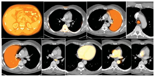
Sample recognition results for Thorax for the alignment strategy shown in (10). Cross sections of the model are shown overlaid on test image slices. Left to right: TSkn, TSk, LPS, TB, RPS, E, PC, AS, VS.

Figure 8.

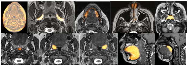
Sample recognition results for Neck for the alignment strategy shown in (10). Cross sections of the model are shown overlaid on test image slices. Left to right: NSkn, FP, Mnd, NP (note that NP is a combination of nasal cavity and nasopharynx), Ad, OP, RT, LT, Tng, SP.

Table 6.

Recognition results (mean, standard deviation) for Thorax for the strategy in (10). (“Mean” excludes VS.)

	TSkn	RS	TSk	IMS	LPS	TB	RPS	E	PC	AS	VS	Mean
Location Error (mm)	3.9	5.5	9.0	5.6	6.3	11.6	10.4	9.8	8.6	10.7	31.8	8.1
	1.5	2.3	5.0	3.5	3.1	5.0	4.7	4.8	5.0	5.4	12.0	4.0
Size error	1.0	0.99	0.96	0.95	0.97	0.91	0.98	0.9	0.95	1.01	0.77	0.96
	0.01	0.02	0.05	0.05	0.03	0.06	0.04	0.14	0.05	0.08	0.06	0.06

Table 9.

Recognition results for Thorax with no orientation alignment. (“Mean” excludes VS.)

	TSkn	RS	TSk	IMS	LPS	TB	RPS	E	PC	AS	VS	Mean
Location Error (mm)	3.9	5.5	9	5.6	6.3	8	10.4	14.2	8.6	8.1	33.6	8.0
	1.5	2.3	5	3.5	3.1	6.5	4.7	10.5	5	7.5	15.1	4.9
Size error	1.01	0.99	0.96	0.95	0.97	0.83	0.98	0.85	0.95	0.99	0.77	0.95
	0.01	0.02	0.05	0.05	0.03	0.08	0.04	0.12	0.05	0.08	0.06	0.05

Table 8.

Recognition results (mean, standard deviation) for Neck for the strategy in (10).

	NSkn	A&B	FP	NSTs	Mnd	Phrx	Tnsl	Tng	SP	Ad	NP	OP	RT	LT	Mean
Location Error(mm)	3	7.8	4.2	4.8	12.5	10.4	2.8	4.9	5.1	1.8	11.1	10	2.9	2.3	5.96
	1.2	3.8	2.1	2.1	3.7	4.5	1.8	2.8	1.8	0.8	6.8	8.7	2.2	2.1	1.96
Size error	1	0.9	1	0.92	0.74	0.8	1	1.02	0.93	0.9	0.65	0.74	0.92	0.9	0.93
	0.01	0.03	0.03	0.06	0.05	0.04	0.1	0.06	0.24	0.12	0.07	0.2	0.11	0.12	0.04

$$\begin{array}{l}\text{Non}-\text{sparse}\&\text{hybrid}\text{objects}:\text{RS},\text{LPS},\text{RPS},\text{IMS},\text{TSk},\text{Ask},\text{Kd},\text{Spl},\text{Msl},\text{LKd},\text{RKd},\mathrm{A}\&\mathrm{B},\text{FP},\\ \text{NSTs},\text{Mnd},\text{Tnsl},\text{Tng},\text{SP},\text{Ad},\text{RT},\text{LT}-\text{no}\text{orientation}\text{alignment}.\\ \text{Sparse}\text{objects}:\text{TB},\mathrm{E},\text{AS},\text{VS},\text{AIA},\text{IVC},\text{Phrx},\text{NP},\text{OP}-\text{orientation}\text{alignment}\text{by}\text{all}\text{axes}.\end{array}$$ (10)

The recognition accuracy is expressed in terms of position and size. The position error is defined as the distance between the geometric centers of the known true objects in I^b and the center of the adjusted fuzzy model FM^T(O_l). The size error is expressed as a ratio of the estimated size of the object at recognition and true size. Values 0 and 1 for the two measures, respectively, indicate perfect recognition. Note in Figures 6–8 that the model bleeds into adjacent tissue regions with some membership value since it is fuzzy. This should not be construed as wrong segmentation. The main issue is if the model placement via recognition is accurate enough to yield good delineation. Similarly and due to the slice visualization mode, sparse object components may appear to be missed or to present with low membership values.

Although we have not conducted extensive experiments to test all possible arrangements for orientation alignment for non-sparse and sparse objects, generally we found that orientation adjustment for non-sparse objects does not improve recognition results. In some cases like PC, it may actually lead to deterioration of results. In our experience, the set up in (10) turned out to be an excellent compromise from the viewpoint of accuracy of results and efficiency. For comparison, we demonstrate in Table 9 recognition results for the thorax with no orientation adjustment for any object in both model building and recognition.

Size error is always close to 1 for all body regions and objects. Generally, recognition results for non-sparse objects are excellent with a positional error of mostly 1–2 voxels. Note that for DS1 and DS2, voxels are quite large¹¹. We observed that, the positional accuracy within the slice plane is better than across slices. In other words, errors listed in the tables are mostly in the third dimension in which voxel size is large. Orientation adjustment improves recognition somewhat for some sparse objects, but has negligible effect for non-sparse objects, at least in the thorax.

The recognition results for the MRI data set DS4 are demonstrated in Figure 9 and Table 10. Again, since the model is fuzzy, it will encroach into adjacent tissue regions with some membership value. Since our goal here was just to measure subcutaneous adiposity, the hierarchy was simplified as shown in Figure 9. Again the position error is 1–2 voxels. These results are particularly noteworthy since they are generated by using the models built from image data sets acquired from a different modality, namely CT, and for a different group with an age difference of about 40 years and with a different gender. This underscores the importance of understanding the dichotomy between recognition and delineation. Recognition is a high-level and rough process which gives anatomic context. The models do not have to be, and we argue should not be, detailed attempting to capture fine details. Obtaining the anatomic context is a necessary step for achieving accurate delineation. It is important to note here that for the cross modality operation to work in this manner, the MR image intensities must be standardized (Nyul and Udupa 1999).

Figure 9.

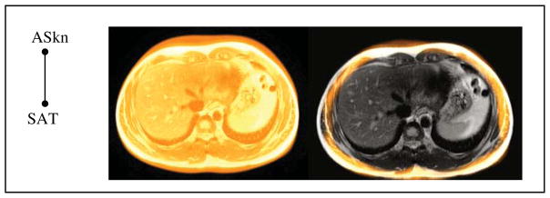
The hierarchy used (left) and sample recognition results for DS4 (right) with model cross section overlaid on test image slices for ASkn and SAT.

Table 10.

Recognition accuracy for the objects shown in Figure 9.

	ASkn	SAT
Position Error (mm)	4.6	12.97
	2.5	5.3
Size Error	1.01	1
	0.05	0.03

5.4 Object delineation

Sample delineation results are displayed in Figures 10–13 for DS1–DS4. Delineation accuracy statistics for these data sets, expressed as false positive and false negative volume fractions (FPVF, FNVF) as well as mean Hausdorff distance (HD) between the true and delineated boundary surfaces, are listed in Tables 11–14. The HD measure is defined as the mean over all test subjects of the median of the distances of the points on the delineated object boundary surface from the true object boundary surface.

Figure 10.

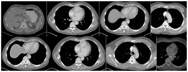
Sample delineation results for Thorax. Left to Right: TSkn, IMS, LPS, AS, RPS, PC, TB, E.

Figure 13.

Sample delineation results for DS4. ASkn (left) and SAT (right).

Table 11.

Delineation results for Thorax (mean & standard deviation).

	TSkn	RS	TSk	IMS	LPS	RPS	E	PC	TB	AS
FPVF	0.02	0.0	0.19	0.03	0.01	0.01	0.0	0.01	0.01	0.01
	0.02	0.0	0.05	0.01	0.03	0.02	0.0	0.00	0.00	0.00
FNVF	0.05	0.06	0.13	0.07	0.04	0.04	0.49	0.09	0.16	0.17
	0.06	0.04	0.07	0.07	0.02	0.02	0.19	0.06	0.14	0.17
HD (mm)	3.6	1.24	10.6	6.2	2.9	2.1	3.1	3.5	5.2	5.3
	4.5	0.42	2.4	1.8	8.8	4.7	0.87	1.3	1.8	2.5

Table 14.

Delineation results for DS4.

	ASkn	SAT
FPVF	0.0	0.06
FNVF	0.03	0.01
HD (mm)	1.7	3.9

Delineation results for VS (Thorax) are not presented since the recognition accuracy for VS is not adequate for reliable delineation. We note that the delineation of 21 non-sparse objects achieves a mean FPVF and FNVF of 0.02 and 0.08, respectively, and a mean HD of 0.9 voxels, which are generally considered to be excellent. Six sparse objects also achieve good delineation outcome, with the above mean measures reading 0.05, 0.15, and 1.5, respectively. However, sparse objects VS, E, IVC, Mnd, and NP pose challenges for effective delineation. Often, even when their recognition is effective, it is difficult to guarantee placement of seed sets A_O and A_B appropriately within and outside these objects because of their sparse nature. In DS3 (MR images of neck), it is very difficult to properly delineate Mnd, NP, and OP because of their poor definition in the image. To test the effectiveness of the models created from these data (DS3) in segmenting the same objects on CT data of a group of three different pediatric subjects, we devised a simple hierarchy with NSkn as the root and with Mnd, NP, and OP as its offspring objects. The delineation results obtained for these four objects were excellent, with a mean FPVF of 0, 0.01, 0, and 0.02, and mean FNVF of 0.01, 0.01, 0.02 and 0.1, respectively.

5.5 Comparison with a non-hierarchical approach

To study the effect of the hierarchy and the knowledge encoded in it on recognition, we list in Table 15 the recognition performance of a non-hierarchical approach. The results are shown for Thorax wherein each object is recognized on its own by using the same fuzzy models FM(O_l) as used in the hierarchical AAR system. The initial pose for search is taken to be the center of the image and search range covers roughly the whole body region with the scale factor range the same as that for the hierarchical approach. In comparison to the hierarchical approach (Tables 6 and 9), it is clear that non-hierarchical recognition performance is much worse.

Table 15.

Recognition results for Thorax: non-hierarchical approach (mean & standard deviation).

	TSkn	RS	TSk	IMS	LPS	TB	RPS	E	PC	AS	VS	Mean
Location error (mm)	10.5	12.9	21.1	27.7	91.4	53.3	72.3	42.4	45.5	23.1	82.2	43.8
	9.5	13.1	21.8	9.8	10.8	20.9	12.9	34.5	12.5	15.2	33.8	17.7
Size error	1.0	1.01	0.96	0.92	0.8	0.82	0.8	0.86	0.9	0.97	0.81	0.9
	0.02	0.09	0.08	0.07	0.09	0.06	0.07	0.14	0.06	0.11	0.08	0.08

5.6 Computational considerations

Program execution times are estimated on a Dell computer with the following specifications: 4-core Intel Xeon 3.6 GHz CPU with 8 GB RAM and running the Linux-jb18 3.7.10–1.16 operating system. Mean computational times for the AAR steps are listed in Table 16. Model building includes the construction of fuzzy models and the estimation of ρ, λ, and all parameters related to recognition and delineation, including the optimal threshold parameters Th_l. This latter step takes about 12 seconds per object. As seen from Table 16, each of the three main operations takes under 1 minute per object. Among these operations, only the time for model building depends on the number of training data sets, while recognition and delineation are independent of this factor. On average, model building times per object per training data set for Thorax, Abdomen, and Neck are, respectively, 1.4 sec, 1.7 sec, and 1 sec. In statistical atlas based methods, the computational time for image registration becomes the bottleneck. Our calculation taking Elastix as a representative registration tool kit (Klein et al. 2010) indicates that the creation of a single atlas for each of the 11 objects of the Thorax at a reduced image resolution of 2.5 × 2.5 × 2.5 mm³ for the 25 training data sets of DS1 would take about 23.5 hours compared to 6.4 min for the AAR system. The time per object for recognition and delineation can also take several minutes for these methods. Even with 100 data sets for training and 15 objects in a body region, the total time needed for the AAR model building step would be about 40 minutes, whereas atlas building may take days to complete especially when multi-atlas strategies are used.

Table 16.

Mean computational time in seconds per object for different operations and body regions.

Operation	Thorax	Abdomen	Neck
Model building	35	42	24
Object recognition	30	46	6
Object delineation	47	56	24

5.7 Comparison with other methods

The publications reporting works that are directly related to our work in spirit are (Baiker et al. 2010, Chu et al. 2013, Criminisi et al. 2013, Lu et al. 2012, Linguraru et al. 2012, Okada et al. 2008, Zhou et al. 2012). In Table 17, we present a comparison to our AAR system based on the results reported in these works. We note that a quantitative grading/understanding of the methods is impossible since the data sets used, acquisition protocols and resolutions, considered objects, training and test data set subdivisions, cross validation strategies, and computing platforms are all different in these methods. Interestingly, a commonality among them is that they all focused on CT image data sets.

Table 17.

A comparison with the current methods from the literature that are related to our work. Unknown and irrelevant entries are indicated by “~”.

Method	Objects	Voxel size (mm3)	Training-to-test data proportion	Location error (mm)	Region overlap (Dice, Jackard Index (JI), etc.)
Lu et al. 2012	Prostate, bladder, rectum	~ × ~ × 0.8 to 5	141 to 47, 4-fold	2.4 to 4.2	~
Linguraru et al. 2012	Liver, spleen, kidneys	(0.5 to 0.9)2 × 1 to 5	27 to 1, 28-fold	0.8 to 1.2	90.9% to 94.8%
Okada et al. 2008	Liver, vena cava, gallbladder	0.7 × 0.7 × 2.5	20 to 8	(for liver) 1.5 to 2.8	88%
Chu et al. 2013	Liver, spleen, pancreas, kidneys	(0.55 to 0.82)2 × 0.7 to 1 (estimated)	90 to 10, 10-fold	~	56% (pancreas-JI) to 95.2% (liver-Dice)
Criminisi et al. 2013	26 anatomic structures in the torso	(0.5 to 1)2 × 1 to 5	318 to 82	9.7 to 19.1 (mean for each structure)	~
Zhou et al. 2012	12 organ regions in thorax, abdomen, pelvis	(0.6 to 0.7)3	300 to 1000	6 to 14 for mode locations	~
Baiker et al. 2010	Brain, heart, kidneys, lungs, liver, skeleton	(0.332)3	MOBY atlas, 26 datasets	~	47% to 73%

Among these methods, (Chu et al. 2013, Linguraru et al. 2012, Lu et al. 2012, Okada et al. 2008) comprise one group wherein the body region of focus was the pelvis or abdomen, with 3–5 objects considered for segmentation. They all employ an object localization step, which is achieved either through an atlas (Chu et al. 2013, Linguraru et al. 2012, Okada et al. 2008), statistical shape models (Okada et al. 2008), or machine learning techniques (Lu et al. 2012), and subsequently a delineation step that uses graph cuts (Chu et al. 2013, Linguraru et al. 2012), information theory (Lu et al. 2012), and MAP or ML estimation (Chu et al. 2013, Okada et al. 2008). In the second group (Criminisi et al. 2013, Zhou et al. 2012), the aim is only to locate the objects via machine learning techniques. The third group is constituted by (Baiker et al. 2010), the only work that considered body-wide organs, but in mice, using a kinematic model of the skeletal joints to localize objects relative to different skeletal components.

We observe that, for the same objects (liver, kidneys, and spleen), our results are comparable to, often better than, the current results from literature, especially considering the 5 mm slice spacing and the equal training-to-test data set proportion for our evaluation. We conclude that the development of a general AAR system that can be readily applied and adapted to different body regions, multitudes of organs, and modalities has not yet been demonstrated. Perhaps some of the above methods can be made to work in this general manner. However, we believe that this may require considerable further development and innovation.

6. CONCLUDING REMARKS

In this paper, we presented a general body of methods for automatic anatomy recognition and delineation whose principles are not tied to any specific body region, organ system, or imaging modality. We took a fuzzy approach for building the models and attempted to harness as much specific anatomic information as possible to be embedded into the fuzzy anatomic model. We demonstrated the generality of the approach by examining the performance of the same AAR system on three different body regions using CT and MR image data sets. We also illustrated the potential of the system for rapid prototyping by demonstrating its adaptability to a new application on a different modality (DS4). Our system is set up to operate fully automatically. All image modality-specific parameters needed – threshold intervals for objects in for recognition and affinity parameters for delineation – are estimated automatically from the training data sets. When a new application is sought at a modality different from those considered in the anatomy model FAM( , G), a few sample segmentations of the objects of interest and the matching images are needed for relearning these image intensity-related parameter values (specifically, Th_l and the affinity parameters). All other modality-independent aspects of the model do not need retraining. In the case of MRI, images from each separate MRI protocol have to be standardized for image intensity so that setting up these parametric values becomes sensible. Separation of modality-independent from dependent aspects, organization of objects in a hierarchy, encoding object relationship information into the hierarchy, optimal threshold-based recognition learning, and fuzzy model-based IRFC are novel and powerful concepts with consequences in recognition and delineation, as we demonstrated in this paper.

While the above strengths of this AAR system are quite unique as revealed in our literature review, the system has some limitations at present. First, we have not studied the performance of the system on patient images that contain significant pathology. However, we note that DS4 indeed includes image data sets of patients who are obese. Note also that these image data sets are from a very different age and gender group and on a different imaging modality from those used to build FAM( , G). We believe that it is essential to make the system operate satisfactorily on normal or near-normal images before testing it on images with diverse pathologies. As such, we are currently in the process of testing the system on organs and organ systems with significant pathology in all three body regions focusing on specific disease processes.

Second, the accuracy is inadequate for some sparse objects for recognition (VS, IVC) and delineation (E, Mnd, NP). Also we have not considered in this paper other important and challenging sparse objects such as the adrenal glands, pancreas, and the spinal cord. If recognition is inadequate, delineation will become unacceptable because it becomes impossible to appropriately initialize the delineation process and to exploit the model for making up for missing boundary information in the image in delineation. When we closely examined these cases, it became clear that there are fundamental challenges in the model building stage itself for sparse objects. Generally we found that sparse objects have much greater variation than their non-sparse counterparts in form, topology, and geographic layout, compared to their size. As an example, consider AS and VS (Thorax). The descending aortic portion of AS is often straight and directed vertically downward while in some subjects it may be inclined, curved, or even tortuous, with other portions, especially the aortic arch, not varying much. The branching pattern of the left and right brachiocephalic veins and the course of the azygos vein in VS also vary considerably. In view of such difficulties, we have come to the realization that sparse objects should not be modeled directly from their precise shape information in the binary image set I^b, instead only their rough super form (such as a minimal super set that subsumes such variations) should be utilized in model building. We are exploring the use of rough sets (Maji and Pal 2012) for this purpose.

The AAR methodology seems to have definite computational advantages over atlas-based approaches. Further, in atlas-based methods, it is perhaps much more challenging to incorporate the extensive object-level knowledge that the AAR approach exploits at various stages for recognition and delineation. These incorporations constitute highly non-linear and discontinuous phenomena which are effected in intensity, geometric, and topological spaces. The kinematic model employed in (Baiker et al. 2010) is a good analogy of how one may encode object relationships via a model that are difficult to emulate through continuous and smooth image/atlas deformations.

Some of the avenues we are currently exploring for the proposed AAR approach are delineated below.

In this paper, we did not address the problem of automatically determining the body region following the definition of within the given data set. As demonstrated in (Chen et al. 2012), it is possible to determine the slices delimiting a body region automatically based on slice profiles. Furthermore, the information about the relationship between and WB can also be encoded into the hierarchy as illustrated in Figure 2(a) for each .

The use of composite objects often leads to better recognition accuracy. This is because the multiple objects contained in a composite object offer tighter constraints in recognition search. The aspect of how objects can be grouped to achieve optimum recognition results needs investigation. A related topic is how to device optimal hierarchies for a given body region. The hierarchies we have considered so far are anatomically motivated. Perhaps there are “optimal” hierarchies from the view point of achieving the best recognition (and hence, delineation) results. In such an investigation, matters of how objects should be grouped as well as ordered in the hierarchy can both be addressed simultaneously using graph optimization techniques.

We have set up the AAR-R and AAR-D procedures in a general way. Recognition and delineation algorithms other than those we have tested can be used independently for R-ROOT and R-OBJECT and for D-ROOT and D-OBJECT within the same hierarchical set up. Similar to composite object recognition, delineation done simultaneously for multiple objects, unlike the one-object-at-a-time approach of AAR-D, may improve overall accuracy.

Computationally, there are three expensive operations in the AAR system – image interpolation, distance transform, and the delineation algorithm (FMIRFC). To make recognition and delineation operate in practical time in a clinical setting, implementations of these operations will have to be sped up. Toward this goal, we are studying GPU implementations of these operations. GPU implementations of some fuzzy connectedness algorithms have already been published (Zhuge et al. 2011, Zhuge et al. 2013).

Finally, along the lines of the study underlying DS4, we are exploring the adaptation of the AAR system to several clinical applications.

Figure 7.

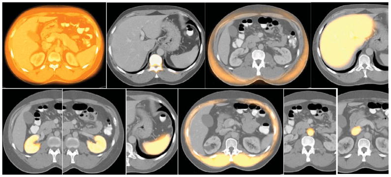
Sample recognition results for Abdomen for the alignment strategy shown in (10). Cross sections of the model are shown overlaid on test image slices. Left to right: ASkn, ASk, SAT, Lvr, RKd, LKd, Spl, Msl, AIA, IVC.

Figure 11.

Sample delineation results for Abdomen. Left to Right: ASkn, SAT, Lvr, SAT, RKd, LKd, Spl, Msl, AIA.

Figure 12.

Sample delineation results for Neck. Left to Right: NSkn, FP, NP, OP, RT, LT, Tng, SP, Ad.

Table 4.

Size correlation among objects of the Abdomen.

	ASkn	ASk	ASTs	Lvr	SAT	Msl	Spl	RKd	LKd	AIA	IVC
ASkn	1
ASk	0.68	1
ASTs	0.9	0.8	1
Lvr	0.61	0.48	0.58	1
SAT	1	0.69	0.92	0.61	1
Msl	0.91	0.79	0.99	0.63	0.94	1
Spl	0.62	0.43	0.61	0.51	0.65	0.62	1
RKd	0.53	0.64	0.57	0.61	0.51	0.6	0.34	1
LKd	0.53	0.56	0.52	0.51	0.49	0.54	0.34	0.87	1
AIA	0.6	0.85	0.7	0.27	0.58	0.68	0.49	0.51	0.5	1
IVC	0.32	0.58	0.47	0.29	0.32	0.46	0.3	0.38	0.36	0.67	1

Table 7.

Recognition results (mean, standad deviation) for Abdomen for the strategy in (10).

	ASkn	SAT	ASk	Lvr	ASTs	Kd	Spl	Msl	AIA	IVC	RKd	LKd	Mean
Location Error(mm)	5.9	20.2	11.7	7.9	7.2	10.6	11.6	7.7	8.2	8.7	11.3	7.3	9.8
	3.4	8.5	7.9	5.4	3.0	9.8	13.9	3.6	2.8	7.2	11.6	7.4	7
Size error	1.0	0.97	0.96	0.93	1.0	0.94	1.2	1.01	1.1	1.15	0.97	0.93	1.01
	0.02	0.03	0.06	0.07	0.02	0.09	0.19	0.03	0.13	0.1	0.1	0.08	0.07

Table 12.

Delineation results for Abdomen (mean & standard deviation).

	Askn	ASk	Lvr	ASTs	SAT	RKd	LKd	Spl	Msl	AIA
FPVF	0.01	0.06	0.04	0.12	0.05	0.00	0.01	0.0	0.13	0.01
	0.00	0.01	0.02	0.05	0.03	0.00	0.01	0.0	0.03	0.0
FNVF	0.05	0.14	0.1	0.15	0.12	0.13	0.1	0.13	0.09	0.13
	0.08	0.09	0.05	0.09	0.02	0.04	0.02	0.03	0.08	0.03
HD (mm)	1.7	6.9	5.3	1.74	1.6	2.4	5.4	6.8	2.5	5.6
	2.7	1.5	1.6	1.0	0.8	1.1	4.8	6.0	1.1	1.8

Table 13.

Delineation results for Neck (mean & standard deviation).

	NSkn	FP	Mnd	NP	OP	RT	LT	Tng	SP	Ad
FPVF	0.0	0.0	0.01	0.01	0.0	0.01	0.01	0.02	0.01	0.0
	0.0	0.0	0.0	0.0	0.0	0.0	0.0	0.01	0.01	0.0
FNVF	0.0	0.1	0.49	0.32	0.2	0.06	0.06	0.02	0.08	0.07
	0.01	0.05	0.08	0.2	0.02	0.02	0.01	0.01	0.01	0.04
HD (mm)	2.8	0.83	3.3	3.8	7.6	3.3	3.2	8.4	8.03	2.2
	0.06	0.53	0.56	1.01	2.4	0.62	1.4	1.92	4.0	0.3

HIGHLIGHTS.

• Fuzzy hierarchical modeling of all major organs in a body region

• Detailed object relationship information encoded into models

• Hierarchical object recognition and delineation

• Optimal threshold-based recognition strategy

• Demonstration of the same method on several body regions and different modalities

APPENDIX

Table 1.

Anatomic definitions of organs considered in this paper.

Thoracic objects	Acronym	Definition of object
Thoracic skin	TSkn	The outer boundary of the thoracic skin (arms excluded). The interior region constitutes the entire thoracic body region. The inferior boundary is defined to be 5 mm below the base of the lungs and the superior boundary is defined to be 15 mm above the lung apices.
Thoracic skeleton	TSk	All skeletal structures contained in the thoracic body region, including the spine, ribs, sternum, and the portions of the scapulae and clavicles that are inside the body region.
Respiratory system	RS	Grouping of RPS, LPS, and TB.
Right lung	RPS	The outer boundary of the right lung along the right pleura.
Left lung	LPS	The outer boundary of the left lung along the left pleura.
Trachea and bronchi	TB	The outer boundary of the trachea and bronchi from the superior thoracic trachea to the distal main stem bronchi.
Internal mediastinum	IMS	Grouping of PC, E, AS, and VS.
Pericardial region	PC	Region within the boundary of pericardial sac. The superior aspect is defined by the branching of the main pulmonary artery.
Esophagus	E	The outer boundary of the esophagus from the superior aspect of thorax to the level of gastric cardia.
Arterial system	AS	The outer boundary of the ascending aorta, aortic arch, descending thoracic aorta, pulmonary arteries, innominate artery, proximal left common carotid artery, and proximal left subclavian artery. The superior aspect is defined by the branching of the innominate artery.
Venous system	VS	The outer boundary of the superior vena cava, right and left brachiocephalic veins, and azygos vein.
Abdominal objects	Acronym	Definition of object
Abdominal skin	ASkn	The outer boundary of the abdominal skin. The interior region constitutes the entire abdominal body region. The superior boundary is defined by the superior aspect of the liver. The inferior boundary is defined by the bifurcation of the abdominal aorta into the common iliac arteries.
Abdominal skeleton	ASk	All skeletal structures contained in the abdominal body region, including lumbar spine and portion of the inferior ribs within the body region.
Soft tissue	ASTs	Grouping of Kd, Spl, Msl, AIA, IVC.
Kidneys	Kd	Grouping of RKd and LKd.
Right kidney	RKd	The outer boundary of the right kidney. All external blood vessels are excluded.
Left kidney	LKd	The outer boundary of the left kidney. All external blood vessels are excluded.
Spleen	Spl	The outer boundary of the spleen. All external blood vessels are excluded
Muscle	Msl	The outer boundaries of the abdominal musculature, including the rectus abdominis, abdominal oblique, psoas, and paraspinal muscles.
Abdominal aorta	AIA	The outer boundary of the abdominal aorta. The superior and inferior slices of AIA are the same as those of the abdominal region.
Inferior vena cava	IVC	The outer boundary of the inferior vena cava. The superior and inferior slices of IVC are the same as those of the abdominal region.
Liver	Lvr	The outer boundary of the liver. The intrahepatic portal veins and hepatic arteries are included in this region.
Fat	Fat	Grouping of SAT and VAT.
Subcutaneous adipose tissue	SAT	Adipose tissue in the subcutaneous region in the abdomen.
Visceral adipose tissue	VAT	Adipose tissue internal to the abdominal musculature.
Neck objects	Acronym	Definition of object
Head and Neck skin	NSkn	The outer boundary of the head and neck skin, where the interior region constitutes the entire head and neck body region. The superior boundary is defined by a level 6.6 mm above the superior aspect of the globes. The inferior boundary is defined by a level 6.6 mm inferior to the inferior aspect of the mandible.
Air and Bone	A&B	Grouping of Mnd and Phrnx.
Mandible	Mnd	The outer boundary of the mandible.
Pharynx	Phrx	Grouping of NP and OP.
Nasopharyngeal airway	NP	The outer contour of the nasal and nasopharyngeal air cavity, extending to the inferior aspect of the soft palate.
Oropharyngeal airway	OP	The outer contour of the oropharyngeal air cavities, extending from the inferior aspect of the soft palate to the superior aspect of the epiglottis.
Fat pad	FP	The outer boundary of the parapharyngeal fat pad.
Neck soft tissues	NSTs	Grouping of Tnsl, Tng, SP, Ad.
Palatine tonsils	Tnsl	Grouping of RT and LT.
Right palatine tonsil	RT	The outer boundary of the right palatine tonsil.
Left palatine tonsil	LT	The outer boundary of the left palatine tonsil.
Tongue	Tng	The outer boundary of the tongue.
Soft palate	SP	The outer boundary of the soft palate.
Adenoid tissue	Ad	The outer boundary of the adenoid tissue.

References

- Arens R, Sin S, Nandalike K, Rieder J, Khan UI, Freeman K, Wylie-Rosett J, Lipton ML, Wootton DM, McDonough JM, Shifteh K. Upper Airway Structure and Body Fat Composition in Obese Children with Obstructive Sleep Apnea Syndrome. American Journal of Respiratory and Critical Care Medicine. 2011;183:782–787. doi: 10.1164/rccm.201008-1249OC. [DOI] [PMC free article] [PubMed] [Google Scholar]
- Ashburner J, Friston KJ. Computing average shaped tissue probability templates. Neuroimage. 2009;45:333–341. doi: 10.1016/j.neuroimage.2008.12.008. [DOI] [PubMed] [Google Scholar]
- Baiker M, Milles J, Dijkstra J, Henning TD, Weber AW, Que I, Kaijzel EL, Lowik CWGM, Reiber JHC, Lelieveldt BPF. Atlas-based whole-body segmentation of mice from low-contrast Micro-CT data. Medical Image Analysis. 2010;14:723–737. doi: 10.1016/j.media.2010.04.008. [DOI] [PubMed] [Google Scholar]
- Beucher S. The Watershed Transformation applied to image segmentation. 10th Pfefferkorn Conference on Signal and Image Processing in Microscopy and Microanalysis; 1992. pp. 299–314. [Google Scholar]
- Bogovic JA, Prince JL, Bazin PL. A multiple object geometric deformable model for image segmentation. Computer Vision and Image Understanding. 2013;117:145–157. doi: 10.1016/j.cviu.2012.10.006. [DOI] [PMC free article] [PubMed] [Google Scholar]
- Boykov Y, Veksler O, Zabih R. Fast approximate energy minimization via graph cuts. IEEE Transactions on Pattern Analysis and Machine Intelligence. 2001;23:1222–1239. [Google Scholar]
- Cabezas M, Oliver A, Llado X, Freixenet J, Cuadra MB. A review of atlas-based segmentation for magnetic resonance brain images. Comput Methods Programs Biomed. 2011;104:158–177. doi: 10.1016/j.cmpb.2011.07.015. [DOI] [PubMed] [Google Scholar]
- Cerrolaza JJ, Villanueva A, Cabeza R. Hierarchical Statistical Shape Models of Multiobject Anatomical Structures: Application to Brain MRI. IEEE Transactions on Medical Imaging. 2012;31:713–724. doi: 10.1109/TMI.2011.2175940. [DOI] [PubMed] [Google Scholar]
- Chen XJ, Bagci U. 3D automatic anatomy segmentation based on iterative graph-cut-ASM. Medical Physics. 2011;38:4610–4622. doi: 10.1118/1.3602070. [DOI] [PMC free article] [PubMed] [Google Scholar]
- Chen XJ, Udupa JK, Bagci U, Zhuge Y, Yao J. Medical image segmentation by combining graph cut and oriented active appearance models. IEEE Transactions on Image Processing. 2012;21(4):2035–2046. doi: 10.1109/TIP.2012.2186306. [DOI] [PMC free article] [PubMed] [Google Scholar]
- Chu C, Oda M, Kitasaka T, Misawa K, Fujiwara M, Hayashi Y, Wolz R, Rueckert D, Mori K. Multi-organ segmentation from 3D abdominal CT images using patient-specific weighted-probabilistic atlas. SPIE Medical Imaging. SPIE; 2013. pp. 86693Y-86691–86693Y-86697. [Google Scholar]
- Ciesielski KC, Udupa JK, Falcao AX, Miranda PAV. Fuzzy Connectedness Image Segmentation in Graph Cut Formulation: A Linear-Time Algorithm and a Comparative Analysis. Journal of Mathematical Imaging and Vision. 2012;44:375–398. [Google Scholar]
- Cootes TF, Edwards GJ, Taylor CJ. Active appearance models. IEEE Transactions on Pattern Analysis and Machine Intelligence. 2001;23:681–685. [Google Scholar]
- Criminisi A, Robertson D, Konukoglu E, Shotton J, Pathak S, White S, Siddiqui K. Regression forests for efficient anatomy detection and localization in computed tomography scans. Med Image Anal. 2013;17:1293–1303. doi: 10.1016/j.media.2013.01.001. [DOI] [PubMed] [Google Scholar]
- Duta N, Sonka M. Segmentation and interpretation of MR brain images: An improved active shape model. IEEE Transactions on Medical Imaging. 1998;17:1049–1062. doi: 10.1109/42.746716. [DOI] [PubMed] [Google Scholar]
- Hansegard J, Urheim S, Lunde K, Rabben SI. Constrained active appearance models for segmentation of triplane echocardiograms. IEEE Transactions on Medical Imaging. 2007;26:1391–1400. doi: 10.1109/TMI.2007.900692. [DOI] [PubMed] [Google Scholar]
- Heimann T, Meinzer HP. Statistical shape models for 3D medical image segmentation: A review. Medical Image Analysis. 2009;13:543–563. doi: 10.1016/j.media.2009.05.004. [DOI] [PubMed] [Google Scholar]
- Horsfield MA, Bakshi R, Rovaris M, Rocca MA, Dandamudi VSR, Valsasina P, Judica E, Lucchini F, Guttmann CRG, Sormani MP, Filippi M. Incorporating domain knowledge into the fuzzy connectedness framework: Application to brain lesion volume estimation in multiple sclerosis. IEEE Transactions on Medical Imaging. 2007;26:1670–1680. doi: 10.1109/tmi.2007.901431. [DOI] [PubMed] [Google Scholar]
- Kass M, Witkin A, Terzopoulos D. Snakes - Active Contour Models. International Journal of Computer Vision. 1987;1:321–331. [Google Scholar]
- Klein S, Staring M, Murphy K, Viergever MA, Pluim JPW. Elastix: a toolbox for intensity based medical image registration. IEEE Transactions on Medical Imaging. 2010;29:196–205. doi: 10.1109/TMI.2009.2035616. [DOI] [PubMed] [Google Scholar]
- Linguraru MG, Pura JA, Pamulapati V, Summers RM. Statistical 4D graphs for multi-organ abdominal segmentation from multiphase CT. Med Image Anal. 2012;16:904–914. doi: 10.1016/j.media.2012.02.001. [DOI] [PMC free article] [PubMed] [Google Scholar]
- Liu JM, Udupa JK. Oriented Active Shape Models. IEEE Transactions on Medical Imaging. 2009;28:571–584. doi: 10.1109/TMI.2008.2007820. [DOI] [PubMed] [Google Scholar]
- Lu C, Zheng Y, Birkbeck N, Zhang J, Kohlberger T, Tietjen C, Boettger T, Duncan JS, Zhou SK. Precise segmentation of multiple organs in CT volumes using learning-based approach and information theory. Med Image Comput Comput Assist Interv. 2012;15:462–469. doi: 10.1007/978-3-642-33418-4_57. [DOI] [PubMed] [Google Scholar]
- Maji P, Pal SK. Rough-Fuzzy Pattern Recognition: Applications in Bioinformatics and Medical Imaging. John Wiley & Sons, Inc; New York: 2012. [Google Scholar]
- Malladi R, Sethian JA, Vemuri BC. Shape Modeling with Front Propagation - a Level Set Approach. IEEE Transactions on Pattern Analysis and Machine Intelligence. 1995;17:158–175. [Google Scholar]
- Maurer CR, Qi RS, Raghavan V. A linear time algorithm for computing exact Euclidean distance transforms of binary images in arbitrary dimensions. IEEE Transactions on Pattern Analysis and Machine Intelligence. 2003;25:265–270. [Google Scholar]
- Meyer C, Peters J, Weese J. Fully automatic segmentation of complex organ systems: Example of trachea, esophagus and heart segmentation in CT images. SPIE Medical Imaging SPIE. 2011:796216-796211–796216-796211. [Google Scholar]
- Miranda PAV, Falcao AX, Udupa JK. Clouds: A model for synergistic image segmentation. ISBI. 2008:209–212. [Google Scholar]
- Miranda PAV, Falcao AX, Udupa JK. Cloud Bank: A multiple clouds model and its use in MR brain image segmentation. ISBI. 2009:506–509. [Google Scholar]
- Mumford D, Shah J. Optimal Approximations by Piecewise Smooth Functions and Associated Variational-Problems. Communications on Pure and Applied Mathematics. 1989;42:577–685. [Google Scholar]
- Nyul LG, Udupa JK. On standardizing the MR image intensity scale. Magnetic Resonance in Medicine. 1999;42:1072–1081. doi: 10.1002/(sici)1522-2594(199912)42:6<1072::aid-mrm11>3.0.co;2-m. [DOI] [PubMed] [Google Scholar]
- Okada T, Yokota K, Hori M, Nakamoto M, Nakamura H, Sato Y. Construction of hierarchical multi-organ statistical atlases and their application to multi-organ segmentation from CT images. Med Image Comput Comput Assist Interv. 2008;11:502–509. doi: 10.1007/978-3-540-85988-8_60. [DOI] [PubMed] [Google Scholar]
- Pizer SM, Fletcher PT, Joshi S, Thall A, Chen JZ, Fridman Y, Fritsch DS, Gash AG, Glotzer JM, Jiroutek MR, Lu CL, Muller KE, Tracton G, Yushkevich P, Chaney EL. Deformable M-reps for 3D medical image segmentation. International Journal of Computer Vision. 2003;55:85–106. doi: 10.1023/a:1026313132218. [DOI] [PMC free article] [PubMed] [Google Scholar]
- Raya SP, Udupa JK. Shape-Based Interpolation of Multidimensional Objects. IEEE Transactions on Medical Imaging. 1990;9:32–42. doi: 10.1109/42.52980. [DOI] [PubMed] [Google Scholar]
- Rousson M, Paragios N. Prior knowledge, level set representations & visual grouping. International Journal of Computer Vision. 2008;76:231–243. [Google Scholar]
- Saha PK, Udupa JK. Relative fuzzy connectedness among multiple objects: Theory, algorithms, and applications in image segmentation. Computer Vision and Image Understanding. 2001;82:42–56. doi: 10.1016/j.cviu.2006.10.005. [DOI] [PMC free article] [PubMed] [Google Scholar]
- Shattuck DW, Mirza M, Adisetiyo V, Hojatkashani C, Salamon G, Narr KL, Poldrack RA, Bilder RM, Toga AW. Construction of a 3D probabilistic atlas of human cortical structures. Neuroimage. 2008;39:1064–1080. doi: 10.1016/j.neuroimage.2007.09.031. [DOI] [PMC free article] [PubMed] [Google Scholar]
- Shen TA, Li HS, Huang XL. Active Volume Models for Medical Image Segmentation. IEEE Transactions on Medical Imaging. 2011;30:774–791. doi: 10.1109/TMI.2010.2094623. [DOI] [PubMed] [Google Scholar]
- Souza A, Udupa JK. Iterative live wire and live snake: New user-steered 3D image segmentation paradigms. SPIE Medical Imaging SPIE. 2006:1159–1165. [Google Scholar]
- Staib LH, Duncan JS. Boundary Finding with Parametrically Deformable Models. IEEE Transactions on Pattern Analysis and Machine Intelligence. 1992;14:1061–1075. [Google Scholar]
- Torigian DA, Alavi A. The evolving role of structural and functional imaging in assessment of age-related changes in the body. Semin Nucl Med. 2007;37:64–68. doi: 10.1053/j.semnuclmed.2006.10.001. [DOI] [PubMed] [Google Scholar]
- Tsechpenakis G, Chatzis SP. Deformable probability maps: Probabilistic shape and appearance-based object segmentation. Computer Vision and Image Understanding. 2011;115:1157–1169. [Google Scholar]
- Udupa JK, Samarasekera S. Fuzzy connectedness and object definition: Theory, algorithms, and applications in image segmentation. Graphical Models and Image Processing. 1996;58:246–261. [Google Scholar]
- van der Lijn F, de Bruijne M, Klein S, den Heijer T, Hoogendam YY, van der Lugt A, Breteler MMB, Niessen WJ. Automated Brain Structure Segmentation Based on Atlas Registration and Appearance Models. IEEE Transactions on Medical Imaging. 2012;31:276–286. doi: 10.1109/TMI.2011.2168420. [DOI] [PubMed] [Google Scholar]
- Wagshul ME, Sin S, Lipton ML, Shifteh K, Arens R. Novel retrospective, respiratory-gating method enables 3D, high resolution, dynamic imaging of the upper airway during tidal breathing. Magn Reson Med. 2013 doi: 10.1002/mrm.24608. [DOI] [PMC free article] [PubMed] [Google Scholar]
- Zhou J, Rajapakse JC. Segmentation of subcortical brain structures using fuzzy templates. Neuro Image. 2005;28:915–924. doi: 10.1016/j.neuroimage.2005.06.037. [DOI] [PubMed] [Google Scholar]
- Zhou X, Yamaguchi S, Zhou X, Chen H, Hara T, Yokoyama R, Kanematsu M, Fujita H. Automatic organ localization on 3D CT images by using majority-voting of multiple 2D detections based on local binary patterns and Haar-like features. SPIE Medical Imaging SPIE. 2013:86703A-86701–86703A-86707. [Google Scholar]
- Zhou X, Wang S, Chen H, Hara T, Yokoyama R, Kanematsu M, Fujita H. Automatic localization of solid organs on 3D CT images by a collaborative majority voting decision based on ensemble learning. Computerized Medical Imaging and Graphics. 2012;36:304–313. doi: 10.1016/j.compmedimag.2011.12.004. [DOI] [PubMed] [Google Scholar]
- Zhou YX, Bai J. Atlas-based fuzzy connectedness segmentation and intensity nonuniformity correction applied to brain MRI. IEEE Transactions on Biomedical Engineering. 2007;54:122–129. doi: 10.1109/TBME.2006.884645. [DOI] [PubMed] [Google Scholar]
- Zhuge Y, Cao Y, Udupa JK, Miller RW. Parallel fuzzy connected image segmentation on GPU. Medical Physics. 2011;38(7):4365–4371. doi: 10.1118/1.3599725. [DOI] [PMC free article] [PubMed] [Google Scholar]
- Zhuge Y, Ciesielski KC, Udupa JK, Miller RW. GPU-based relative fuzzy connectedness image segmentation. Medical Physics. 2013;40 (1):011903-1–011903-10. doi: 10.1118/1.4769418. [DOI] [PMC free article] [PubMed] [Google Scholar]
- Zhuge Y, Udupa JK. Intensity standardization simplifies brain MR image segmentation. Computer, Vision and Image Understanding. 2009;113:1095–1103. doi: 10.1016/j.cviu.2009.06.003. [DOI] [PMC free article] [PubMed] [Google Scholar]