Anatomically Realistic Three-Dimensional Meshes of the Pelvic Floor & Anal Canal for Finite Element Analysis

Abstract

Three anatomically realistic meshes, suitable for finite element analysis, of the pelvic floor and anal canal regions have been developed to provide a framework with which to examine the mechanics, via finite element analysis of normal function within the pelvic floor. Two cadaver-based meshes were produced using the Visible Human Project (male and female) cryosection data sets, and a third mesh was produced based on MR image data from a live subject. The Visible Man (VM) mesh included 10 different pelvic structures while the Visible Woman and MRI meshes contained 14 and 13 structures respectively. Each image set was digitized and then finite element meshes were created using an iterative fitting procedure with smoothing constraints calculated from ‘L’-curves. These weights produced accurate geometric meshes of each pelvic structure with average Root Mean Square (RMS) fitting errors of less than 1.15 mm. The Visible Human cadaveric data provided high resolution images, however, the cadaveric meshes lacked the normal dynamic form of living tissue and suffered from artifacts related to postmortem changes. The lower resolution MRI mesh was able to accurately portray structure of the living subject and paves the way for dynamic, functional modeling.

I. Introduction

The structure of the pelvic floor and anal canal is complex and variable. Obscurity within scientific discussion has impaired the analysis and treatment of disorders in this area, and has led to confusion amongst health professionals as to the relationship of the pelvic musculature with normal defecatory function.

The motivation for this study was in recognition of the high prevalence of disorders of the rectum and anal canal and the impact disorders such as fecal incontinence and obstructed defecation can have on individuals. A recent French study revealed that over 20% of the population suffer from obstructed defecation [19]. In New Zealand it has been estimated that the incidence of some form of fecal incontinence might be as high as 15% [13], whilst estimates in the USA suggest between 2.2 and 6.9% may suffer from this disorder [5], [15]. Of most significance, fecal incontinence is a disorder that affects people of all ages. It is, however, more common in women and in older adults, but is not considered a normal part of the aging process.

Faecal incontinence occurs when the muscles in the pelvic floor lose their ability to restrict the release of rectal content from the anal canal [12] and can result from a variety of factors, such as functional impairment or structural damage to certain muscles or nerves. It is, however, rarely due to a single factor. Congenital abnormalities, such as spina bifida, can result in faecal incontinence, whilst damage to the anal sphincters from vaginal delivery, surgical procedures, inflammatory conditions or neoplastic processes can also contribute to the development or onset of faecal incontinence [20]. Medical conditions that may result in faecal incontinence include diabetes mellitus, stroke, spinal cord trauma, and degenerative disorders of the nervous system. These conditions may alter normal sensation, feedback, or function of the complex mechanism of anal continence [18].

The muscles surrounding the rectum and anal canal act to control the elimination of waste materials from the digestive tract through the process of defecation. Normal defecatory control requires the complex integration of neurological pathways and four main muscle groups in the pelvic floor and anal canal: the internal anal sphincter, external anal sphincter, puborectalis and the levator ani muscle group.

The internal anal sphincter is an involuntary smooth muscle which maintains continuous background tone and is responsible for maintaining all day continence. This muscle is a thickened distal extension of the inner circular muscle of the rectal wall [11] and responds to changing rectal pressures. The internal anal sphincter resides in the upper two thirds of the anal canal and is partially surrounded by the external anal sphincter, a powerful skeletal muscle under voluntary control. The external anal sphincter is classically divided into three sections (subcutaneous, superficialis and deep) lying adjacent to each other in series around the lower two-thirds of the anal canal [11]. The levator ani muscle group consists of three main striated muscles – pubococcygeus, iliococcygeus and puborectalis. In this study, as in the modern imaging and anatomic literature, we considered puborectalis to be a separate entity from levator ani. These muscles play active roles in pelvic organ support with the levator ani raising the pelvic floor and providing resistance to increased internal rectal pressure, and the puborectalis muscle (positioned in a sling-like fashion wrapping around the back of the rectum) forcing the ano-rectal junction in an anterior/superior direction toward the pubis and providing extra assistance to the action of the sphincter muscles [24]. Malfunction of any of these main pelvic muscles can result in major defecation disorders such as fecal incontinence or obstructed defecation and the search for a method to identify ‘at risk’ patients, and to control the success of operations, is still a challenging task [23].

In the past, the poor selection of patients, insufficient baseline investigations and poorly audited surgical techniques, have led to unacceptable levels of surgical failure. In many cases, patients and their symptoms were not adequately assessed, which may have led to a delay in diagnosis, with prolonged illness and unnecessary or inappropriate surgical procedures [20]. It is reasonable to expect that if the anatomical and physiological defect causing the disorder was accurately defined, the most appropriate treatment could be selected for each patient. The ability to accurately construct geometrical representations of the components of the pelvic floor, and their spatial relationship, is a critical component in obtaining an accurate non-invasive representation of the anatomy of the pelvic floor.

To the authors’ knowledge there is only one previous anatomically based mesh of the pelvic floor region suitable for use in finite element analysis. This mesh was based upon a 72 year old female cadaver [10] and has since been sucessfully been used in a number of finite element simulations [4], [17]. However, it should be noted that as this mesh was based upon a cadaver specimen, and the soft tissue components of this mesh may not be representative of live subjects.

The purpose of this study was to describe the development of anatomically realistic finite element meshes using both cadaveric and live subject data. The use of the live subjects allows the possibility of the finite element simulations to be validated against dynamic MRI data obtained from that same subject.

II. The Geometric Meshes

We have developed two cadaver-based meshes of the pelvic region (one male and one female) derived from the Visible Human Project (VHP) [21] – Visible Man (VM) and Visible Woman (VW) data sets and a third subject-specific female mesh based on live magnetic resonance imaging (MRI) data. The information necessary for creating each of the pelvic structures in the meshes was obtained via manual digitization on three orthogonal sets of two-dimensional images as described in Section II-A. In the VM mesh, 10 structures were identified for digitization: the rectum, the puborectalis (PR) muscle, the levator ani muscle group (LA), the internal and external anal sphincter (IAS and EAS respectively), the transverse perineae (TP) muscles, the pubis and coccyx bones, and the urethra/prostate and bulbospongiosus group (UPBS). The VW mesh included a further four structures – making a set of 14 – due to the inclusion of the female reproductive organs and of smaller structures such as the perineal body which were more distinguishable in the VW image set as it has a higher resolution than the VM images. This set included the rectum, vagina, uterus and bladder (including urethra), the PR, LA, IAS, EAS, TP, the obturator internus (OI) muscles, the bulbospongiosus muscle, the pelvis and coccyx bones and the perineal body (PB). Thirteen of the 14 VW structures were also included in the subject-specific mesh. The bones of the pelvis were excluded as these were not imaged in their entirety due to the limited field of view used in the scanning protocol. The mesh structures are summarized in Table I.

TABLE I. Structural Reference.

Name, abbreviation and presence of pelvic structure within the Visible Man (VM), Visible Woman (VW) and MRI mesh. A ✓ indicates the inclusion of a pelvic structure in the mesh while a – indicates a structure was not included in the mesh.

Pelvic Structure	Abbreviation	VM	VW	MRI
Levator Ani	LA	✓	✓	✓
Puborectalis	PR	✓	✓	✓
Rectum		✓	✓	✓
Lumen		✓	✓	✓
Internal Anal Sphincter	IAS	✓	✓	✓
External Anal Sphincter	EAS	✓	✓	✓
Obturator Internus	OI	–	✓	✓
Pubis		✓	✓	–
Coccyx		✓	✓	✓
Transverse Perineae	TP	–	✓	✓
Urethra, Prostate, Bulbospongiosus	UPBS	✓	–	–
Bladder		–	✓	✓
Bulbospongiosus		–	✓	✓
Perineal Body	PB	–	✓	✓
Uterus		–	✓	✓
Vagina		–	✓	✓

A. Data Acquisition

The cryosection photographs from the VHP provide one of the best data sets of human anatomy as the color images are of a high resolution and have vastly improved contrast compared to the standard greyscale images produced by CT and MRI techniques. Therefore, despite the fact that the images are of cadavers (meaning there was no muscle tone and therefore the muscles of the pelvic floor are not in their natural state), our initial meshes were created from these images. The set of images used for the VM pelvic floor and anal canal meshes consisted of a series of 73 transverse (axial) images, each 2 mm apart while the VW mesh image set was made up of 91 images at intervals ranging from 1.5 mm (in complex areas around the main pelvic floor muscles) to 3 mm in simpler regions of the upper pelvis.

The subject-specific mesh was based on 120 cross-sectional T2 weighted MRI images, with a base resolution of 384 × 384 and 1 mm slice separation, acquired by a 1.5 Tesla SIEMENS MRI machine¹ at The University of Auckland. The images were taken from a normal, 32 year old female volunteer. Ethical approval and informed consent were obtained for the MRI data used in this study.

B. Digitization

The boundaries of the pelvic structures were manually digitized with data points on each transverse (axial) image slice which served to delineate each component of interest. Due to the complexity of the structures and their close proximities it was not possible to use automatic segmentation techniques. The accuracy of the digitized points was independently reviewed by two specialists; a colorectal surgeon and an anatomist (each with over 20 years experience in their respective fields). Digitization for certain structures was extremely challenging, especially when dealing with the MRI data set and constant reference to the higher resolution VW image stacks were needed to guide the specialists’ judgement.

The digitization accuracy of the VW and MRI data sets was improved by reviewing the data cloud against images in each of the orthogonal views. Image planes in the remaining orthogonal directions (coronal and sagittal) were reconstructed from the transverse (axial) slices. All of the transverse images from the VW data set, corresponding to the pelvic floor region, (444 images, each 0.33 mm apart) were stacked to form a volume texture of 580 megapixels. Similarly, all 120 transverse MR images were used to form a volume texture of 18 megapixels. These volume textures could then be resampled to form images of the VW and MRI subject in any arbitrary plane. However, in practice only the remaining two orthogonal views (sagittal and coronal) were reconstructed for each image set. As the resolution was the same in all three directions in the VW (0.33 × 0.33 × 0.33 mm) and the MRI (1 × 1 × 1 mm) image sets, it was possible to resample the volume exactly into the alternative views. Note that the VM images had a lower resolution between each image plane (0.33 × 0.33 × 0.1 mm).

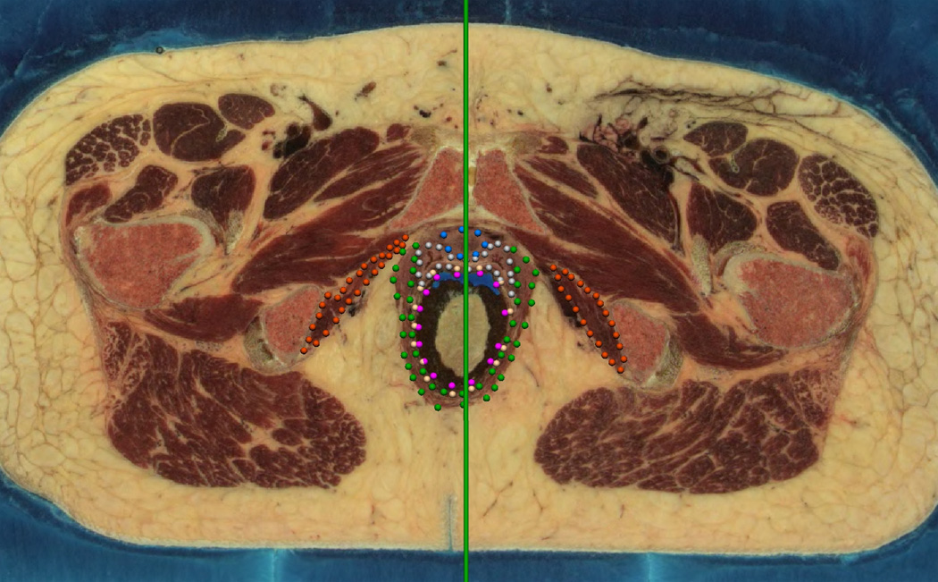
The images in the coronal and sagittal views allowed the initial digitization data clouds to be reviewed by simultaneously viewing the data in two planes as shown in Figure 1. One view remained in the original transverse (axial) (Figure 1(a)) orientation. In this view the green vertical line shows the location of the alternative sagittal view which is shown in Figure 1(b) along with the digitized ‘transverse’ points corresponding to this sagittal view. In this second view, the gold spheres indicate the points which correspond to the transverse image shown in panel (a).

Fig. 1. Dual Digitizing Windows.

A transverse (axial) view used for digitizing the Visible Woman is seen in (a) whilst (b) shows a sagittal plane used to review each of the digitized points. The green vertical bar in (a) indicates the position of the corresponding sagittal image plane shown in (b). The gold points in (b) represent those data points on the transverse slice corresponding to the transverse slice shown in (a).

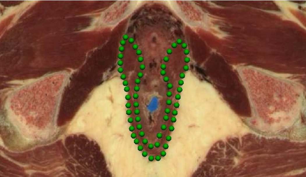
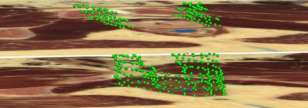
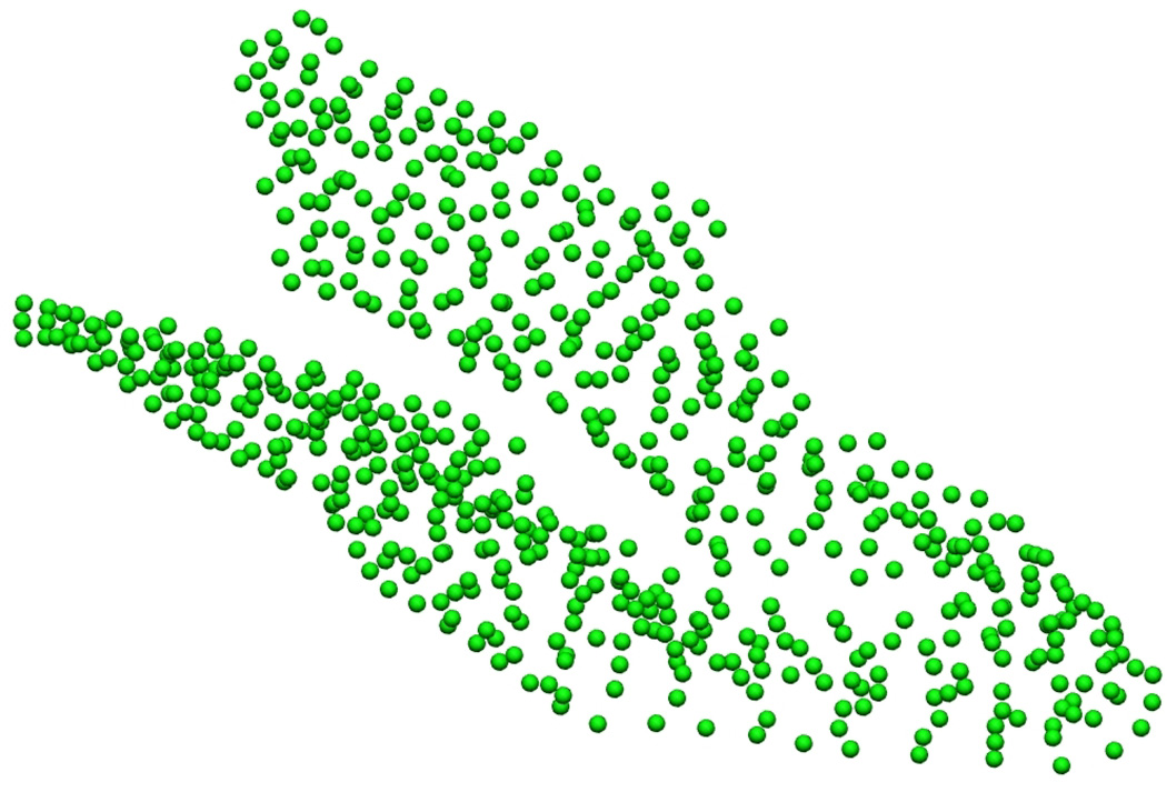
Figure 2(a) shows a tranverse (axial) slice from the Visible Man data set at a level just below the prostate and seminal vesicles. It depicts the digitized border of the puborectalis muscle which is seen outlined by green data points. Following digitization, the traced images were aligned and stacked in three-dimensional space, thus combining the data points from all the images to provide surface data for each of the structures in the pelvic floor (see Figure 2(b) and Figure 2(c)).

Fig. 2. Puborectalis Digitization Process.

Digitized Visible Man data set showing (a) an image slice outlining the puborectalis (PR) muscle in green, (b) the stack of images aligned in three-dimensional space and (c) the resulting data cloud.

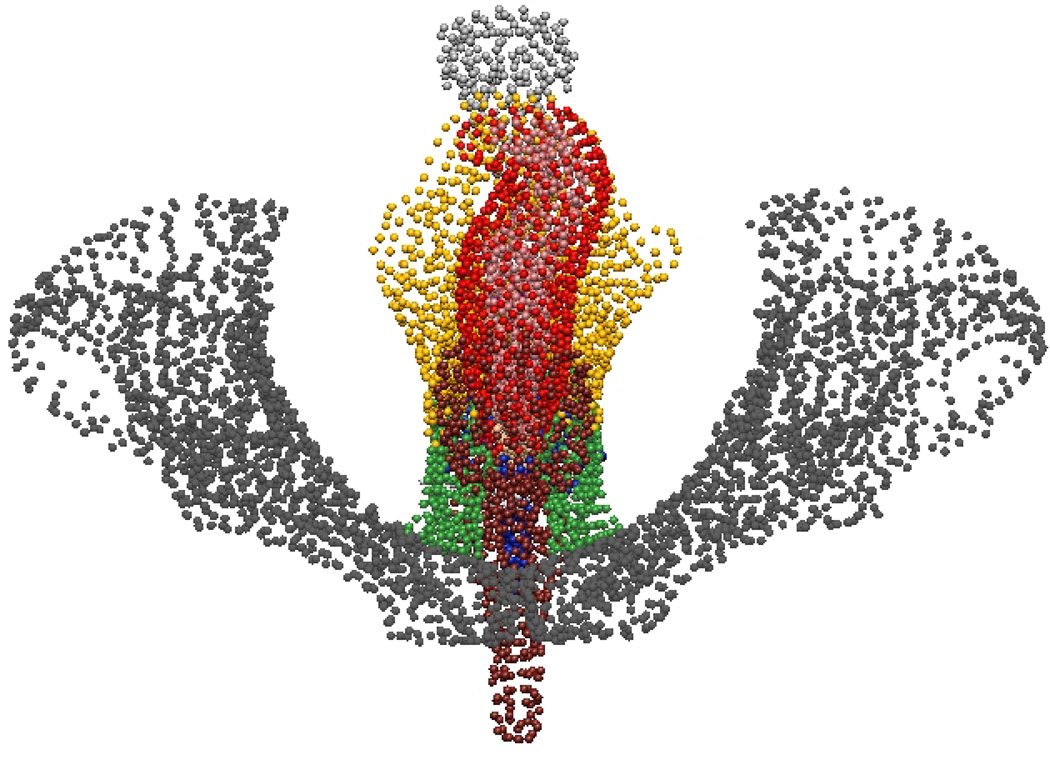
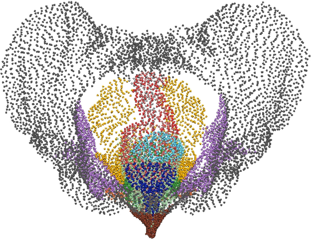
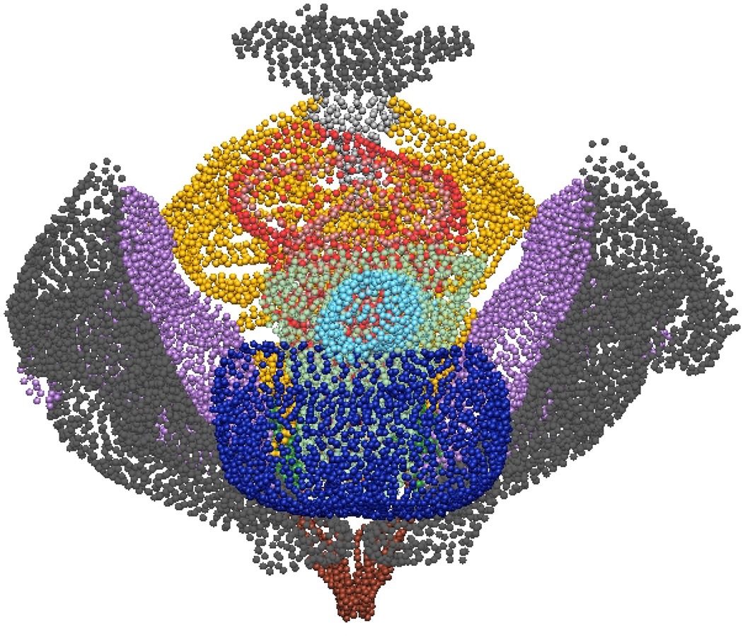
A total of 7, 605 data points were digitized for the VM mesh, compared with 12, 991 data points for the VW mesh and 19, 678 data points for MRI mesh. Figure 3 shows the finalized data clouds used to create the initial linear surface and volume meshes.

Fig. 3. Complete Mesh Data Clouds.

Traced slices are combined to give a ‘data cloud’ of anatomical information in three-dimensional space. Shown in (a) are data points for the 10 digitized components from the Visible Man while (b) and (c) show the 14 and 13 structures respectively, digitized from Visible Woman and MRI data sets.

C. Mesh Creation

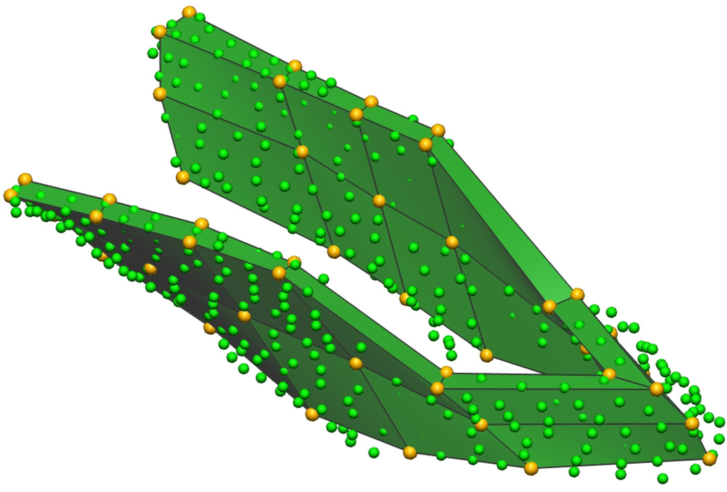
Following the 3D digitization process, the traced data sets were used to form geometric meshes which can be used as computational meshes in the finite element method using similar methods as those described in [1], [3]. Initial volume meshes were constructed for each mesh by selecting appropriate data points to be nodal points. Trilinear basis functions were then used to interpolate the initial finite elements (as seen in Figure 4(a)).

Fig. 4. Puborectalis Mesh.

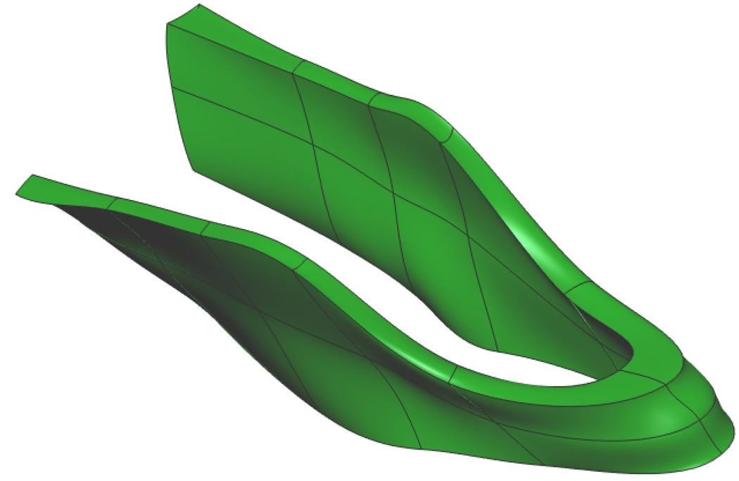
Initial mesh of the male puborectalis muscle (a) with trilinear finite elements. Nodal points are shown in gold, and the digitized data points in green. Fitted male puborectalis muscle (b) with cubic Hermite elements. The sharp edges seen on the outer edges of the mesh correspond to positions where the muscle attaches to the pubis (anteriorly – seen at the top left of the image), the levator ani (superiorly) and external anal sphincter (inferiorly).

An iterative fitting procedure with tri-cubic Hermite basis functions was used to minimize the orthogonal distances between the traced data points and their projected position on each element surface. Each traced data point was projected orthogonally onto the closest face of the mesh with the smallest distance between the two calculated using the Newton-Rhapson Method. This produced a smooth C¹ continuous surface for each pelvic floor component (shown in Figure 4(b)). The fitting method can be expressed mathematically as:

$$\text{minimise}\mathrm{F}(\mathrm{u})=\sum _{\mathrm{d}=1}^{\mathrm{D}}{\mathrm{w}}_{\mathrm{d}}{\Vert \mathit{u}({\xi }_{\mathrm{d}})-{\mathit{u}}_{\mathrm{d}}\Vert }^2$$ (1)

where d is one data point from a total of D digitized data points, having a weighting w_d and position u_d and u(ξ_d) is the location of the orthogonal projection of that data point onto the corresponding surface of the generic mesh.

D. Sobolev Smoothing

To cope with errors introduced as part of the digitisation process and account for sparse and non-uniformly distributed data a Sobolev smoothness constraint was introduced [25], [1]. This provided a penalty against excessive curvature and/or changes in volume during the fitting procedure thus producing a more realistic looking mesh. The smoothing constraint is given in Equation 2 and is added to the original objective function in Equation 1.

$$\underset{\mathrm{\Omega }}{\int }g(u(\mathit{\xi }))d\mathit{\xi }=\underset{\mathrm{\Omega }}{\int }\alpha ({\Vert \frac{\partial u}{\partial {\xi }_1}\Vert }_2+{\Vert \frac{\partial u}{\partial {\xi }_2}\Vert }_2)+\beta ({\Vert \frac{{\partial }^{2}u}{\partial {{\xi }_1}^2}\Vert }_2+2{\Vert \frac{{\partial }^{2}u}{\partial {\xi }_1\partial {\xi }_2}\Vert }_2+{\Vert \frac{{\partial }^{2}u}{\partial {{\xi }_2}^2}\Vert }_2)d\mathit{\xi }$$ (2)

where Ω is the entire solution domain and the weighting values α and β penalize changes in volume and excessive curvature respectively. Altering these weights alters the Sobolev value.

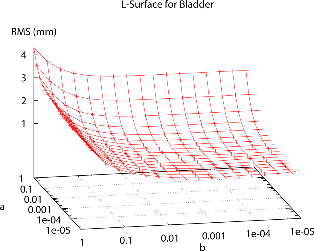
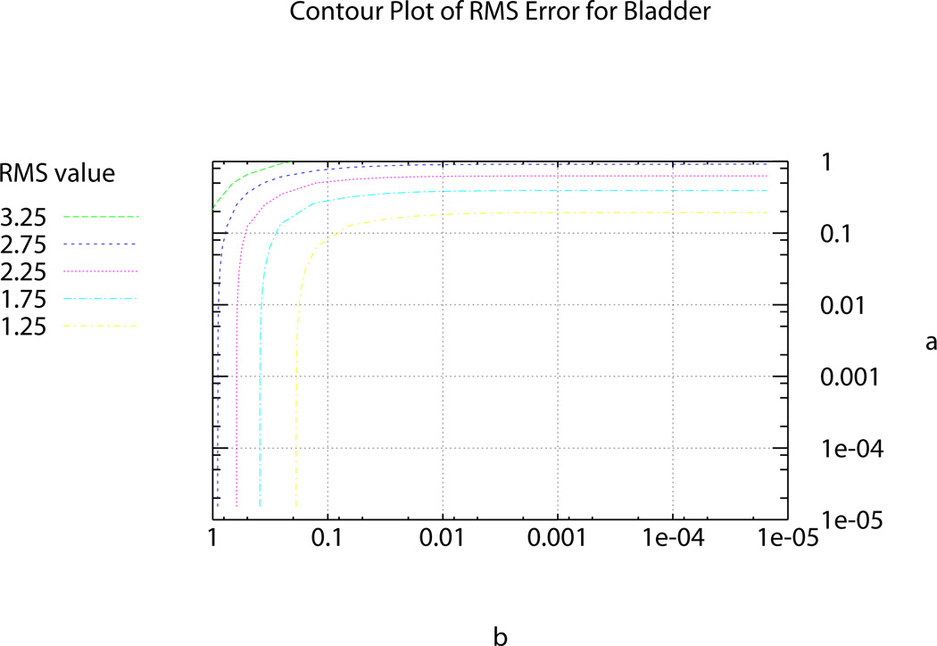
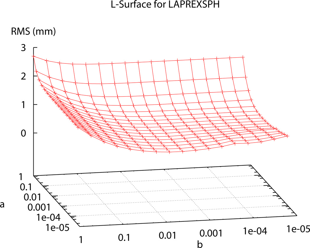
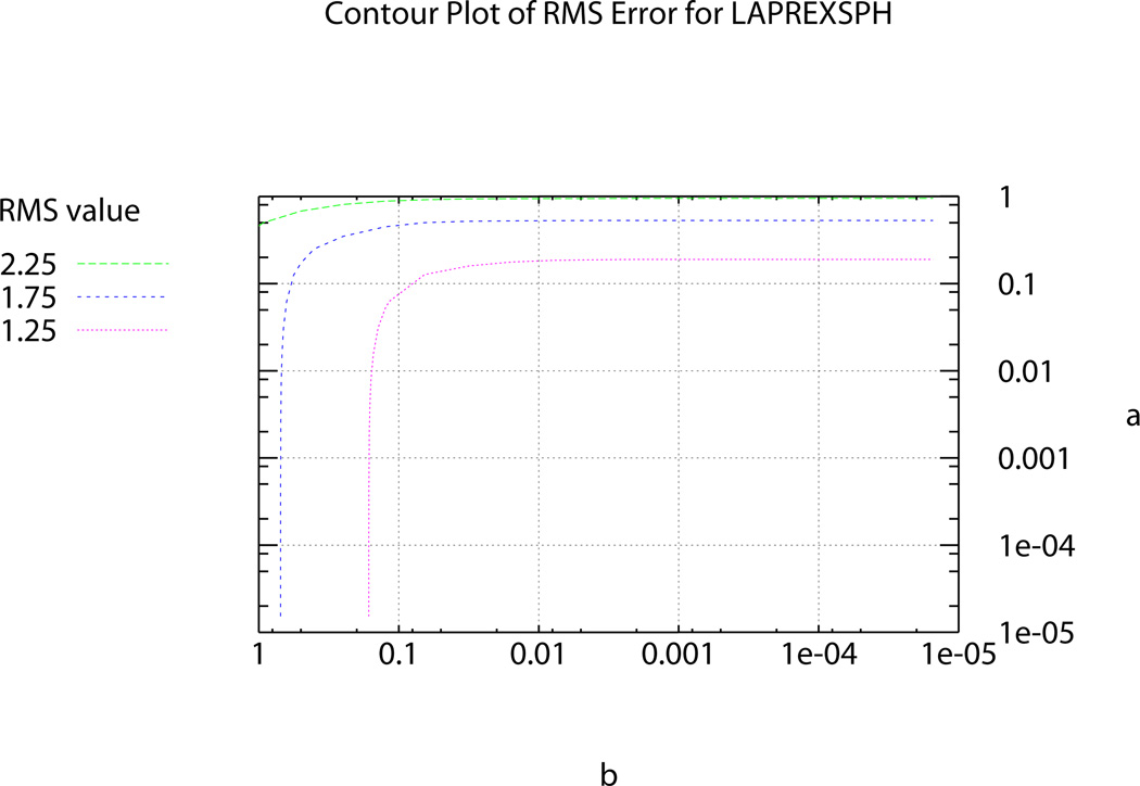
In the past, Sobolev values have been chosen using heuristic methods until a visually pleasing mesh, with acceptable RMS error, was obtained [1]. In order to determine the ‘ideal’ α and β Sobolev weights for use in the fitting procedures, two ‘L’-curve plots were produced; one for the two-dimensional surface meshes – represented by the bladder (see Figure 5) – and one for the levator ani, puborectalis and external anal sphincter muscle group (presented as LAPREXSPH) – representing the three-dimensional volume meshes (see Figure 6). Using the ‘L’-curves an ‘optimal’ point or region can be identified (i.e., a point where reducing α and/or β does not provide any significant gains in reducing RMS error) [7], [2]. To produce the plots each weighting value was independently varied from 0.5 to 1 × 10⁻⁵ and the resulting RMS value for each weighting combination was calculated and plotted on the curve following the fitting of each of the representative meshes.

Fig. 5. Sobolev Weights Plot for the Bladder.

Plot (a) shows the range of of α and β values and the corresponding RMS values produced under different weighting combinations for the bladder. (b) shows a top view of the contours to better show the RMS values at each point.

Fig. 6. Sobolev Weights Plot for the Levator Ani, Puborectalis and External Anal Sphincter Muscles.

Plot showing range of of α and β values and the corresponding RMS values produced under different weighting combinations for the LAPREXSPH muscle group.

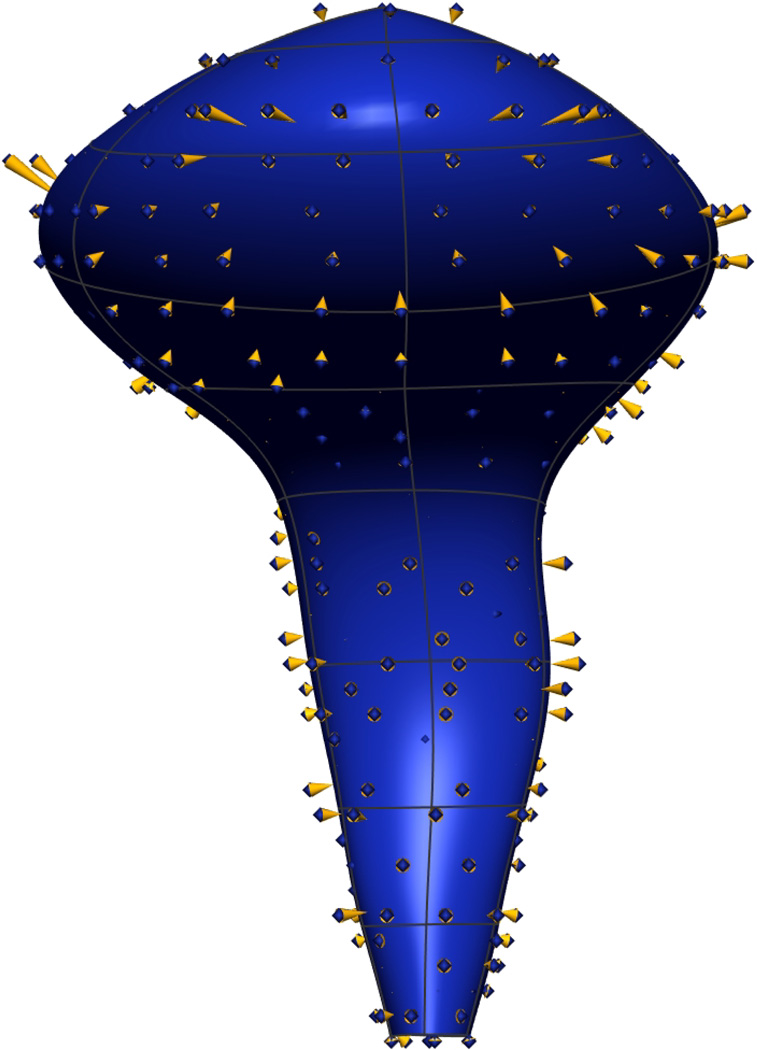
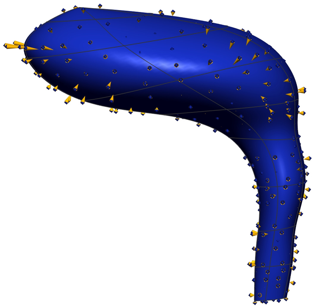
The α and β values chosen to be used in the fitting process for the bladder and the LAPREXSPH muscle group (α=0.0625, β=0.125 and α=0.125, β=0.125 respectively) occur at the ‘optimal’ point, corresponding to the point of highest curvature on the ‘L’-curve. Using these ‘ideal’ weights gives the final, realistic shape of the bladder and the levator ani, puborectalis and external anal sphincter muscles shown in Figure 7.

Fig. 7. Ideal Weighting Choices for the Bladder and LAPREXSPH Muscle Group.

Final fitted meshes of from the VW mesh with error projections (gold cones) between the fitted surface and data points. Shown are anterior (a) and lateral left (b) views of the bladder with ‘ideal’ Sobolev weighting choice (α = 0.0625, β = 0.125) giving an RMS error value of 1.24 mm. Also shown are the anterior (c) and lateral left (d) views of the LAPREXSPH muscle group with ‘ideal’ Sobolev weighting choice (α = 0.125, β = 0.125) giving an RMS error value of 1.34 mm. In both cases, weights were taken from the point of highest curvature on Figure 5(a) and Figure 6(a).

Producing a mesh with a minimum RMS error does not always create the most desirable mesh. This is primarily because there is a degree of human error associated with the manual placement of data points. Matching the mesh surface exactly to these data points may result in sharp or wrinkly edges which do not generally occur in nature. Therefore, a balance between a relatively low RMS mesh error and an over-smoothed surface must be determined by the ‘L’-curve.

The entire digitization and mesh fitting process for the VW mesh took approximately 7 days: 2 days for the initial digitization in the transverse (axial) plane, a further 3 days for the review and correction of data point placement in the alternative views and a further 2 days to fit the initial meshes to the data. This process was shorter for the MRI mesh as there were less images to digitise and review and the VW mesh was used as a guide.

E. Mesh Fitting Results

Using the ‘ideal’ Sobolev values calculated in Section II-D the remaining pelvic floor structures were fitted to the data clouds to produce the final mesh components. Producing plots such as Figure 5 and Figure 6 is a time consuming process and so was only followed for two meshes (one surface and one volume). The α and β weights selected for this study were ‘ideal’ for producing realistic looking bladder and LAPREXSPH muscle meshes for which they were specifically calculated, but were not necessarily ‘ideal’ for all of the other surface and volume meshes produced as the exact degree of smoothing required will depend on the shape of each structure and the consistency and accuracy of the data point placement. A visual check was used on all the fitting procedures which guided the use of these weights for all other meshes. In the future, it may be possible to streamline this process by using an optimization algorithm to determine the best parameters for each structure.

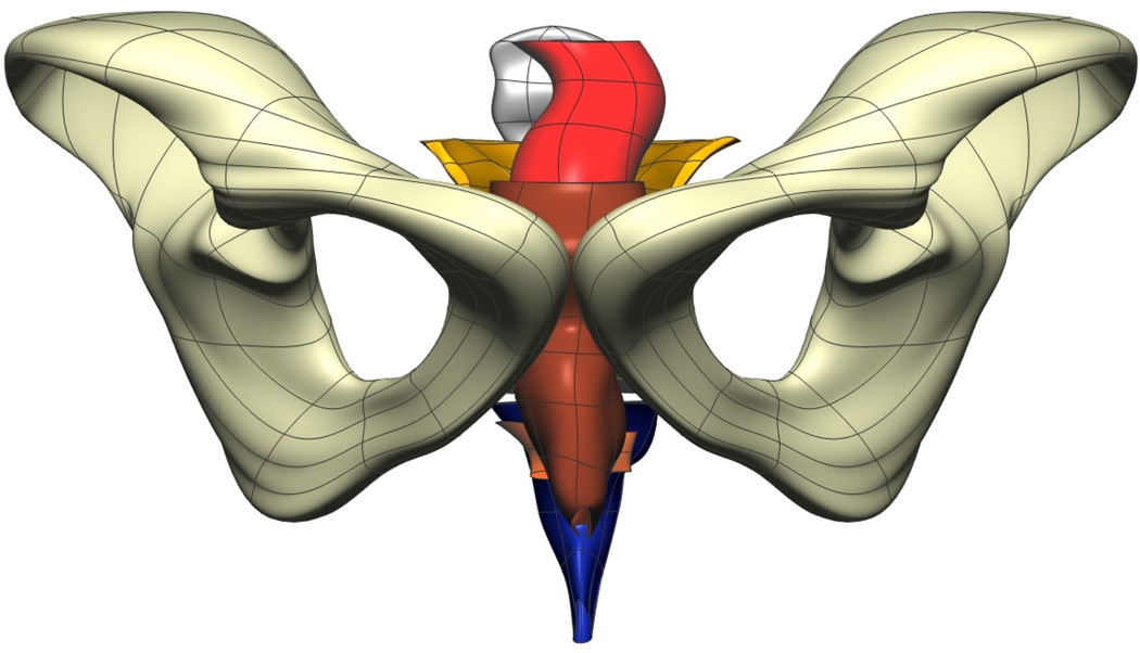
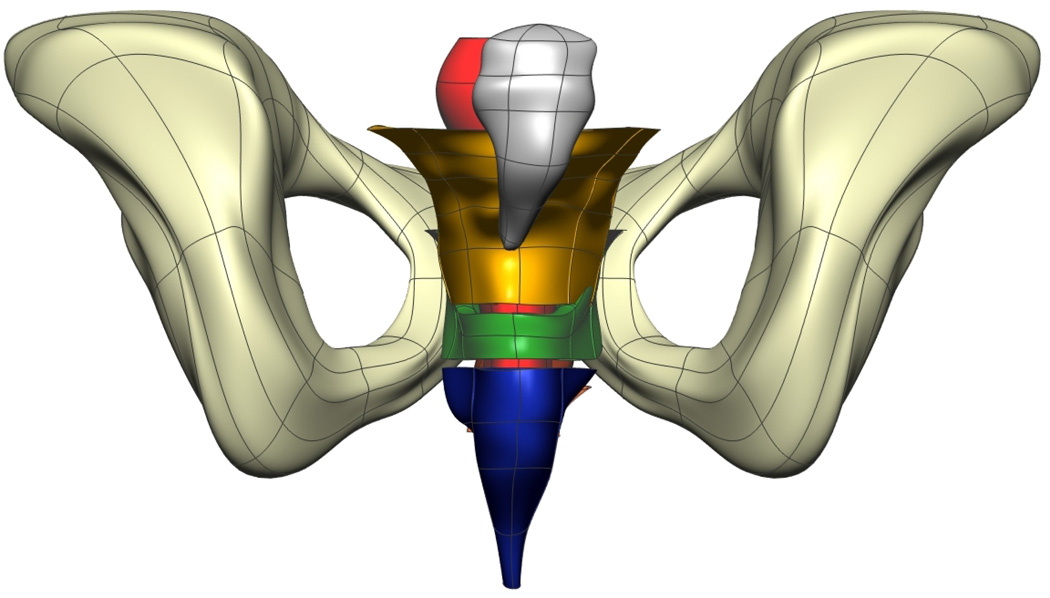
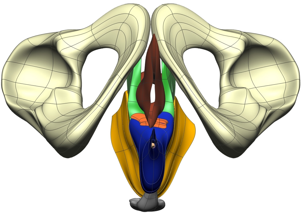
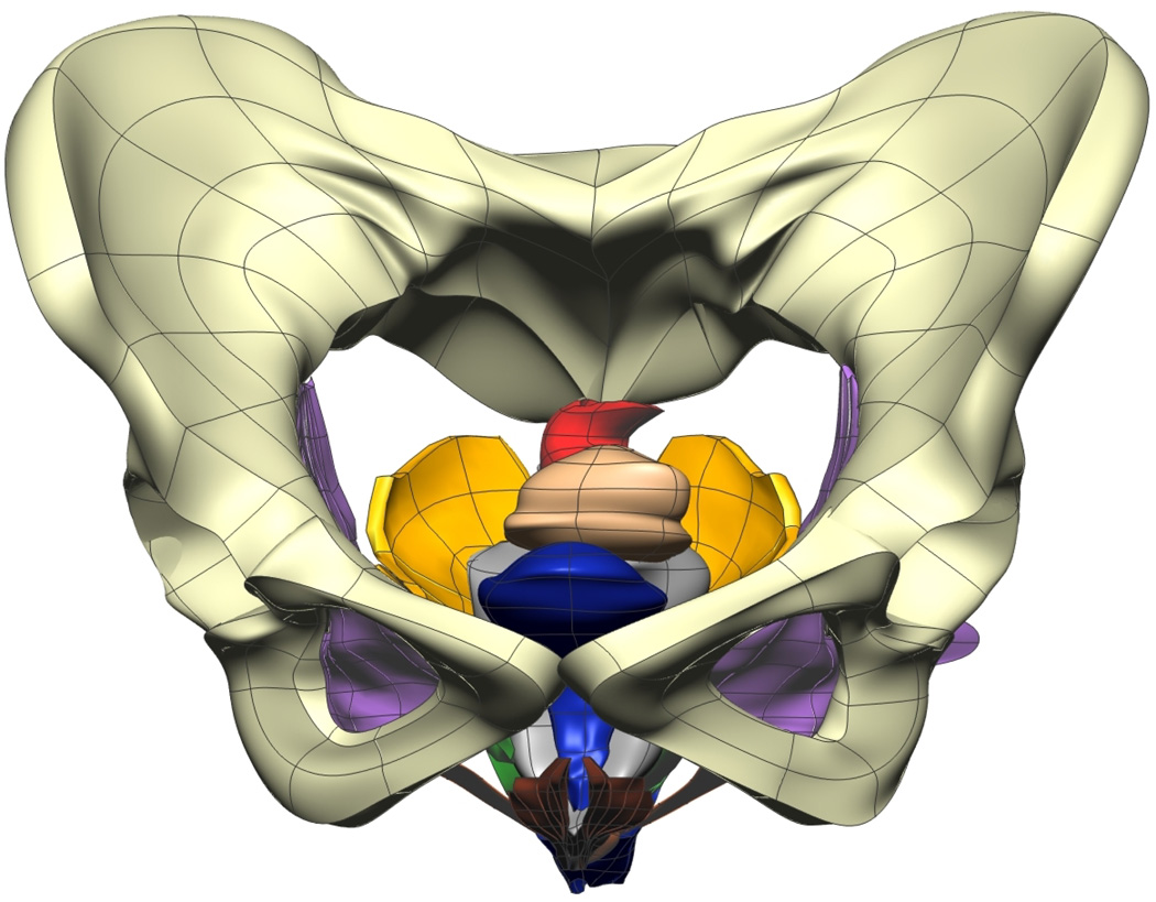
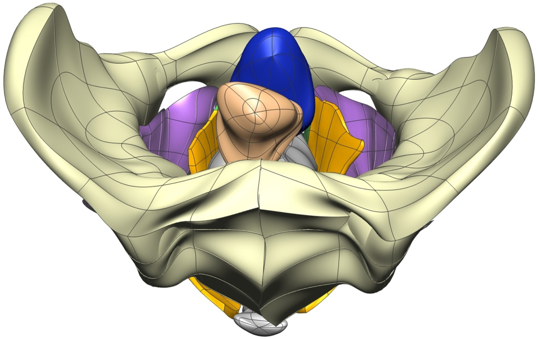
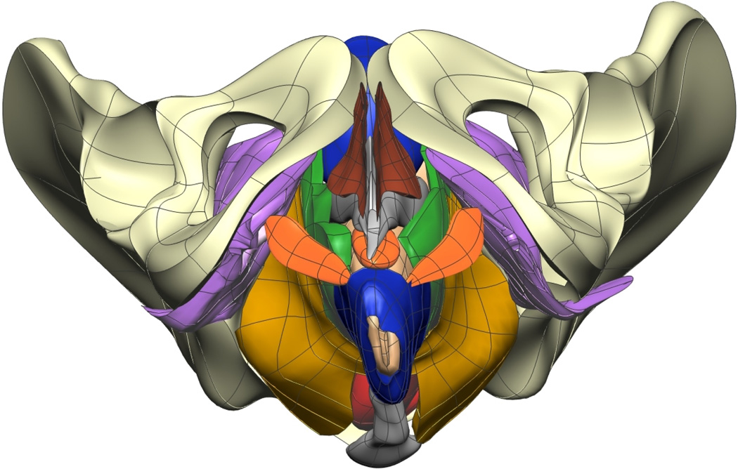
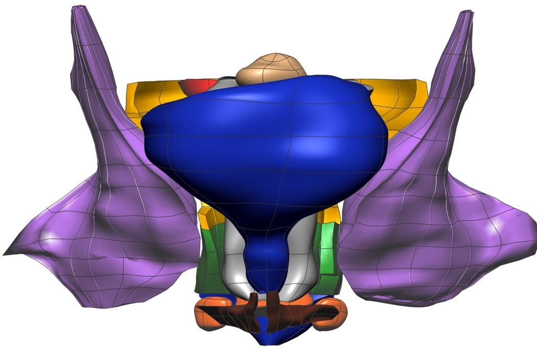
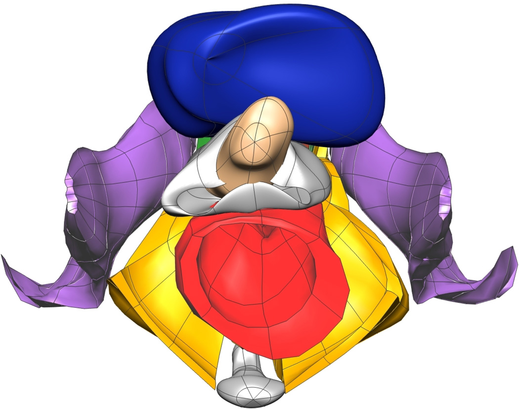
The individual mesh geometries were then assembled together to form the complete pelvic meshes for the Visible Man, Visible Woman shown in Figure 8 and Figure 9. Results for each of the VM pelvic floor structures gave an average RMS error less than 0.8 mm, and the VW meshes gave average RMS errors less than 1.15 mm (see Table II and Table III).

Fig. 8. Visible Man Final Mesh Views.

Final fitted meshes from the Visible Man data set. Shown are (a) anterior, (b) posterior, (c) cephalad and (d) caudad views showing the 10 components – PR (green), LA (gold), EAS (blue), IAS (beige), rectum (red), lumen (purple), TP (orange), pubis (white), coccyx (silver) and UPBS group (brown).

Fig. 9. Visible Woman Final Mesh Views.

Final fitted meshes from the Visible Woman data set. Shown are (a) anterior, (b) posterior, (c) cephalad and (d) caudad views showing 13 of the 14 components – PR (green), LA (gold), EAS (blue), IAS (beige), rectum (red), TP (orange), PB (orange), coccyx (silver), uterus (beige), vagina (silver), OI (purple) and bulbospongiosus (brown). For clarity the lumen has not been included.

TABLE II. Fitting Results for the VM Mesh.

Summary of the VM fitting results obtained by fitting piece-wise bi- and tri-cubic Hermite surfaces to digitized cyrosection photographs from the VM. The RMS errors (mm) are between the digitized data points and their orthogonal projections onto the fitted surfaces.

Component	No. Data Pts	No. Nodes	No. Elem.	RMS Error (mm)
LA	918	59	20	0.94
PR	640	66	20	0.57
Rectum	696	48	42	0.57
Lumen	565	60	54	0.40
IAS	207	42	18	0.89
EAS	708	54	24	1.02
Pubis	1168	96	84	1.27
Coccyx	219	38	42	0.53
TP	89	18	12	1.01
UPBS	567	42	36	0.72

TABLE III. Fitting Results for the VW Mesh.

Summary of the VW fitting results obtained by fitting piece-wise bi- and tricubic Hermite surfaces to digitized cyrosection photographs of the VW. The RMS errors are calculated as the difference between the digitized data points and their orthogonal projections onto the fitted surfaces.

Component	No. Data Pts	No. Nodes	No. Elem.	RMS Error (mm)
LAPREXSPH	2436	396	167	1.34
LA	1083	166	65	–
PR	704	96	45	–
EAS	649	70	57	–
LURECINSPH	1639	180	78	1.09
Lumen	785	*	*	–
Rectum	439	48	62	–
IAS	415	42	16	–
Pubis	4747	308	108	2.0
Coccyx	88	36	30	0.65
TP	123	32	24	1.59
PB	115	24	18	0.66
Bladder	364	45	40	1.24
Uterus	244	48	42	0.89
Vagina	881	72	64	1.19
Bulbospongiosus	567	32	24	1.01
Obturator Internus	1834	288	132	0.89

^*In order to create volume meshes for the rectum and internal anal sphincter muscles, the lumen data was used to form the inner surfaces, therefore, no nodes or elements are associated with the lumen surface.

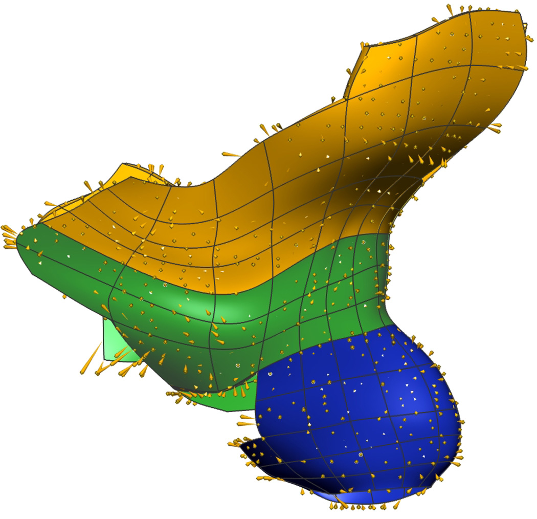
Thirteen volume and surface meshes from the Visible Woman mesh were independently fitted to the data obtained from the subject-specific images and the number of nodes and elements were altered as necessary in order to obtain the best fit to the subject data. Views of the final fitted MRI mesh is shown in Figure 10 and in Figure 11 overlaid with MRI image planes from which the mesh was constructed. Fitting results are shown in Table IV. The average RMS error for the subject-specific mesh was less than 0.75 mm.

Fig. 10. Subject-specific MRI Mesh Views.

Final fitted meshes from the MRI data set. Shown are (a) anterior, (b) posterior, (c) cephalad and (d) caudad views showing 12 of the 13 components – PR (green), LA (gold), EAS (blue), IAS (beige), rectum (red), TP (orange), PB (orange), coccyx (silver), uterus (beige), vagina (silver), OI (purple) and bulbospongiosus (brown). For clarity the lumen has not been included.

Fig. 11. Subject-specific MRI Final Mesh.

Lateral left view of the combined meshes which form the subject-specific MRI mesh. The mesh is seen in relation to the original three-dimensional MR images and texture block.

TABLE IV. Fitting Results for the Subject-Specific MRI Mesh.

Summary of the subject-specific MRI fitting results obtained by fitting piece-wise bi- and tricubic Hermite surfaces to digitized MRI slices of a particular female subject. The RMS errors are calculated as the difference between digitized data points and their orthogonal projections onto the fitted surfaces.

Component	No. Data Pts	No. Nodes	No. Elem.	RMS Error (mm)
LAPREXSPH	4335	314	128	1.03
LA	2830	169	58	–
PR	875	120	39	–
EAS	630	78	28	–
LURECINSPH	1831	114	54	0.78
Lumen	691	*	*	–
Rectum	981	84	36	–
IAS	159	42	18	–
Coccyx	217	38	42	0.45
TP	157	28	32	0.94
PB	107	24	18	0.48
Bladder	1477	46	45	0.68
Uterus	375	31	30	0.52
Vagina	1250	64	56	0.84
Bulbospongiosus	388	74	23	0.66
Obturator Internus	3570	288	132	1.03

^*In order to create volume meshes for the rectum and internal anal sphincter muscles, the lumen data was used to form the inner surfaces, therefore, no nodes or elements are associated with the lumen surface.

Key muscles within the pelvic floor which are interconnected (i.e., the levator ani, puborectalis, external anal sphincter and also the rectum and internal anal sphincter) were represented by combining the individual components together in the VW and MRI meshes. The mesh LAPREXSPH represents the levator ani, puborectalis and external anal sphincter group and the LURECINSPH mesh represents the rectum and internal anal sphincter with the lumen running through the middle.

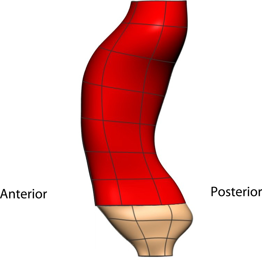
The main flaw in the VM model is the rectum and anal canal appear to be compressed and do not lie in the normal orientation that is expected in live subjects. Figure 12(a) shows the angle between the rectum (red) and anal canal (beige) in the VM was relatively flat and was thought to have been caused by the post-mortem perineal pressure on the posterior surface of the cadaver caused by the body of the cadaver conforming to the container before it was frozen and imaged. This distortion does not allow an accurate representation of the male pelvic floor region to be constructed from the data as it does not depict the known angle between the distal rectum and proximal anal canal. In contrast, the VW mesh (shown in Figure 12(b)) depicts the expected anorectal angle more accurately. The distension of the VW anal canal was probably due to post mortem changes with anal packing during the embalming process.

Fig. 12. Visible Human Rectum Comparison.

Lateral view of the VM (a) and VW (b) rectum and anal canal. The angle between the rectum (red) and anal canal (pink) in the VM was relatively flat due to post-mortem perineal pressure and does not depict the known angle between the distal rectum and proximal anal canal which was present in the VW.

III. Discussion

Three computational, anatomically realistic meshes of the pelvic floor and anal canal region have been developed from different data sets. Two cadaver-based meshes were produced using the Visible Human Project cryosection data sets and a third mesh was produced based on MR image data. The Visible Man mesh included 10 different pelvic structures; the rectum, the puborectalis muscle, the levator ani muscle group, the internal and external anal sphincters, the transverse perineae muscles, the pubis and coccyx bones, and the urethra/prostate and bulbospongiosus group. The Visible Woman mesh contained 14 individual structures namely; the rectum, vagina, uterus and bladder (including urethra), the puborectalis, levator ani muscle group, internal anal sphincter, external anal sphincter, transverse perineae muscles, the obturator internus muscles, the bulbospongiosus muscle, the pelvis and coccyx bones and the perineal body. Missing from the meshes are the locations of the major blood vessels and nerves within the pelvic region. The inclusion of these components would be highly beneficial for future functional simulations and for surgical planning, however, due to their size the nerves and blood vessels could not be clearly visualized on the images. All but the larger blood vessels were collapsed in the VH images, however, with the use of intravenous constrast it is possible that they could be visualized via MRI.

RMS error is relative to the size of the structure being meshed. An average RMS error of under 0.8 mm was achieved in the VM and MRI meshes and an average RMS error under 1.15 mm was achieved for the VW meshes. These are low compared to previous modeling work [1], [6] which achieved RMS errors of under 2 mm and under 5 mm respectively. Ultimately, the RMS error was a check of how close the data points lie to the surface of the mesh and therefore basing the fit entirely on this factor may be misleading. The subjective appearance of the mesh is also important and often a more uniform appearance, which comes at the price of a higher RMS value, may be preferred.

New Sobolev smoothing weights were calculated for the use in both the surface and volume mesh fitting procedures. ‘L’-curves were produced for the calculation, and the ‘ideal’ weights were taken at the point of highest curvature on each graph. The use of these weights (α = 0.0625, β = 0.125 for surface meshes and α = 0.125, β = 0.125 for volume meshes) produced geometries which accurately represented the pelvic anatomy.

As each new mesh was constructed, the time taken to construct the next mesh was significantly reduced as prior knowledge and information gained could be used for the following meshes (e.g., the initial linear meshes from the VW were used as a starting point for creating the linear subject-specific meshes and required only minor adjustments to follow the subject data as closely as possible and become useful as initial meshes for the MRI mesh). Therefore, despite the MR images being the poorest quality, the MRI mesh was the quickest to construct, being the last, and was aided greatly by similar reference points on the VW images and mesh. Thus, the creation of additional MRI meshes should be relatively straight forward. Once we have a larger number of geometric meshes from different subjects, it will be possible to assess whether it is possible to rapidly adapt existing meshes to match other datasets (e.g., by non-linear scaling in different regions [14]).

It remains undetermined whether the VW subject was nulliparous or whether she had ever been pregnant. The live patient scanned in our MRI study was nulliparous and had never been pregnant. Efforts were made to try and find out the history of the VW but these were unsuccessful. If the VW had carried and/or given birth to one or more babies then this may have affected her pelvic region, especially the muscles situated around or near the vagina which are those most pertinent to this study [8]. It is important that further enquiries be carried out to resolve this issue.

Although the VHP data sets were of a very high resolution the subjects had undergone some significant postmortem changes [22] before they were imaged. In the VM this was most clearly seen in the distortion of the anal canal presumably due to postmortem pressure on the perineum. This led to the cadaveric male mesh having an abnormally oriented anal canal without the accepted posterior angulation at the ano-rectal junction [11]. These postmortem abnormalities can be overcome by comparing the mesh with a mesh based on a live subject.

Previous studies have shown that racial differences can play a part in determining the morphology of pelvic structures [9] and there are undoubtably differences due to age and anthropometry, thus, with only 3 meshes we remain with only a limited view of ‘normal’ pelvic anatomy within a population and additional meshes are needed in order to adequately classify any suspected abnormalities in the pelvic floor and also to properly assess which customization methods may be best suited to adapt existing meshes to match different subject data.

We envision that with further devlopment these meshes may, in the future, allow clinicians, patients and students alike to improve their understanding of this complicated area, and to better understand the relationship between different components within this region. It may also be feasible for these meshes to be used to provide a simple simulation environment for the virtual planning of corrective surgery. The meshes have been constructed in a manner which allows them to be used in the future for functional finite element simulations (as opposed to being only being able to be used visually). The MRI mesh presented here has, in fact, been used in a separate study to examine the mechanics of normal function of the levator ani muscle group during a ‘bear down’ or abdominal squeeze maneuver [16]).

IV. Conclusions

The overall objective of this research was to create accurate, anatomically representative three-dimensional meshes of both the male and female pelvic floor regions in order to improve the understanding of the pelvic floor and anal canal.

This study has shown that it was possible to create a realistic computational mesh based on a high resolution cadaver data set. These meshes were also used to assist in producing a subject-specific mesh based on MRI data of lower resolution. Producing a subject-specific mesh was a significant achievement in this research as it provides a validation of the accuracy of the cadaver-based meshes, and provides a means to overcome the limitations of postmortem changes in tissue orientation. This ability to produce realistic subject-specific computational meshes is a major step towards developing patient-specific meshes that can guide the management of individual patients with defecatory disorders.

References

- 1.Bradley CP, Pullan AJ, Hunter PJ. Geometric modeling of the human torso using cubic Hermite elements. Ann. Biomed. Eng. 1997;25:96–111. doi: 10.1007/BF02738542. [DOI] [PubMed] [Google Scholar]
- 2.Cheng LK, Bodley JM, Pullan AJ. Comparison of potential and activation based formulations for the inverse problem of electrocardiology. IEEE Trans. Biomed. Eng. 2003 Jan;50:11–22. doi: 10.1109/TBME.2002.807326. [DOI] [PubMed] [Google Scholar]
- 3.Cheng LK, Sands GB, French RL, Withy SJ, Wong SP, Legget ME, Smith WM, Pullan AJ. Rapid construction of a patient-specific torso model from 3D ultrasound for non-invasive imaging of cardiac electrophysiology. Med Biol Eng Comput. 2005;43:325–330. doi: 10.1007/BF02345808. [DOI] [PubMed] [Google Scholar]
- 4.d’Aulignac D, Martins JAC, Pires EB, Mascarenhas T, Jorge RMN. A shell finite element model of the pelvic floor muscles. Comput. Methods Biomech. Biomed. Engin. 2005;8:339–347. doi: 10.1080/10255840500405378. [DOI] [PubMed] [Google Scholar]
- 5.Drossman DA, Li Z, Andruzzi E. U.S. householder survey of functional gastrointestinal disorders: Prevalence, sociodemography, and health impact. Dig. Dis. Sci. 1993;38:1569–1580. doi: 10.1007/BF01303162. [DOI] [PubMed] [Google Scholar]
- 6.Fernandez JW, Mithraratne P, Thrupp SF, Tawhai MH, Hunter PJ. Anatomically based geometric modelling of the musculo-skeletal system and other organs. Biomech. Model. Mechnobiol. 2004 Mar;2:139–155. doi: 10.1007/s10237-003-0036-1. [DOI] [PubMed] [Google Scholar]
- 7.Hansen PC, O’Leary DP. The use of the L-curve in the regularisation of discrete ill-posed problems. SIAM J. Sci. Comput. 1993 Nov;14:1487–1503. [Google Scholar]
- 8.Hoyte L, Damaser MS. Magnetic resonance-based female pelvic anatomy as relevant for maternal childbirth injury simulations. Ann. N. Y. Acad. Sci. 2007 Apr;1101:361–376. doi: 10.1196/annals.1389.018. [DOI] [PubMed] [Google Scholar]
- 9.Hoyte L, Thomas J, Foster RT, Shott S, Jakab M, Weidner AC. Racial differences in pelvic morphology among asymptomatic nulliparous women as seen on three-dimensional magnetic resonance images. Am. J. Obstet. Gynecol. 2005 Dec;193:2035–2040. doi: 10.1016/j.ajog.2005.06.060. [DOI] [PubMed] [Google Scholar]
- 10.Janda S, van der Helm FCT, de Blok SB. Measuring morphological parameters of the pelvic floor for finite element modelling purposes. J Biomech. 2003;36:749–757. doi: 10.1016/s0021-9290(03)00008-3. [DOI] [PubMed] [Google Scholar]
- 11.Last RJ. Anatomy, Regional and Applied. Churchill Livingstone: Medical Division of Longman Group Limited; 1984. [Google Scholar]
- 12.Locke GR, Pemberton JH, Phillips SF. Aga technical review on constipation. Gastroenterology. 2000;119:1766–1778. doi: 10.1053/gast.2000.20392. [DOI] [PubMed] [Google Scholar]
- 13.Macmillan AK, Merrie AEH, Marshall RJ, Parry BR. The prevalence of fecal incontinence in community-dwelling adults: A systematic review of the literature. Dis Colon Rectum. 2004;47:1341–1349. doi: 10.1007/s10350-004-0593-0. [DOI] [PubMed] [Google Scholar]
- 14.Nash MP, Bradley CP, Cheng LK, Pullan AJ, Paterson DJ. An in-vivo experimental-computational framework for validating ECG inverse methods. Intl. J. Bioelectromagnetism. 2000 Sep;2 [Google Scholar]
- 15.Nelson R, Norton N, Cautley E, Furner S. Community based prevalence of anal incontinence. JAMA. 1995;274:559–561. [PubMed] [Google Scholar]
- 16.Noakes KF, Pullan AJ, Bissett IP, Cheng LK. Subject specific finite elasticity simulations of the pelvic floor. J. Biomech. 2008;41(14):3060–3065. doi: 10.1016/j.jbiomech.2008.06.037. [DOI] [PMC free article] [PubMed] [Google Scholar]
- 17.Parente MP, Jorge RM, Mascarenhas T, Fernandes AA, Martins JA. Deformation of the pelvic floor muscles during a vaginal delivery. Int. Urogynecol. J. Pelvic Floor Dysfunct. 2007 doi: 10.1007/s00192-007-0388-7. [DOI] [PubMed] [Google Scholar]
- 18.Seymour SD. Fecal incontinence. Internet. 2006 Jun; http://www.emedicine.com/med/topic3326.htm.
- 19.Siproudhis L, Pigot F, Godeberge P, Damon H, Soudan D, Bigard MA. Defecation disorders: A french population survey. Dis Colon Rectum. 2006;49:219–227. doi: 10.1007/s10350-005-0249-8. [DOI] [PubMed] [Google Scholar]
- 20.Smith CA, Witherow RON. The assessment of female pelvic floor dysfunction. BJU International. 2000;85:579–587. doi: 10.1046/j.1464-410x.2000.00474.x. [DOI] [PubMed] [Google Scholar]
- 21.Spitzer V, Ackerman MJ, Scherzinger AL, Whitlock D. The visible human male: A technical report. J. Am. Med. Inform. Assoc. 1996 Mar;3:118–130. doi: 10.1136/jamia.1996.96236280. [DOI] [PMC free article] [PubMed] [Google Scholar]
- 22.Spitzer VM, Scherzinger AL. Virtual anatomy: An anatomist’s playground. Clin. Anat. 2006;19:192–203. doi: 10.1002/ca.20330. [DOI] [PubMed] [Google Scholar]
- 23.Verhey JF, Wisser J, Warfield SK, Rexilius J, Kikinis R. Non-rigid registration of a 3D ultrasound and a MR image data set of the female pelvic floor using a biomechanical model. Biomed Eng Online. 2005;4:19. doi: 10.1186/1475-925X-4-19. [DOI] [PMC free article] [PubMed] [Google Scholar]
- 24.Woodburne RT, editor. Essentials of Human Anatomy. Oxford University Press; 1983. [Google Scholar]
- 25.Young AA, Hunter PJ, Smaill BH. Epicardial surface estimation from coronary angiograms. Comput. Vision Graphics Image Process. 1989;47:111–127. [Google Scholar]