Mathematical Modeling and Data Analysis of NMR Experiments using Hyperpolarized ¹³C Metabolites

Abstract

Rapid-dissolution dynamic nuclear polarization (DNP) has made significant impact in the characterization and understanding of metabolism that occurs on the sub-minute timescale in several diseases. While significant efforts have been made in developing applications, and in designing rapid-imaging radiofrequency (RF) and magnetic field gradient pulse sequences, very few groups have worked on implementing realistic mathematical/kinetic/relaxation models to fit the emergent data.

The critical aspects to consider when modeling DNP experiments depend on both nuclear magnetic resonance (NMR) and (bio)chemical kinetics. The former constraints are due to the relaxation of the NMR signal and the application of ‘read’ RF pulses, while the kinetic constraints include the total amount of each molecular species present. We describe the model-design strategy we have used to fit and interpret our DNP results. To our knowledge, this is the first report on a systematic analysis of DNP data.

Introduction

Dynamic nuclear polarization (DNP) involves saturating the magnetization of unpaired electrons in a radical-molecule (or metal ion) to lead to cross polarization of the magnetization of neighboring nuclei. Even though the theoretical description of the phenomenon in metal ions (and later on for electron spins) was made by Overhauser in 1953,1 and its experimental demonstration was in the same year by Carver and Slichter,2 experimental applications of the phenomenon did not evolve greatly over the next 50 years.

With new technological developments (high-frequency microwave sources, cryo-technology), a rapid-dissolution DNP system was created3 and commercialized (HyperSense^®, Oxford Instrument). Typically, the sample, a ¹³C-labelled compound dissolved in aqueous solution with a free radical, is cooled to ~1.4 K inside a superconducting magnet (3.35 T). The electrons of the radical are excited by microwave irradiation (~94.1 GHz) and their magnetization is transferred to the nuclei via electron-nuclear dipolar coupling. This operation takes from a few tens of minutes to several hours. At the end of the hyperpolarization process, the sample is rapidly returned to its physiological temperature (typically 37 °C) by automatically dissolving it in a buffer that is at high pressure and temperature, and the buffer-dissolved sample is shuttled via a delivery pipe (typically Teflon) to the magnet to be injected either in vitro or in vivo. The first reported signal enhancement in ¹³C NMR (urea sample) was greater than 10,000-fold.3 Over the last decade, this technique has mostly been developed for in vivo applications to detect and characterize diseases like cancer.4–10 The molecule most used to investigate metabolism has been pyruvate as it hyperpolarizes well, and rapidly enters into the tricarboxylic acid cycle (TCA cycle; or Krebs cycle) or is converted into alanine, lactate and bicarbonate. It has a reasonably long observable life-time (related to the spin-lattice relaxation T₁).11 As dissolution-DNP requires rapid recording, fast image-acquisition procedures have been developed (based on EPSI, and SPIRAL).12,13 In vivo studies have focused mostly on the ¹³C nucleus, but for completeness we note that other nuclei have been hyperpolarized, some having direct biological interest (¹⁵N,¹⁹F, ³¹P) and others being more interesting from a chemistry perspective, or as indirect biological probes (eg, ⁸⁹Y, ^107,109Ag).14–17

Huge efforts have been made to refine rapid-dissolution DNP to demonstrate its applicability in medical diagnosis. While the results are convincing, they are nevertheless preliminary. The production rate of particular metabolites is significantly different between the healthy and diseased tissues, but quantitative flux analysis is as yet naive. Most of the data fitting has been done by considering a simple one-way reaction without taking into account the enzyme concentrations or possible Michaelis-Menten-type saturation kinetics, or the possible inhibition of the reaction(s) due to the injection of a large amount of an enzyme’s substrate. From this perspective, data analyzed using a simple linear relationship between enzyme concentration/activity and the apparent reaction flux are unconvincing. During the conversion of pyruvate to lactate, some researchers have noted that increases in the lactate signal not only are due to biochemical reactions, but also to magnetization transfer between the substrate and product of the reaction.6,18

To the best of our knowledge, very few studies have used the more realistic models of enzymic reactions or investigated the use of the mathematical models of the relaxation-reaction scheme in their data analysis. One of the first studies to use a kinetic model including the Michaelis-Menten mechanism involved an animal model of prostate cancer.19 The authors showed an effect of the substrate dose on the estimates of the kinetic parameters. By combining ¹³C and ³¹P data and a “realistic” relaxation-kinetic model, Harris et al claimed that the conversion of hyperpolarized pyruvate to lactate in breast cancer cells (T47D) was limited by the rate at which the pyruvate crossed the cell membrane.8 This realization was later discussed by Witney et al20 and a recent study compared the data fitting using different models based on first-order kinetics with either two- or three-pool, uni- or bi-directional chemical reactions.21 While data from hyperpolarized substrates by themselves could be fitted by a simple 2-pool model, the inclusion of mass spectrometry data necessitated the use of a 3-pool model to achieve realistic fits to the data. Most of the developments in modeling the experiments were performed on in vitro systems. Unfortunately, none of these papers extensively explain the strategy used to design their model.

In this article, we describe the physical phenomena that must be considered when constructing a mathematical model that describes data from a rapid-dissolution DNP experiment. The strategy used to create the model and fit the experimental data is explained; it derives its concepts from the older literature used to describe ‘tracer exchange’ enzyme kinetics and its later application to magnetization transfer in NMR spectroscopy.22 To our knowledge, this is the first paper to explicitly explain in extenso the necessary constraints when modeling rapid-dissolution DNP experiments.

Hyperpolarization Considerations

The mathematical modeling of an experiment involving hyperpolarized metabolites requires account to be taken of more parameters than those in classical (bio)chemical kinetics. Some of these refinements are well described in the literature (for example,18,19,21) while others are not. In the following sections we explain the different kinetics aspects that arise as a result of the excited (hyperpolarized) state.

Spin-lattice relaxation T₁

The first key parameter that must be included in a mathematical model of the kinetics/relaxation scheme is the spin-lattice relaxation time, T₁. Indeed, after hyperpolarization, the nuclear spins relax back to a Boltzmann-distribution of states, ie, to equilibrium (at the same rate as ‘normal’ polarized spins). The magnetization at any time, t, can be expressed as a function of the initial magnetization M₀ and the relaxation time:

$$M_z(t)=M_0{e}^{-t/T_1}$$ (1)

where M_z(t) denotes the magnetization of the hyperpolarized species along the direction of the magnetic field B₀ in the NMR spectrometer magnet. According to this equation the magnetization relaxes without giving rise to an observable signal. To observe the NMR signal, the magnetization must be transferred into the x,y-plane by applying an RF pulse. This point is more broadly described in the following section.

Because the relaxation rate is dependent on both the chemical and physical environments, it is important to estimate its value for each of the species studied for all physical and biological systems. Figure 1 shows simulations of magnetization decay for a range of relaxation times; the figure reveals how critical it is to consider differences in T₁ values between different chemical species and/or media. Furthermore, in conventional NMR spectroscopy, long T₁ values are usually considered a drawback. This is because they require the use of a long recycle time (or relaxation delay) between acquisition of free induction decays (FIDs), thus ensuring so called ‘fully relaxed’ spectra that quantitatively reflect the number of spins in the sample. However, as shown in Fig. 1, for hyperpolarized spins in which the signal can only be observed before the spins return to equilibrium, molecules having long T₁ values are preferred in order to observe the signal over a longer timescale.

Figure 1.

Magnetization (signal) decrease due to spin-lattice relaxation predicted by Equation (1).

Notes: The chosen T₁ values were (s): 40 (red); 35 (blue); 30 (purple); 20 (brown), and 10 (black).

‘Read’ RF pulses

As noted in the previous section, the magnetization of hyperpolarized spins is aligned along B₀, so it is not directly detected. Therefore at least one RF pulse must be applied in order to nutate (“sample”) the magnetization into the x,y-plane; the magnetization in this latter plane is what is detected by the spectrometer. The detected magnetization is directly removed from the longitudinal magnetization, thus diminishing its intensity. Figure 2 is a schematic illustration of the effect of an RF pulse on the z-magnetization. The application of an RF pulse having a nutation angle α allows the detection of a signal that is proportional to the sine of the RF pulse angle (sin α), while the remaining z-magnetization is proportional to cos α. Meanwhile, the magnetization that was just detected (and so is no longer part of the hyperpolarized population) can be considered to have become “invisible”. In other words, an amount that is proportional to (1 − cos α) has been added to this non-hyperpolarized pool.

Figure 2.

Schematic representation of the influence of RF pulse angle on the magnetization due to the hyperpolarized state.

Notes: To “sample” the magnetization a small-angle RF pulse (angle α) is applied partially converting the magnetization into a detectable one in the x,y-plane and thus decreasing the residual magnetization.

The importance of choosing an appropriate z-magnetization-sampling RF nutation angle (“flip” angle) should be obvious: if the nutation angle is too small, no or low signal (and hence poor signal-to-noise) will be obtained in the emergent spectrum. On the other hand, a large flip angle will very rapidly deplete the z-magnetization. A 90° RF pulse allows the recording of the maximum signal intensity within a single transient (FID) (sin 90° = 1) but subtracts all of the hyperpolarized magnetization (cos 90° = 0). Typically, the NMR spectroscopist is interested in following a (bio)chemical reaction over time, so they will use a series of small-angle RF pulses (usually between 2° and 20°) with a short intertransient (between FIDs) repetition time (of the order of 1 s).

To demonstrate the effect of the magnitude of the flip RF pulse angle on the signal attenuation we show the case (Fig. 3A) of magnetization decaying according to a T₁ value of 40 s. The signal decays faster when RF pulses are applied; this is due to the transfer of z-magnetization into the x,y-plane in order to record the FID (NMR signal). The inset shows increased magnification (“zoom”) of the beginning of the signal attenuation curve; it reveals the discretization of the magnetization that is lost on application of each RF pulse. For Fig. 3B, we generated data points for signal that was sampled with a read RF pulse applied every 1 s and fitted these data by using the ‘classical’ T₁ equation, (see Equation 1). While the error in the estimate of T₁ was small for a small train of read RF pulses, it became much larger for a larger flip angle. The error is quite pronounced for a pulse angle as small as 5°. We recently proposed a method based on non-regular time intervals to accurately fit both T₁ and the RF pulse angle.23

Figure 3.

(A) Comparison of the attenuation of magnetization in the absence (red) and presence (blue) of a 4° RF pulse. The inset shows the “sloping step-wise” signal attenuation due to the RF pulses applied every 1 s. (B) Data points were generated for nuclear spins having a longitudinal relaxation time, T₁, of 40 s and different read pulse angles.

Notes: These data were fitted using the ‘classical’ Bloch T₁ relaxation equation (Equation (1), full lines); we report the error in such T₁ estimations.

Kinetic model

Once the MR considerations have been made, the second key aspect for modeling the experiment is the (bio)chemical kinetics. Under the experimental conditions used (ie, low RF flip angle, short repetition time TR), the only detected signal emerges from the hyperpolarized molecules. However, the (bio) chemical kinetics of a system depends on the mole amounts of the molecules and not only on the observed MR signal intensity (which is proportional to the number of molecules present in the sensitive volume of the coil). In the case of hyperpolarized molecules, it is important to consider the undetected (non-hyperpolarized) pool of molecules when writing down the rate equations for the reaction scheme. This is because (1) the initial polarization level does not reach 100% (up to 10s of percent), and (2) the hyperpolarization decreases during the experiments due to both longitudinal (T₁) relaxation and the read RF pulses. Indeed, there is no difference in terms of kinetics between the “hot” (hyperpolarized) and “cold” (non-hyperpolarized) pools of a solute; the difference only exists in terms of the NMR signal.

Figure 4 is a representation of the simplest chemical exchange reaction: the reversible interconversion of A and B. Considering that the nuclear spins in the molecules are (partially) hyperpolarized (denoted by * in Fig. 4), we must consider both the hot and cold pools when writing the kinetic equations. The chemical fluxes between A and B, characterized by the unitary rate constants k₁ and k₋₁, are independent of the hyperpolarized state of the molecule and apply to the total amounts of each chemical species, namely A+A* and B+B*. However, the detected signal only depends on A* and B* and it decreases according to the longitudinal relaxation time of each species. It also decreases as a result of the z-magnetization-sampling RF pulses. While the relaxation effect is relatively easy to incorporate into the model (eg, as represented in Fig. 4), the strategy for considering the effect of the z-magnetization-sampling RF pulses is more difficult and is described next.

Figure 4.

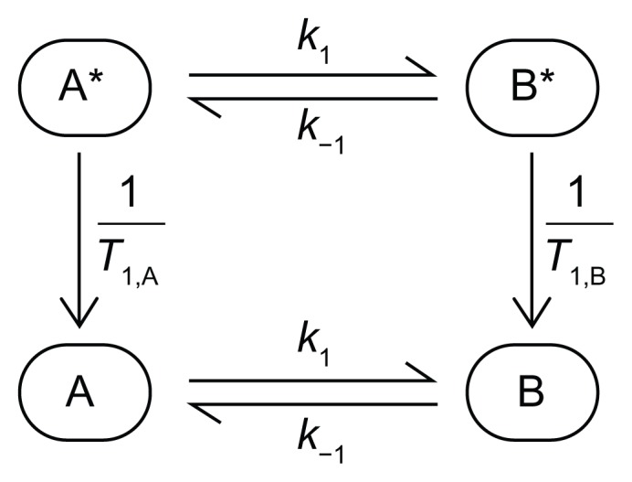
Representation of a simple kinetic model in which molecular species A is converted to B and vice-versa with unitary rate constants k₁ and k₋₁, respectively.

Notes: The * denotes the hyperpolarized molecules that relax to their equilibrium Boltzmann state according to the relaxation time T₁ (subscript A and B denote the corresponding species).

Building a Mathematical Model and Fitting it to Experimental Data

Building the mathematical model

The construction of a realistic mathematical model of the experimental system requires the use of dedicated software such as Matlab or Mathematica; in our research group, we use the latter. The model is built as a ‘function’ inside a module, thus enabling the use of locally defined variables. All the parameters to be evaluated are combined into a vector which becomes the ‘argument’ (input) of the model. This approach allows the ready numerical evaluation of the model. As an illustration, consider the system described in Fig. 4 with the notable parameters whose values must be estimated: T₁, k₁ and k₋₁. Suppose that the function is given the name MODEL, the variables are input in the argument of the function as follows:

$$\begin{array}{c}\text{vector}=\{T_{1,A},T_{1,B},k_1,k_{-1}\};\\ \text{MODEL}[\text{vector}];\end{array}$$

The most important feature in MODEL is the differential rate equations that describe chemical flux in the (bio)chemical reactions. As mentioned above, two sets of equations must be written: the first set for the hyperpolarized (detected) molecules, and the second set for the cold (non-hyperpolarized) molecules. Then the pools of hot (hyperpolarized) and cold molecules are interconnected by the relaxation of the hot molecules. For the system described in Fig. 4, the relevant differential equations are (these take the form that has been used in tracer exchange enzyme kinetics, and also in earlier studies using magnetization-transfer NMR spectroscopy to study membrane transport processes in cell suspensions):22

$$\begin{array}{l}\frac{dA*}{dt}=-\left(\frac{1}{T_{1,A}}+k_1\right)A*[t]+k_{-1}B*[t]\\ \frac{dB*}{dt}=-\left(\frac{1}{T_{1,B}}+k_{-1}\right)B*[t]+k_{1}A*[t]\\ \frac{dA}{dt}=\frac{A*[t]}{T_{1,A}}-k_{1}A[t]+k_{-1}B[t]\\ \frac{dB}{dt}=\frac{B*[t]}{T_{1,B}}-k_{-1}B[t]+k_{1}A[t]\end{array}$$ (2)

As described in the section on the effect of the read RF pulses, magnetization is decreased in discrete steps by these pulses. Since the system of differential equations may be nonlinear and hence not have a simple analytical solution, we choose to calculate the magnetization after each RF pulse by numerical integration of the differential equations, ie, to carry out the integration over the discrete time intervals between each z-magnetization-sampling RF pulse. Thus, these calculations generate a series of values of all signals for the series of time points (see below for a more detailed explanation). To simulate signal evolution for each reactant during a time course, we employ a loop that has the same number of increments as we have experimental time points (1 NMR spectrum = 1 time point); thus it is necessary to define the time during which the signal freely evolves (no RF pulse). Typically, this time is the inter-FID repetition time (TR). We then solve the set of differential equations over TR using as the initial conditions the magnetizations at the beginning of the new TR interval. The amount of each reactant is cumulatively added to the output matrix. The new initial conditions must be determined, and these depend on the flip angle, α, of the z-magnetization-sampling RF pulse. The hyperpolarized reactants will experience diminution by a factor (1 − cos α) while the non-hyperpolarized molecules will have their amounts increased by this factor. Typically this outcome is expressed in the program as follows:

$$\begin{array}{l}A{*}_0=\text{Cos}[\mathrm{\alpha }]A*[t_{end}]\\ B{*}_0=\text{Cos}[\mathrm{\alpha }]B*[t_{end}]\\ A_0=A[t_{end}]+\left(1-\text{Cos}[\mathrm{\alpha }]\right)A*[t_{end}]\\ B_0=B[t_{end}]+\left(1-\text{Cos}[\mathrm{\alpha }]\right)B*[t_{end}]\end{array}$$ (3)

where t_end denotes the signal at the end of the time interval, and the subscript 0 denotes the initial value for the next numerical-integration period.

At the end of the simulation, the discrete time values and the amounts of the different reactants, including the initial quantities, are output.

Further comments on the model

The readily apparent parameters whose values we seek to estimate are concerned with relaxation and (bio)chemical interconversions. However, any of the parameters appearing in the above description can be estimated in the statistical fitting analysis. Uncertainties exist regarding the value of the z-magnetization-sampling RF pulse as this one is strongly dependent on the electronics of the NMR spectrometer, as well as the ionic composition (electrical conductivity) of the sample-medium. Therefore, the pulse angle can be added as a floating (to be fitted) parameter to the input vector.

For both in vitro and especially for in vivo experiments the model must account for the “arrival time” (delay after injection into the sample or animal) of the hyperpolarized reactant. For the former case, the hyperpolarized molecules are usually injected directly into the sample in NMR magnet, thus constituting a stopped-flow type of experiment. However, because the injection of a solution creates distortion of the magnetic field, the first transients cannot be used in the subsequent data analysis (or alternatively the start of data acquisition can be judiciously delayed). To take this effect into account, a delay parameter can be added to the model as a floated (to be estimated/fitted) parameter. In the case of in vivo experiments, the hyperpolarized solute is typically injected into the tail vein of the animal (rodent) and it travels throughout the circulatory system to reach the organ of interest. This injection is usually not as fast as is achievable in an in vitro experiment. Thus the signal built-up can readily be observed and the arrival time of the chemical at the particular organ must be factored into the model. This is done by modifying the differential equations for the injected hyperpolarized reactant during the time that its signal increases. A kinetic constant k_inj, to simulate the time course of delivery of the compound, is included. Using the previous example and considering that A* is injected, its differential equation during its delivery phase (the first few seconds) is expressed as:

$$\frac{dA*}{dt}=-\left(\frac{1}{T_{1,A}}+k_1\right)A*[t]+k_{-1}B*[t]+k_{inj}$$ (4)

Finally, to check that there are no obvious mistakes in the model, the output data, including all molecules for both hot and cold states are scrutinized for their conservation of mass throughout the simulated time courses.

Fitting the data

Once the model has been composed, it is facile to generate apparent signal evolutions for a set of values of relaxation and kinetic parameters and to compare the predictions with real experimental data. To fit the experimental dataset, we have used an approach based on Markov-chain Monte-Carlo (MCMC) analysis.24,25 Any constraints (on T₁ and k values such as only positive numbers being allowed) are specified in the Mathematica program. Because a detailed description of the fitting method used in our recent work on DNP is beyond the scope of this article, the interested reader is referred to the following references.24,26

Conclusions

We have shown which key parameters need to be taken into account while modeling data from DNP experiments. On one hand, NMR parameters (viz., T₁ or the ‘magnetization-sampling’ RF pulse angle α) must be built into the model to properly describe the intrinsic process of signal attenuation. On the other hand, the total quantity of metabolites must be accounted for when describing the (bio)chemical kinetic processes. The consequence of this is to double the number of differential equations to account for the pools of both hyperpolarized and non-hyperpolarized reactants. We have explained our model-design strategy and how to incorporate all parameters into the model. Extra parameters like an initial transient time (delay) before the start of the reaction(s), or progressive delivery over a finite time interval of hyperpolarized reactant(s), can readily be added to the model by using the basic strategy described here.

References

- 1.Overhauser AW. Polarization of nuclei in metals. Phys Rev. 1953;92(2):411–5. [Google Scholar]
- 2.Carver TR, Slichter CP. Experimental verification of the Overhauser nuclear polarization effect. Phys Rev. 1956;102(4):975–80. [Google Scholar]
- 3.Ardenkjær-Larsen JH, Fridlund B, Gram A, et al. Increase in signal-to-noise ratio of >10,000 times in liquid-state NMR. Proc Natl Acad Sci U S A. 2003;100(18):10158–63. doi: 10.1073/pnas.1733835100. [DOI] [PMC free article] [PubMed] [Google Scholar]
- 4.Golman K, Ardenkjær-Larsen JH, Petersson JS, Mansson S, Leunbach I. Molecular imaging with endogenous substances. Proc Natl Acad Sci U S A. 2003;100(18):10435–9. doi: 10.1073/pnas.1733836100. [DOI] [PMC free article] [PubMed] [Google Scholar]
- 5.Golman K, in ‘t Zandt R, Thaning M. Real-time metabolic imaging. Proc Natl Acad Sci U S A. 2006;103(30):11270–5. doi: 10.1073/pnas.0601319103. [DOI] [PMC free article] [PubMed] [Google Scholar]
- 6.Day SE, Kettunen MI, Gallagher FA, et al. Detecting tumor response to treatment using hyperpolarized 13C magnetic resonance imaging and spectroscopy. Nat Med. 2007;13(11):1382–7. doi: 10.1038/nm1650. [DOI] [PubMed] [Google Scholar]
- 7.Gallagher FA, Kettunen MI, Day SE, et al. Magnetic resonance imaging of pH in vivo using hyperpolarized 13C-labelled bicarbonate. Nature. 2008;453(7197):940–3. doi: 10.1038/nature07017. [DOI] [PubMed] [Google Scholar]
- 8.Harris T, Eliyahu G, Frydman L, Degani H. Kinetics of hyperpolarized 13C1-pyruvate transport and metabolism in living human breast cancer cells. Proc Natl Acad Sci U S A. 2009;106(43):18131–6. doi: 10.1073/pnas.0909049106. [DOI] [PMC free article] [PubMed] [Google Scholar]
- 9.Dafni H, Larson PEZ, Hu S, et al. Hyperpolarized 13C spectroscopic imaging informs on hypoxia-inducible factor-1 and Myc activity downstream of platelet-derived growth factor receptor. Cancer Res. 2010;70(19):7400–10. doi: 10.1158/0008-5472.CAN-10-0883. [DOI] [PMC free article] [PubMed] [Google Scholar]
- 10.Brindle KM, Bohndiek SE, Gallagher FA, Kettunen MI. Tumor imaging using hyperpolarized 13C magnetic resonance spectroscopy. Magn Reson Med. 2011;66(2):505–19. doi: 10.1002/mrm.22999. [DOI] [PubMed] [Google Scholar]
- 11.Schroeder MA, Clarke K, Neubauer S, Tyler DJ. Hyperpolarized magnetic resonance: a novel technique for the in vivo assessment of cardiovascular disease. Circulation. 2011;124(14):1580–94. doi: 10.1161/CIRCULATIONAHA.111.024919. [DOI] [PMC free article] [PubMed] [Google Scholar]
- 12.Reed GD, Larson PEZ, Morze Cv, et al. A method for simultaneous echo planar imaging of hyperpolarized 13C pyruvate and 13C lactate. J Magn Reson. 2012;217:41–7. doi: 10.1016/j.jmr.2012.02.008. [DOI] [PMC free article] [PubMed] [Google Scholar]
- 13.Wiesinger F, Weidl E, Menzel MI, et al. IDEAL spiral CSI for dynamic metabolic MR imaging of hyperpolarized [1–13C]pyruvate. Magn Reson Med. 2012;68(1):8–16. doi: 10.1002/mrm.23212. [DOI] [PubMed] [Google Scholar]
- 14.Reynolds S, Patel H. Monitoring the solid-state polarization of 13C, 15N, 2H, 29Si and 31P. Appl Magn Reson. 2008;34(3):495–508. [Google Scholar]
- 15.Cudalbu C, Comment A, Kurdzesau F, et al. Feasibility of in vivo 15N MRS detection of hyperpolarized 15N labeled choline in rats. Phys Chem Chem Phys. 2010;12(22):5818–23. doi: 10.1039/c002309b. [DOI] [PubMed] [Google Scholar]
- 16.Lumata L, Jindal AK, Merritt ME, Malloy CR, Sherry AD, Kovacs Z. DNP by thermal mixing under optimized conditions yields >60 000-fold enhancement of 89Y NMR signal. J Am Chem Soc. 2011;133(22):8673–80. doi: 10.1021/ja201880y. [DOI] [PMC free article] [PubMed] [Google Scholar]
- 17.Lumata L, Merritt ME, Hashami Z, Ratnakar SJ, Kovacs Z. Production and NMR characterization of hyperpolarized 107,109Ag complexes. Ang Chem Int Ed. 2012;51(2):525–7. doi: 10.1002/anie.201106073. [DOI] [PMC free article] [PubMed] [Google Scholar]
- 18.Kettunen MI, Hu DE, Witney TH, et al. Magnetization transfer measurements of exchange between hyperpolarized [1-13C]pyruvate and [1-13C]lactate in a murine lymphoma. Magn Reson Med. 2010;63(4):872–80. doi: 10.1002/mrm.22276. [DOI] [PubMed] [Google Scholar]
- 19.Zierhut ML, Yen YF, Chen AP, et al. Kinetic modeling of hyperpolarized 13C1-pyruvate metabolism in normal rats and TRAMP mice. J Magn Reson. 2010;202(1):85–92. doi: 10.1016/j.jmr.2009.10.003. [DOI] [PMC free article] [PubMed] [Google Scholar]
- 20.Witney TH, Kettunen MI, Brindle KM. Kinetic modeling of hyperpolarized 13C label exchange between pyruvate and lactate in tumor cells. J Biol Chem. 2011;286(28):24572–80. doi: 10.1074/jbc.M111.237727. [DOI] [PMC free article] [PubMed] [Google Scholar]
- 21.Harrison C, Yang C, Jindal A, et al. Comparison of kinetic models for analysis of pyruvate-to-lactate exchange by hyperpolarized 13C NMR. NMR Biomed. 2012;25(11):1286–94. doi: 10.1002/nbm.2801. [DOI] [PMC free article] [PubMed] [Google Scholar]
- 22.Kuchel PW, Chapman BE. NMR spin exchange kinetics at equilibrium in membrane transport and enzyme systems. J Theor Biol. 1983;105(4):569–89. doi: 10.1016/0022-5193(83)90220-5. [DOI] [PubMed] [Google Scholar]
- 23.Puckeridge M, Pagès G, Kuchel PW. Simultaneous estimation of T1 and the flip angle in hyperpolarized NMR experiments using acquisition at non-regular time intervals. J Magn Reson. 2012;222(1):68–73. doi: 10.1016/j.jmr.2012.06.006. [DOI] [PubMed] [Google Scholar]
- 24.Kuchel PW, Naumann C, Puckeridge M, Chapman BE, Szekely D. Relaxation times of spin states of all ranks and orders of quadrupolar nuclei estimated from NMR z-spectra: Markov chain Monte Carlo analysis applied to 7Li+ and 23Na+ in stretched hydrogels. J Magn Reson. 2011;212(1):40–6. doi: 10.1016/j.jmr.2011.06.006. [DOI] [PubMed] [Google Scholar]
- 25.Puckeridge M, Chapman BE, Conigrave AD, Kuchel PW. Quantitative model of NMR chemical shifts of 23Na+ induced by TmDOTP: applications in studies of Na+ transport in human erythrocytes. J Inorg Biochem. 2012;115(SI):211–9. doi: 10.1016/j.jinorgbio.2012.03.009. [DOI] [PubMed] [Google Scholar]
- 26.Andrieu C, de Freitas N, Doucet A, Jordan MI. An introduction to MCMC for machine learning. Mach Learn. 2003;50(1–2):5–43. [Google Scholar]