Computational Recipe for Efficient Description of Large-Scale Conformational Changes in Biomolecular Systems

Abstract

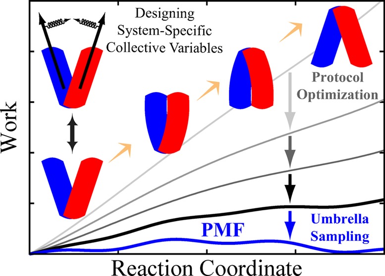
Characterizing large-scale structural transitions in biomolecular systems poses major technical challenges to both experimental and computational approaches. On the computational side, efficient sampling of the configuration space along the transition pathway remains the most daunting challenge. Recognizing this issue, we introduce a knowledge-based computational approach toward describing large-scale conformational transitions using (i) nonequilibrium, driven simulations combined with work measurements and (ii) free energy calculations using empirically optimized biasing protocols. The first part is based on designing mechanistically relevant, system-specific reaction coordinates whose usefulness and applicability in inducing the transition of interest are examined using knowledge-based, qualitative assessments along with nonequilirbrium work measurements which provide an empirical framework for optimizing the biasing protocol. The second part employs the optimized biasing protocol resulting from the first part to initiate free energy calculations and characterize the transition quantitatively. Using a biasing protocol fine-tuned to a particular transition not only improves the accuracy of the resulting free energies but also speeds up the convergence. The efficiency of the sampling will be assessed by employing dimensionality reduction techniques to help detect possible flaws and provide potential improvements in the design of the biasing protocol. Structural transition of a membrane transporter will be used as an example to illustrate the workings of the proposed approach.

1. Introduction

With relentless advances in supercomputing, and rapid expansion of the number of structurally characterized macromolecules, molecular dynamics (MD) has evolved into a standard tool for studying biomolecular phenomena.^1,2 While experimental techniques often provide either a high-resolution static or a low-resolution dynamic picture of the molecular phenomena, MD simulations can violate this “uncertainty relation” between spatial and temporal resolutions and provide a dynamic, yet detailed view at an atomic level.^3,4 Conventional MD simulations, however, suffer from poor conformational sampling, preventing one from achieving an accurate description of conformational ensembles and free energy landscapes. Despite the ever-increasing capability of supercomputers, the time scale limitation remains a great challenge; the typical time scale of an atomistic MD simulation of biomolecular systems is much smaller than those required to describe most biologically relevant molecular phenomena. For instance, many biological processes, e.g., active membrane transport, which rely on large-scale conformational changes of a protein, occur on time scales of milliseconds or longer.⁵

Over the past few decades, various enhanced sampling techniques have been formulated to address the time scale problem in biomolecular simulations.⁶⁻¹⁶ These methods are often tested initially on relatively small representative molecular systems, e.g., dialanine peptide.^10,17−21 A handful of these methods are used routinely for the study of more realistic biomolecular systems. From a practical perspective, however, applying many of these advanced methods to complex biological systems is challenging.

Ideally, MD simulations can be used to characterize thermodynamic and kinetic properties of a biomolecular system/process. From a numerical perspective, these quantities require certain integrations over a high-dimensional phase space—or configuration space, with making certain assumptions—which in turn require a large set of independent and identically distributed samples. One can also reduce the many-dimensional atomic coordinate space into a much smaller space simply by considering the constraints associated with the steric factors (e.g., covalent bonds).²² Nonetheless, the curse of dimensionality remains unbeatable unless additional assumptions or simplifications are made.

One particular premise that many free energy calculation and path optimization methods rely on is the existence of a low-dimensional manifold on which lie most of the relevant conformations visited by a system during a structural transition, i.e., an intrinsic manifold embedded in the atomic coordinate space.^22,23 The intrinsic manifold premise relies mostly on the high cooperativity of the biomolecules; the motions of different parts of a protein, for instance, are correlated along the transition pathway(s).²²

The identification of the “true” reaction coordinate (or the committor function²⁴) which, in principle, parametrizes the intrinsic manifold becomes particularly important for inferring kinetic information from configurational integrations. Note that one may need to make several assumptions with regard to the committor function (e.g., velocity independence) and the transition tube (e.g., localization) in order to connect a computable potential of mean force (PMF) to transition rates.²⁵

In the context of PMF calculations, the task of identifying the intrinsic manifold is often done in an ad-hoc manner. In many free energy methods, e.g., umbrella sampling (US)¹⁶ or its nonequilibrium variations (such as many flavors of driven^6,7 or adaptive-bias techniques^10,26−29), a low-dimensional collective variable is defined based on the a priori knowledge of the system. The assumption is that biasing the system along a “good” reaction coordinate will result in samples that are distributed (although not statistically correct, due to the bias) along the correct transition tube.

In order to identify the intrinsic manifold more systematically, one may use a statistical learning method such as principal component analysis (PCA),³⁰ isomap,²² or diffusion map.^23,31 Dimensionality reduction techniques such as PCA and its nonlinear counterparts are often used to analyze MD trajectories.^22,23,30,32 These have also been used in conjunction with enhanced sampling techniques such as metadynamics,^33,34 adaptive biasing force,³⁵ and US.¹⁸

Many techniques take advantage of the intrinsic manifold premise without an explicit use of a conventional dimensionality reduction technique. For instance, path-optimization techniques (e.g., different flavors of the string method^11,17,36) or path-optimizing free energy techniques³⁷⁻³⁹ rely on the existence of a localized transition tube. These methods simplify the choice of collective variables by allowing the use of many atomic coordinates or collective variables since the sampling is assumed to converge to the relevant regions of the configuration space (i.e., the transition tube).

The approach discussed here can be categorized as an ad-hoc dimensionality reduction method in that the reaction coordinates and biasing protocols are designed through an empirical search. Moreover, our approach heavily relies on our knowledge of the system under study in order to limit the conformational sampling to the relevant regions of the phase space while keeping the calculations reliable and accurate. The approach and the underlying methodology are particularly tuned toward systems that undergo large-scale and complex conformational changes. We take advantage of available structural information for the system (e.g., the crystal structures of the end states even if they only provide partial information on the atomic coordinates) to identify a set of system-specific reaction coordinates that can be used to induce conformational transitions. By combining several techniques within an empirical framework, the proposed approach could narrow the gap between advanced sampling techniques and realistic applications. The general framework of this approach is based on two equally important and novel elements: (i) empirical design of nonequilibrium driving protocols and (ii) converting the optimized nonequilibrium protocols into equilibrium biasing protocols for free energy calculations.

This paper is organized as follows. In section 2, we discuss our proposed approach with an example illustrating the workings of the approach. Section 3 will detail some of the technical aspects of the approach for the interested practitioners, while the last section is reserved for a brief summary and conclusion.

2. Combining Nonequilibrium and Equilibrium Approaches

It is believed that functionally important, large-scale conformational motions of proteins are associated with a hierarchy of substates and time scales.⁴⁰ Consider a complex conformational transition in a rugged free energy landscape involving multiple metastable states and several/many characteristic time scales. Under these conditions, any MD-based quantification of thermodynamic properties such as free energy goes hand in hand with some simplification (e.g., selecting a few reaction coordinates). Even in methods that allow for simultaneous application of many collective variables (e.g., string method^17,36), the choice of initial conformations/pathways is crucial to what the final results converge to (e.g., free energy or transition pathway).

Recognizing these issues, we propose an approach that takes into account, in a balanced manner, all the factors determining the final results including (i) the reaction coordinates used for biasing, (ii) the initial conformations/pathways used to initiate the sampling, (iii) the enhanced sampling techniques, and (iv) the posthoc analysis methods used to quantify the results and estimate the uncertainties.

Figure 1 illustrates the overall flow of our proposed approach. Briefly, there are multiple mostly qualitative (I) and mostly quantitative (II) stages involved. Our approach hinges on efficiently combining these stages in a balanced manner. Although an accurate quantitative result such as a free energy profile is much more desirable than a qualitative description, a reliable free energy map is often too costly to be obtained. On the other hand, the more we know about a system and its approximate free energy landscape, the better we can design an efficient free energy simulation. Therefore, one may improve the efficiency of free energy simulations by taking advantage of qualitative (but reliable) information on the system. In particular, experimental clues combined with fast nonequilibrium techniques provide an appropriate framework for this approach.

Figure 1.

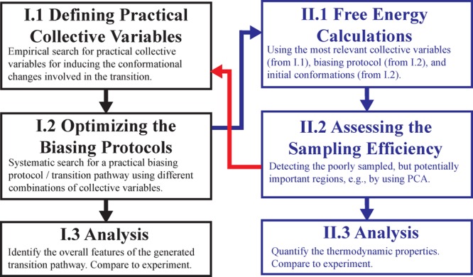
Proposed approach for the study of large-scale conformational changes in proteins. (I) Qualitative component using nonequilibrium driven simulations (left panels). (II) Quantitative component using free energy calculations (right panels). Although the conclusions drawn from the analysis of the results (stages I.3 and II.3) may be used at any point (depending on the assessed accuracy), iterating the process improves the accuracy of such conclusions.

Given the complexity of conformational free energy landscapes, an iterative sampling approach seems necessary in which the results of each iteration (from imperfect sampling) are used to design better reaction coordinates, to generate better initial conformations, and to better sample the relevant regions of the configuration space.

2.1. Nonequilibrium Driven Simulations

One of the fastest ways to generate a physically meaningful pathway between two known conformations for a molecular system is to use a time-dependent external force. This approach is employed most prominently in simulation techniques such as steered⁷ and targeted⁶ MD which use a harmonic restraint with a center (defined in a collective variable space) moving according to a given schedule.

An important disadvantage of these methods is that the resulting trajectories are “far from equilibrium;” these methods often violate laws of equilibrium thermodynamics as well as those laws formulated for local-equilibrium, near-equilibrium, and steady-state nonequilibrium thermodynamics (e.g., Onsager reciprocity relations and fluctuation–dissipation theorem⁴¹). In other words, inferring information with regard to the behavior of the system at equilibrium from trajectories generated by steered or targeted MD is not straightforward. Fortunately, externally driven, far-from-equilibrium systems too follow certain laws such as “nonequilibrium work relations.”⁴²⁻⁴⁵

Nonequilibrium work relations are powerful tools in describing the behavior of systems driven far from equilibrium by the external variation of a parameter. In an MD simulation, a time-dependent biasing potential defined in terms of a collective variable can be used to drive the system from an initial state toward a final one. Here, the collective variable acts as a control parameter, varied according to a protocol. Methods such as steered⁷ and targeted⁶ MD, therefore, fall into the category of nonequilibrium driven simulations.

Nonequilibrium work relations have been used in many applications to numerically estimate the free energies based on the nonequilibrium work measurements;^46,47 however, the use of these relations is not limited to free energy calculations. In principle, nonequilibrium work relations can be used to estimate any equilibrium macroscopic quantity from nonequilibrium driven trajectories.^43,48 Due to the sampling limitations, such a generalization is not necessarily of practical use; however, one may find certain quantities that can be estimated at a modest computational cost.

As an example, one may estimate the relative transition rates of competing pathways using nonequilibrium work measurements.⁴⁹⁻⁵¹ The relative transition rates of different paths can be used to estimate their relative importance without requiring an accurate estimate of the whole free energy landscape.^49,51 Suppose that different “hypothetical” mechanisms associated with a conformational transition can be attributed to distinct transition tubes in a particular collective variable space. The relative importance of each tube can be estimated using nonequilibrium work measurements based on biasing protocols that guide the system via these transition tubes.⁴⁹⁻⁵¹

Along the same lines, one may measure the nonequilibrium work along different transition pathways, not for a quantitative description of the transition rates but rather to simply assess, in a qualitative and relative manner, the practicality of different nonequilibrium protocols.^47,52,53 This semiquantitative ad hoc work analysis is one of the novel features of our nonequilibrium approach that will be discussed here. However, we can only provide some general rules on how to employ the method and how to improve the biasing protocols. The approach is intrinsically empirical and knowledge-based and will not result in any improvements without some a priori knowledge of the molecular system under study.

2.1.1. Assessment of Biasing Protocols Using Nonequilibrium Work Measurements

In principle, the probability of each transition tube (which is proportional to its associated transition rate) can be measured using work measurements given adequate sampling.^49,51 However, the presence of distinct work trends between the most relevant transition tube (which is dominant when the system is not biased) and other hypothetical transition tubes (which are disfavored when the system is not biased) can simplify the calculations.^47,52−54 Note that due to the nonequilibrium nature of the simulations, one cannot make reliable statements based on single trajectories. However, the trend of the work (determined from repeated simulations) can be used to compare different transition paths/mechanisms.

In order to explore the transition tubes, one may define a set of relevant reaction coordinates to reduce the configuration space to a coarse coordinate space with a clear distinction between different states of the system including initial, final, and different hypothetical intermediate states. Let us assume that, using these reaction coordinates, one designs two nonequilibrium driven protocols 1 and 2, each sampling a particular transition tube by driving the system from state A to B through transition tubes 1 and 2, respectively. Consider a scenario in which there is a clear trend in the work profiles generated by the two protocols such that protocol 1 always results in a nonequilibrium work profile whose largest peak is lower than the largest peaks of all work profiles generated by protocol 2. Under such a scenario—which is not uncommon—one may quickly identify which hypothetical transition mechanism is worth investigating (mechanism 1 in this case).

We note that any parameter involved in the biasing protocol (e.g., simulation time) can influence the trend of the work. One can simplify the comparison by keeping some of these parameters constant between different protocols associated with different mechanisms/pathways. Ideally, only one “explanatory” variable⁵⁵ should be varied among the protocols to avoid complications in the comparison. In other words, the protocols should be designed such that they all differ only in one parameter. Here we consider the trend of the work as a “response” variable;⁵⁵ any parameter that varies between different biasing protocols could be generally considered a candidate “explanatory” variable which might substantiate the difference in the work trends. For instance, if the two protocols use two essentially different collective variables (e.g., a distance versus an angle), the comparison will be nontrivial; the different work trends could be due to the way the collective variables are defined (not due to the difference of the paths taken).

Using different collective variables exploring similar pathways will be justified if it provides a way of empirically finding the optimum protocol to sample a given pathway. Therefore, one may take advantage of nonequilibrium driven MD and nonequilibrium work relations in an empirical manner, in order to set the stage for a more systematic investigation. In section 3, we will discuss a few typical techniques for fast comparison of candidate protocols that are not necessarily designed to represent different transition tubes. We show how nonequilibrium work measurements can be used to assess the quality of a protocol and more importantly to compare it to other protocols in order to define an optimal set of collective variables and/or force constants.

2.2. Equilibrium Free Energy Calculations

With a multidimensional free energy landscape calculated, one can identify and quantify the free energy minima and saddle points. Unfortunately, this is currently too ambitious of a goal for an MD-based study of large-scale conformational changes. Most free energy calculations thus effectively sample a localized region of the configuration space. Using a knowledge-based approach in choosing the biasing protocol involved in the sampling and employing an empirical work minimizer in order to optimize the biasing protocol may increase the chance of sampling along the “relevant” transition tube. The idea is not exclusive and may be combined with other approaches. For instance, our best nonequilibrium trajectory can be relaxed into an even more optimized pathway using the string method.^11,17 Note that the choice of the initial pathway is crucial to the convergence of path-finding algorithms such as the string method.⁵⁶⁻⁵⁸

With appropriate changes, a nonequilibrium driven scheme can be converted into a free energy calculation method. For instance, repeating the nonequilibrium driven simulations (preferably in a bidirectional scheme) may be used to reconstruct the PMF.^44,59 Unfortunately, this approach is often associated with a slow convergence. We recently proposed an adaptive-bias variation of nonequilibrium driven MD which takes advantage of an iterative adaptive biasing potential in order to speed up the convergence.⁶⁰ Nonetheless, here we will base our approach on the most popular free energy calculation method, i.e., US.¹⁶ Due to its similarity to steered MD, an US protocol can be conveniently designed based on a fine-tuned steered MD protocol by replacing the time-dependent driving potential with a time-independent biasing potential, as will be discussed in more detail in section 3.

2.2.1. Bias-Exchange Umbrella Sampling

US¹⁶ combined with the weighted histogram analysis method (WHAM)⁶¹ is a standard free energy calculation scheme for reconstructing the PMF along a given reaction coordinate. Employing the method to large-scale transitions, however, is often challenging, and simple biasing protocols (e.g., using the-root-mean-square deviation (RMSD) from a target structure as the reaction coordinate) usually produces unreliable estimates for free energies. By using system-specific reaction coordinates and sampling around reliable transition pathways (obtained using the approach described above), one may significantly improve the sampling.

Sampling a continuous portion of the configuration space along a reaction coordinate becomes particularly more likely when US is used in conjunction with a replica-exchange scheme,^8,9 termed here bias-exchange umbrella sampling (BEUS)⁵⁴ (also known as window-exchange or replica-exchange umbrella sampling^9,62,63).

In replica-exchange MD,^8,9 each replica is associated with a different value of a given property whose periodic exchange between the replicas based on an “exchange rule” accelerates the exploration of the phase space. Temperature is the most commonly used property to exchange between the replicas which accelerates the sampling of all degrees of freedom somewhat blindly. Alternatively, one can exchange, in a time-dependent⁶⁴ or time-independent⁶² manner, biasing potentials in a “bias-exchange” scheme to specifically accelerate the sampling of the degrees of freedom most relevant to the transition of interest. Temperature- and bias-exchange simulations could also be combined to yield a better convergence.^47,65−68

The mixing of the replicas in the bias-exchange method guarantees the continuity of the conformational space sampled (at least for each individual replica), thereby yielding a more reliable free energy profile for the process. Note that due to the large number of degrees of freedom in most biomolecular systems, it is virtually impossible to sample a continuous conformational space if the simulations were to run independently as in a conventional US scheme.

The efficiency of the BEUS simulations depends on (i) the definition of collective variables, (ii) the choice of initial conformations, and (iii) the choice of the window/umbrella parameters (i.e., centers and force constants). The choice of the collective variables (and initial conformations) can be improved, e.g., by using nonequilibrium simulations as described above. The umbrella parameters can be optimized iteratively using short runs with the goal of achieving roughly similar rates of exchange between neighboring replicas. With certain assumptions, one may also use a more systematic approach to adjust these parameters.^62,63,69,70 Along with the factors mentioned above, the choice of the exchange rules plays a role in the efficiency of the BEUS scheme as discussed elsewhere.^71,72

2.2.2. Reweighting and Analysis of BEUS Data

The trajectories generated by (BE)US MD simulations are biased by a known biasing scheme that can be used to reweight the samples, recover the correct statistics, and extract (by proper integration) information with regard to the transition mechanism. However, a suboptimal reaction coordinate for biasing can easily result in a poor sampling and unreliable information. It is thus important to assess the quality of sampling^68,71,73,74 before interpreting the results.

The conventional US/WHAM approach^16,61 often assumes a priori knowledge of a good reaction coordinate which is used for both biasing and PMF reconstruction. However, in the absence of a perfect reaction coordinate, the sampling in the degrees of freedom other than the one used for sampling is important for both determining the reliability of the results and designing better reaction coordinates. The data collected from (BE)US simulations along an imperfect reaction coordinate may not give us an accurate free energy profile, but it can be used, particularly in an iterative manner, to arrive at better reaction coordinates and thus reliable free energies.

Given the computational cost of the (BE)US simulations, it is important to recognize that a flexible analysis framework may be necessary in order to (i) maximize the amount of acquired information on the transition mechanism and (ii) detect sampling flaws and possibly identify better reaction coordinates. In both cases, the sampling along the degrees of freedom orthogonal to the one used for biasing plays a key role. Some of these degrees of freedom are too slow or too fast; the former cannot be identified, and the latter will be sampled properly. Special care must be taken, however, with regard to those events which occur neither too slowly nor too quickly. The degrees of freedom associated with such events will be sampled poorly, thus needing to be identified and taken into account in interpreting the results.

One of the techniques that simplifies much of the analysis required to derive information on the degrees of freedom other than the one used for sampling is the nonparametric reweighting,⁷⁵⁻⁷⁸ which assigns a weight to each individual conformation sampled. A weighted histogram or other weighted statistical analysis methods can thus be performed once the weights are estimated. The PMF (or weighted histogram) can be reconstructed in terms of any arbitrary measurable quantity; however, the PMF reconstructed along a poorly sampled coordinate will not be accurate. Assessing the quality of sampling along different coordinates is thus important in order to (i) determine the reliability of the results and (ii) diagnose the sampling. For a discussion on several variations of nonparametric reweighting schemes, see section S1 in the Supporting Information. These variations include both maximum-likelihood^75,77 and Bayesian⁷⁸ estimators.

One important set of reaction coordinates to investigate is the knowledge-based set as defined in stage I.1 (Figure 1). One may measure those collective variables that potentially represent significant mechanistic features. The PMF along such reaction coordinates is naturally only accurate within the well-sampled region. An unweighted histogram/PMF can be used to readily distinguish between well-sampled and poorly sampled regions. Note that the importance of the continuous sampling is evident here as a gap along any reaction coordinate (not just the one used for biasing) indicates unreliable statistics. A systematic approach in detecting discontinuities (or outliers) is clustering, e.g., using pairwise RMSDs. A relatively less costly clustering approach involves PCA⁷⁹ (based on the biased BEUS samples). A pairwise clustering can then be performed using a metric defined only based on the significant PCs (i.e., those with significant contributions to the variance).

In an n-dimensional BEUS simulation, the first n PCs are likely to correlate well with the n reaction coordinates used for biasing. Detecting more than n significant PCs indicates the existence of slow degrees of freedom orthogonal to the reaction coordinates used for sampling. Note that for reliable sampling, all slow degrees of freedom must be included in the biasing scheme. A similar idea has been introduced by Ferguson et al. based on a nonlinear dimensionality reduction technique.¹⁸

The importance of the degrees of freedom orthogonal to the order parameter for efficient and robust sampling has been known for quite a while, which is related to the so-called “Hamiltonian lagging” problem.⁸⁰ Our approach to addressing this issue is to iteratively (i) detect hidden free energy barriers which are in the conformational space orthogonal to the reaction coordinate and (ii) incorporate the slow orthogonal degrees of freedom in the biasing protocol. An alternative approach is the “orthogonal space random walk”⁸¹⁻⁸³ (or more recently “orthogonal space tempering”⁸⁴) which simultaneously enhances the sampling in the reaction coordinate space and its generalized force space.

2.3. Example—Large-Scale Structural Transition in a Membrane Transporter

In order to illustrate the effectiveness and some of the technical aspects of the methodology introduced here in the context of a concrete biomolecular system, we will take advantage of a set of simulations we have recently performed on a membrane transporter in an explicit lipid/water environment.⁵⁴ We set out for an extensive search on conformational ensemble and structural transitions of MsbA, a bacterial exporter of the ATP-binding cassette (ABC) superfamily.⁵⁴ We note that our recent report on this membrane transporter⁵⁴ did not describe the methodological details of the approach (the subject of the present paper) and only emphasized our findings from a mechanistic perspective and in the context of the function of ABC exporters. Here, we provide in-depth discussion and analyses that were mostly omitted in our recent report due to the difference in the scope and emphasis.⁵⁴

An ABC exporter consists of two nucleotide-binding domains (NBDs) and two transmembrane domains (TMDs).⁸⁵ The NBDs dimerize upon ATP binding and dissociate due to its hydrolysis.^86,87 MsbA is a unique ABC exporter in that its structure has been crystallized in three distinct conformations, including an outward-facing (OF) and two inward-facing (IF) conformations with varying degrees of cytoplasmic opening, termed IF-closed (IF-c) and IF-open (IF-o), respectively. The OF structure was solved to 3.7 Å (PDB: 3B60), while both IF structures are solved at a lower resolution (4.5 Å), therefore allowing for only C^α positions to be determined (PDB: 3B5X and 3B5W).⁸⁸

Experimental evidence supports an IF↔OF transition during the transport cycle^87,89 such that the transporter alternates between IF and OF states (“alternating access” mechanism⁹⁰); however, there is no consensus on what exactly these two states are and what intermediate conformations are involved. From a computational perspective, conventional unbiased MD simulations cannot be used directly to study the IF↔OF transition, due to their limited time scales. However, the crystal structures of MsbA provide a great framework for the study of the transition by designing relevant collective variables and biasing protocols inducing the transition.

2.3.1. Reaction Coordinates

As pointed out earlier, we can use any source of information on the end states to design global reaction coordinates that best capture the molecular motions involved in a transition. For the case of MsbA, the available crystal structures⁸⁸ provide such a source of information. Although the crystal structures of MsbA (IF-c and IF-o, in particular) are of low resolution, they can be used to identify the bundling of the helices and their orientations in different states, based on which we defined the following reaction coordinates: α, the relative orientation of the TMD helices describing the cytoplasmic opening; β, the relative orientation of the TMD helices describing the periplasmic opening; γ, the relative orientation of the two NBDs (see Figure 2). Note that α and β are associated with the TMD conformational changes and can be used to induce opening of the cytoplasmic side and closing of the periplasmic side, respectively. On the other hand, γ is associated with the NBD conformational changes and can be used to induce the twisting of the NBDs.

Figure 2.

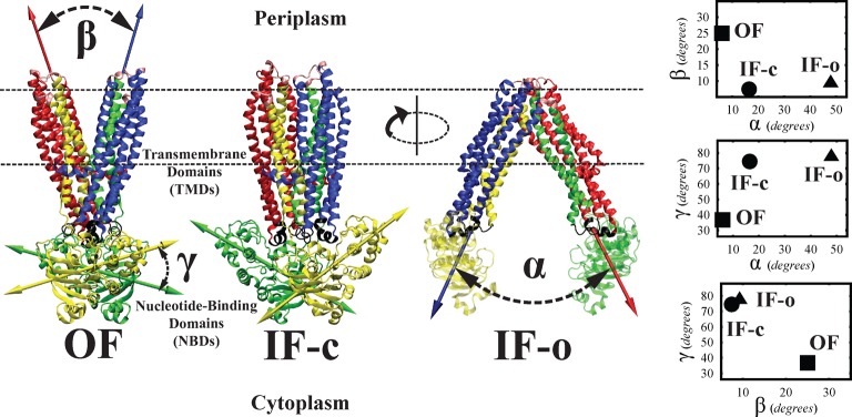
Cartoon representation of MsbA crystal structures in OF, IF-c, and IF-o conformations along with the definitions of reaction coordinates α, β, and γ. The panels on right show the projections of the OF (square), IF-c (circle), and IF-o (triangle) crystal structures onto (α,β), (α,γ), and (β,γ) spaces. Color Code: NBD^cis/trans is colored yellow/green, and TMD bundles B₁ (TM_1,2^cis, TM_4,5 helices), B₂ (TM_1,2^trans, TM_4,5), B₃ (TM_3,6^cis), and B₄ (TM_3,6) are colored blue, red, yellow, and green, respectively. In the OF conformation, the roll axes of bundles B₁/B₄ (G_β^cis) and B₂/B₃ (G_β) are colored blue and red, respectively, to illustrate the definition of β. In the IF-o conformation, the roll axes of bundles B₁/B₃ (G_α^cis) and B₂/B₄ (G_α) are colored blue and red, respectively, to illustrate the definition of α. The roll axes of NBD^cis/trans in the OF and IF-c conformations are colored yellow/green to illustrate the definition of γ.

Triplet (α,β,γ) describes the global conformational features of the MsbA transporter in a 3D coarse coordinate space. One may think of many other collective variables to be used for biasing, e.g., the distance between the mass centers of NBDs (d_NBD). d_NBD was actually used in some of our simulations as well, but to simplify our discussion, we will only focus on α, β, and γ reaction coordinates here.

2.3.2. Nonequilibrium Protocols

We used the equilibrated OF structure of apo MsbA to initiate several nonequilibrium driven MD simulations using different protocols driving the protein toward the IF-o state, including conventional targeted MD simulations and orientation-based driven simulations. We have previously reported on “one-stage” targeted MD simulations based on the IF-o structure.⁵⁴ Here, we used “two-stage” targeted MD simulations, targeting the OF state toward IF-c in the first stage, and IF-c state toward IF-o in the second stage. Figure 3 compares the results of a typical one-stage targeted MD protocol (red) to its two-stage counterpart (blue).

Figure 3.

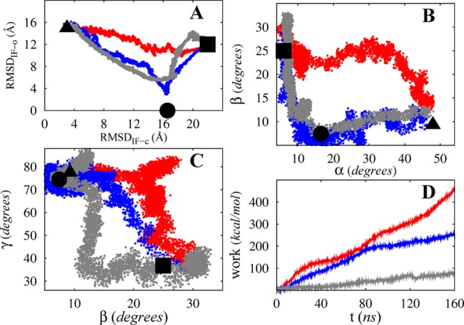
Comparison of the results of one-stage (red) and two-stage (blue) targeted MD protocols with our (α,β,γ)-based protocol (gray). The three 160 ns trajectories are projected onto the (RMSD_IF-o,RMSD_IF-c), (α,β), and (β,γ) spaces in panels A, B, and C, respectively, while panel D shows the nonequilibrium, transferred work measured along the trajectories. Note that square, circle, and triangle represent OF, IF-c, and IF-o crystal structures, respectively.

In the trajectories resulting from the one-stage targeted MD protocols the cytoplasmic opening occurs consistently prior to the closing of the extracellular side resulting in a channel-like intermediate that is simultaneously open to both cyto- and periplasm (see Figure 3B). This clearly contradicts the alternating access mechanism and questions the relevance of these trajectories (knowledge-based assessment). In addition, the final conformation of one-stage targeted MD simulations is found to be unstable in subsequent equilibrium simulations, during which the structure opens to both cyto- and periplasmic sides.

The two-stage targeted MD simulations typically result in better trajectories in that (i) the intermediate conformation does not violate the alternating access mechanism (see Figure 3B) and (ii) the equilibration of both final and intermediate conformations (i.e., the ones at the end of first and second stages) results in locally stable conformations. More interestingly, one can identify a clear difference in the trend of nonequilibrium work of the two protocols: two-stage simulations always require less work than one-stage ones when the same simulation time is used (see Figure 3D for an example).

Introducing the IF-c structure as an intermediate in the targeted MD simulations proved to be helpful in improving the protocol both qualitatively (more consistent with the alternating access mechanism) and semiquantitatively (based on nonequilibrium work). Nevertheless, the amount of nonequilibrium work still appears to be too high, and it is unlikely that the resulting trajectory provides a reliable pathway that can be used for further quantitative studies, especially for free energy calculations. We thus use a more systematic approach to sample the reaction-path ensemble of this complex transition.

We use different combinations of α, β, and γ reaction coordinates to induce the OF → IF transition. One may design many different biasing protocols using these reaction coordinates. Assuming the major changes in α, β, and γ occur in discrete stages, a systematic study will be feasible with only six distinct classes of protocols (all possible orders of these reaction coordinates). The results show that one particular biasing order (β → γ → α) consistently requires less amount of work than others. Interestingly, comparing this protocol with RMSD-based protocols reveals great improvement. Figure 3 compares examples of trajectories obtained from our optimum orientation-based protocol and targeted MD simulations.

Although the nonequilibrium work provides a semiquantitative tool for comparing different protocols, a knowledge-based assessment of the resulting trajectories is necessary, particularly if one decides to perform free energy calculations based on these trajectories. For instance, it is quite likely that a protocol involving a short nonequilibrium simulation results in internal conformational distortions such as helix unwinding. This artifact was observed in some of our shorter simulations (not shown in Figure 3). In addition to the secondary structure, one may monitor other conformational features of the internal domains for a knowledge-based assessment (see Figure S3 for examples). We note that certain local conformational changes (e.g., a side-chain flipping) may be achieved only through further relaxation of conformations during an unbiased or biased equilibrium simulation (e.g., during follow-up BEUS simulations).

2.3.3. Free Energy Calculations

One may use our optimum biasing protocol and its resulting nonequilibrium trajectory to initiate a set of BEUS simulations to estimate the PMF. One may think of this process as transforming a nonequilibrium work profile which is dominated by a dissipative term (e.g., the gray line in Figure 3) to an equilibrium free energy profile. Within the methodological framework introduced in this paper, equilibrium free energy calculations can be thought of as the final step in the process of removing the dissipative term from work. In other words, nonequilibrium protocol optimization reduces the amount of dissipative work and makes the subsequent free energy calculations more efficient and less costly; however, the optimized work profiles are likely to be dominated by a dissipative term.

Given the multistage nature of our MsbA protocol, we set out to perform free energy calculations only on the final stage (i.e., conformational change along α between IF-c and IF-o conformations). These calculations are particularly useful in identifying the resting state of IF MsbA by characterizing the degree of cytoplasmic opening for the nucleotide-free apo MsbA in its IF state. Figure 4 compares the PMF along α between the values associated with IF-c and IF-o crystal structures⁸⁸ (i.e., α_IF-c ≈ 16° and α_IF-o ≈ 48°, respectively) to the work profiles associated with the nonequilibrium simulations discussed above (i.e., one-stage and two-stage targeted MD as well as the optimized protocol) as plotted against α and offset by the work at α_IF-c ≈ 16°. Here, the PMF was estimated from BEUS MD free energy calculations along α as the reaction coordinate using 22 replicas each running for 24 ns, with degrees of opening ranging from 13° to 49° in the α space.

Figure 4.

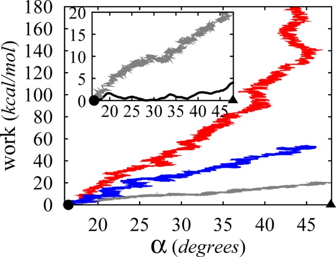
Nonequilibrium, transferred work required by 160 ns MD simulations performed using one-stage (red) and two-stage (blue) targeted MD as well as the optimized protocol (gray), as plotted against α and offset by the work at α_IF-c ≈ 16°. The work profiles are obtained from the same simulations described in Figure 3, and shown only within the α = 16–48° (≈ α_IF-c–α_IF-o) range. Inset: Nonequilibrium work obtained from the optimized protocol (gray) compared to the PMF along α as obtained from the BEUS simulations (see Figure 5). Note that the circle and triangle represent crystal structures IF-c and IF-o, respectively.

Figure 5A shows the reconstructed PMF along α within the entire sampled range. There exists a local minimum around α ≈ 16° (the value associated with the IF-c crystal structure), while no free energy basin is discernible around α ≈ 48° (the value associated with the IF-o crystal structure⁸⁸), suggesting that the large opening of the cytoplasmic end might be an artifact of crystal contacts. Nonetheless, the deepest minima in the α space are in the 26–32° range forming a basin that is associated with an IF conformation resembling the crystal structures of a homologous transporter protein (P-glycoprotein),⁹¹⁻⁹³ which are obtained at higher resolutions. The overall picture emerging from the PMF calculations along α represents MsbA as a fairly flexible structure in its resting state in the absence of nucleotides and substrates. We note that while these observations support the relevance of our PMF results, we cannot rule out the possibility of a more stable open conformation corresponding to the IF-o crystal structure which is not captured in our sampling.

Figure 5.

PMF of apo MsbA in the IF state along different reaction coordinates (A, α; B, γ; C, PC1; and D, PC2). The PMF is obtained from BEUS MD simulations performed using an α-based biasing protocol and estimated using a Gibbs sampler (see Supporting Information). Principal components were constructed from all C^α atoms of the protein from all conformations used for the PMF estimations. The mean values and the error bars are estimated from 100 PMFs generated by bootstrapping.

PMF in Other Dimensions

Although α is the single most relevant reaction coordinate (among the ones designed) to capture the conformational changes of MsbA associated with the opening of the cytoplasmic side in the IF state, more information can be extracted from the BEUS simulations performed along α by reconstructing the PMF along other reaction coordinates. Among them, γ is of particular interest, not only from a mechanistic perspective but also to assess sampling efficiency. This is due to a flexibility associated with γ; diffusion along γ is fast enough to be sampled during 24 ns of BEUS simulations. However, sampling along γ is not homogeneous since it was not included in the biasing protocol. Figure 5B shows the PMF along γ. Noting that in all initial conformations γ is between 60° and 80°, it is not surprising to have the smallest estimated errors around this region (i.e., better sampling) while the largest estimated errors are for the regions with γ < 35° (i.e., poor sampling).

From a sampling efficiency assessment perspective, instead of choosing arbitrary reaction coordinates to analyze, one may use PCA.³⁰ We thus performed PCA based on all C^α atoms of the protein using all conformations sampled by BEUS simulations. Table 1 shows the fraction of variance explained by first four PCs along with the correlation between the PCs with a select number of other reaction coordinates. As expected, PC1 correlates well with α, which was used for sampling (correlation coefficient of 0.97). The PMF along PC1 (Figure 5C) resembles the PMF along α as well. However, PC1 only explains about 2/3 of the variance. PC2, on the other hand, correlates strongly with γ (correlation coefficient of 0.82), and the PMF along PC2 (Figure 5D) resembles that along γ. PC2 explains about 22% of the variance.

Table 1. Correlation between Select Collective Variables and Principal Components Based on All BEUS Data.

	PC1	PC2	PC3	PC4
fraction of variancea	65.6%	22.5%	2.1%	1.6%
correlation coefficientb
α	0.97	0.30	–0.06	–0.15
β	–0.05	0.28	0.13	–0.03
γ	–0.14	0.82	–0.01	0.14
dNBD	0.98	0.33	0.03	0.04
RMSDOF	0.90	0.54	0.05	–0.02
RMSDIF–c	0.98	0.01	–0.06	0.01
RMSDIF–o	–0.94	–0.45	0.01	0.03

^aFraction of (unweighted) variance explained by each principal component.

^bPearson correlation coefficient between a principal component (column) and a collective variable (row).

The PCA results suggest that biasing the system along α alone might not be enough to achieve good sampling in the PC2 space (which correlates strongly with γ). Meanwhile, the PMF along the (α,γ) space, although not accurate in some regions, may provide clues on the mechanism of transition (Figure 6A). γ tends to “un-twist” in the intermediate α range, a behavior also observed in our earlier equilibrium simulations.⁵⁴

Figure 6.

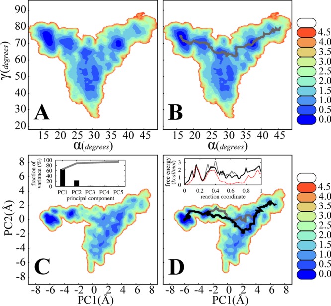
(A) Contour plot of the PMF in the (α,γ) space (in kcal/mol) as obtained from the α-based BEUS simulations. (B) Same as A with a pathway generated by the LFEP algorithm.⁹⁴ (C) Same as A but in the (PC1,PC2) space (as defined in Figure 5). Inset: the fraction of variance (of unweighted BEUS-generated conformations) “explained” by the first five principal components (bars) and their cumulative value (gray line). (D) Same as C with two pathways generated by the LFEP algorithm. Inset: free energy along the two LFEP-generated pathways (black and gray) compared to the PMF along α (red). An IF-c → IF-o reaction coordinate is defined by transforming either α (red) or arc length of the path (black and gray) to make the comparison between the three easier.

In the next iteration, one may use a 2D BEUS MD simulation involving both α and γ in order to ensure good sampling along both dimensions. If the 2D BEUS is not feasible—it could be too computationally demanding—the resulting approximate 2D PMF provides a way of identifying important pathways, e.g., the pathway shown in Figure 6B, found using the lowest free energy path (LFEP) algorithm,⁹⁴ and restraining the replicas along a 1D path. If multiple competing pathways coexist, one may perform several 1D BEUS simulations, instead of a 2D one. Obviously the 2D BEUS simulation will be more informative but also computationally more costly. Better sampling along γ not only improves the PMF estimate along γ but also makes our free energy estimate along α more accurate. However, note that the definition of free energy along α will depend on the way γ was incorporated into the protocol, i.e., a second dimension for sampling or a degree of freedom to be restrained.

Figure 6C,D show the PMF in the (PC1,PC2) space. The fraction of variance explained by the first five principal components and their cumulative value are also shown. The free energy along the two LFEP-generated pathways as obtained from our reconstructed PMFs is compared to the PMF along PC1. The 1D PMF is significantly lower than the free energy along either pathway, where the sampled region is elongated along PC2 due to the presence of multiple metastable states.

Identifying Potentially Significant Residues

Besides PCA and other analyses targeting the global features of the conformations, one may be interested in more local conformational changes, particularly those correlating with large-scale conformational changes. A 2D PMF can be constructed in terms of α (or PC1), representing the global conformational change, and any quantity of interest representing a more localized change.

As an example, here we discuss a potentially significant salt bridge between residues D252 and K299. Figure 7 plots the 2D PMF in the (α,χ_D252–K299) space in which χ_D252–K299 counts the number of D252–K299 salt bridges formed in the cis and trans monomers. Conformations associated with several minima are presented in Figure 7. IF-c and IF-c* are both similar to the IF-c crystal structure; however, they differ in their number of salt bridges. IF-o* and IF-o^† are also similar to the IF-o crystal structure (although both less open), exhibiting different numbers of salt bridges.

Figure 7.

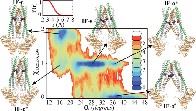
Contour plot of the PMF in the (α,χ_D252–K299) space (in kcal/mol) as obtained from the α-based BEUS simulations. χ_D252–K299 smoothly counts the number of D252–K299 salt bridges (in the cis and trans monomers). χ_D252–K299 = χ(r_{D252^cis–K299^cis}) + χ(r_{D252^trans–K299^trans}), and r_A–B is the distance between (i) the mass centers of the side-chain oxygen atoms of residue A (D252) and (ii) the side-chain nitrogen atom of residue B (K299). Inset: A smooth step function χ(r) used to quantify the formation/breakage of a salt bridge based on r_{D252^cis/trans–K299^cis/trans}. Select conformations associated with several minima are presented in a cartoon representation. TM₅ (green) and TM₆ (orange) helices are highlighted along with D252 (red) and K299 (blue) residues in van der Waals surface representation.

The 2D PMF reveals a strong (nonlinear) correlation between the two global and local quantities α and χ_D252–K299. The larger the α, the less likely it is for the salt bridges to form; however, it turns out that the largest basin (associated with IF-s) which spans over a large α range is associated with an asymmetric salt-bridge pattern. This implies that MsbA in the IF state (at least in the apo form) is more likely to have only one of the salt bridges than both or none. This observation is in line with recent experimental work suggesting an asymmetrical TMD arrangement in MsbA.⁹⁵

Beside the mechanistic insight obtained from the 2D PMFs, e.g., the one shown in Figure 7, such multidimensional PMFs can be used more quantitatively to arrive at a better estimate for the transition barrier. Note that the PMF maximum along any collective variable, if estimated accurately, only provides a lower bound to the actual barrier. This is due to the degeneracy associated with collective variables which becomes evident in our example by comparing the PMF along α with that in the (α,χ_D252–K299) space. There appears to be an approximately 2-kcal/mol barrier around α ≈ 20° in the 1D PMF (Figure 5A); however, the α ≈ 20° point is associated with both a saddle point (χ_D252–K299 ≈ 1) and a basin (χ_D252–K299 ≈ 2), implying that the 2-kcal/mol estimate is dominated by the free energy of a local minimum and not the transition state. The 2D PMF indicates that the free energy associated with the saddle point at α ≈ 20° is around 4 kcal/mol rather than 2 kcal/mol. Although both 4-kcal/mol and 2-kcal/mol values can be considered as lower-bound estimates for the free energy barrier, the 4-kcal/mol estimate is a larger lower-bound, which makes it more informative. Note that, however, there is a trade-off between the accuracy and precision since including more dimensions in PMF reconstruction increases the uncertainty of the results due to limited sampling.

3. Technical Considerations

In section 2, we gave an overview of our proposed scheme to combine several sampling techniques in order to optimize the reliability and relevance of free energy calculations. Here, we will discuss some of the more technical aspects of the approach which could be of particular interest to MD practitioners. Although some of the techniques described here are already known to practitioners, as referenced throughout the discussion, certain practical difficulties arise—or become more serious—when one tries to combine different techniques. The emphasis here is on having a balanced approach toward addressing such practical issues by taking into account the entire process of designing, performing, and analyzing the simulations.

3.1. Nonequilibrium Approach

Nonequilibrium work measurements can be used for a qualitative comparison of different protocols, as described in section 2. However, such comparisons are limited to the sampled transition mechanisms and cannot rule out the possibility of alternative transition mechanisms that are either not sampled or sampled only poorly due to the use of a particular biasing protocol. Another important limitation arises when multiple transition protocols are found with similar trends of nonequilibrium work. If there is a clear trend in work profiles of different mechanisms favoring a number of paths over the others, one can make general qualitative statements about their relative importance; however, the transition paths with similar trends of work cannot necessarily be considered similarly important. For these cases, longer simulations or more iterations might establish a difference in their trends of nonequilibrium work.

3.1.1. Empirical Protocol Optimization

Despite the considerations mentioned above, one may take advantage of nonequilibrium driven MD simulations and nonequilibrium work measurements in an empirical manner as an efficient way to optimize the biasing protocols. We note that before assessing the quality of a protocol based on the amount of work, one needs to determine whether or not the employed protocol is effective in inducing the transition of interest. This may be a trivial task for simple molecular systems, but in the presence of many metastable states, it is quite likely for the system to get trapped in an irrelevant metastable state without ever getting close to the product. The rule of thumb is that once the system is steered along the designed reaction coordinate, followed by a careful equilibration, the product must be locally stable while verifiably resembling the target structure. The careful equilibration here includes (i) restraining the system around the final target, (ii) slow removal of the restraint, and (iii) unrestrained equilibration. In cases in which the target is not a well-known state, our low-resolution knowledge of the target may be used; however, the stability of the product should be established before performing costly computations such as free energy calculations.

Choice of Force Constant

The amount of nonequilibrium work might be sensitive to the choice of force constant when a harmonic bias is used. The force constant needs to be large enough to induce the transition. If the force constant is too large, however, the simulation could become unstable, and the molecular system could undergo deformation or distortion. Within these limits, any force constant may be used to induce the transition of interest; however, choice of the force constant will influence the amount of dissipation. Nonequilibrium work measurements may be used in order to find an optimum value for force constant in an empirical manner. We take advantage of the fact that different force constants result in different work distributions; thus, one may find an optimum force constant which typically (or on average) results in a lower work. See section S2 for a more detailed discussion and an example for this use of work measurements.

Definition of Collective Variables

Suppose that one is interested in inducing a particular conformational transition such as an interdomain orientational change. A “measure” that identifies the desired orientational changes can be easily defined. However, a practical collective variable needs to meet additional requirements. For instance, it should induce the desired conformational change without distorting the system, that is, without taking the system through irrelevant molecular configurations (e.g., unlikely, high-energy states). If several collective variables satisfying this criterion are available, one may use nonequilibrium work measurements in a semiquantitative manner to choose the best one. Thus, one can try different definitions and compare the results, first, by a qualitative knowledge-based assessment of the conformations sampled and, if there is no clear preference, by comparing the work profiles.

Similarly, one may use qualitative comparison of work profiles (along with knowledge-based comparison of the generated trajectories) in order to optimize the choice of atoms directly affected by the biasing potential. For instance, either all heavy atoms, all backbone atoms, or only C^α atoms can be subjected to a biasing potential to induce an orientational change in a helical domain. Nonequilibrium work measurements again provide a basis for optimizing the details of a protocol in a systematic fashion.

3.2. System-Specific Reaction Coordinates

In order to induce a conformational transition, it is often relevant to define a set of collective coordinates⁹⁶⁻⁹⁹ such that by applying appropriate forces on the system, one can vary these collective variables and change the conformation of the system. Any measure/metric distinguishing between different conformations can be used for the analysis of a trajectory; however, it does not necessarily make a practical collective variable suitable for biasing/driving a system from one state toward another. Metrics used for the analysis are often chosen to quantify certain properties in an intuitive manner, but they do not need to be, for instance, differentiable. On the other hand, a collective variable has to be well-behaved to be used in a biasing potential since its gradient and time derivative, for instance, are needed to calculate the biasing force and work, respectively.

One particular collective variable that is widely used in the context of structural transition of proteins is RMSD. Although using the RMSD from a target structure as a collective variable (e.g., in a targeted MD⁶ simulation) has proven useful, the method has its own pitfalls and limitations. RMSD is associated with both extreme degeneracy and large entropy loss¹⁰⁰ (for large and small values of RMSD, respectively). The trajectory generated by targeted MD represents a pathway along which the RMSD decreases almost monotonically and nearly linearly. Another limitation that reduces the flexibility of the method to a great extent is its high sensitivity to the quality/resolution of the target structure. In addition, a targeted MD simulation typically requires a large amount of work to induce a transition, thus making the interpretation of its results difficult in the context of nonequilibrium work relations.

Other conventional collective variables such as distance and radius of gyration have their own limitations in inducing complex structural transitions. Collective variables such as RMSD and radius of gyration can be considered special cases of a “generalized distance” which has been studied with regard to some of its features (e.g., its entropy loss) when used in a biasing potential.¹⁰⁰

One particular feature that seems to best describe a variety of large-scale conformational changes in proteins is semirigid-body domain orientational changes. There are several ways of defining a collective variable that quantifies an orientation-based conformational change. Among them, the orientation quaternion technique^54,101−103 has proven successful as a well-behaved, flexible method for defining system-specific collective variables, specifically aimed at inducing interdomain orientational changes.

Note that here we use the term system-specific reaction coordinates or collective variables for definitions that rely on our knowledge of the conformational changes involved in a transition. If the conformational changes are spatially localized (e.g., a side-chain flipping or a salt-bridge formation/breakage), one may use relatively simple techniques to define a reaction coordinate on a select number of atoms. If the conformational change is global, more advanced collective variables such as the orientation quaternion may be needed to induce the transition of interest. The selection of atoms (grouping of domains, bundling of helices, etc.) in the definition of the collective variables is again a knowledge-based component. We note that when a local conformational change triggers a global conformational change, using collective variables defined on a limited number of atoms may prove more useful in inducing the transition. Using combinations of (generalized) distance-based and/or orientation-based collective variables may be necessary in order to induce a complex global transition.

3.2.1. Orientation Quaternion

Suppose that the relative orientation of two molecular domains change during a transition. The angle between the two domains can be defined as a simple geometric angle based on the mass centers of three groups of atoms (three-group definition). Similarly the arccosine of the dot product of principal axes (usually the roll axes) of two groups of atoms can be used to define the orientation angle (vector-based definition).

Unfortunately, using a simple three-group definition of an angle to induce a global conformational change often results in undesired deformations of the protein. Using the principal axes is associated with certain technical difficulties as well; e.g., the three principal axis components may interchange during the simulation due to conformational changes. We will discuss an alternative technique to define orientation-based collective variables, namely, the orientation quaternion^54,101−103 which has been recently implemented in several MD packages by Fiorin et al.¹⁰³ This technique allows for a flexible and reliable definition of system-specific collective variables, specifically aimed at inducing interdomain orientational changes.

The orientation quaternion,¹⁰² often used for “optimal superposition” in computational biology,¹⁰¹ is a tool to deal with the so-called “absolute orientation” problem. Suppose that for a set of N atoms (labeled 1 ≤ k ≤ N), we have two different sets of measurements: {x_k} and {y_k}. To simplify the problem, we assume both sets have been already shifted to bring their barycenters to the origin (optimum translation). To find the optimum rotation to superimpose {y_k} on {x_k}, we introduce “pure quaternions” x_k and y_k whose vector parts are x_k and y_k, respectively. A quaternion is a four-component vector that can be considered as a composite of a scalar and an ordinary vector, or as a complex number with three different imaginary parts. A quaternion whose scalar part is zero is called pure (reminiscent of pure imaginary numbers). The optimal rotation can be parametrized by a unit quaternion, q̂ that minimizes ⟨∥q̂x_kq̂* – y_k∥²⟩ in which ⟨·⟩ denotes an average over k, q* is the conjugate of q, and ∥q∥² ≡ qq* (see ref (101) for more details). The optimal rotation unit quaternion (or orientation quaternion) q̂ can be written as (cos(θ/2), sin(θ/2)û) in which θ and û (a unit vector) are the optimum angle and axis of rotation, respectively.

As a collective variable, an orientation quaternion can be used not only to monitor rotational changes but also to apply force (which is proportional to the gradient of the quaternion) on the system in a practical way to induce the desired rotational changes. Suppose that we are interested in inducing a particular rotation—given by its axis of rotation (unit vector û) and its target angle of rotation θ_target—on a particular segment of a biomolecule, e.g., part of a helix, an entire helix, or a bundle of helices. This can be done by using a time-dependent harmonic potential similar to steered MD in spirit:

1

Here, q_ref({x_k}) is the optimum orientation quaternion to superimpose {x_k} on a reference set {x_k^ref}. The reference could be the initial, target, or any other structure. Here, to simplify the notations, we assume the reference is the same as the initial structure. Q(t) ≡ (cos(θ(t)/2), sin(θ(t)/2)û) is a unit quaternion that is varied externally, providing the center of the harmonic potential at time t during a simulation (0 ≤ t ≤ T). If the reference is the same as the initial structure, θ(0) and θ(T) can be set to 0 and θ_target, respectively. Once we have Q(0) and Q(T), we can use different interpolation methods to determine Q(t). A simple method is varying θ(t) linearly, which is a special case of the spherical linear interpolation (Slerp) method.¹⁰⁴ The particular method discussed here—implemented by Fiorin et al.¹⁰³—is based on the linear interpolation of the quaternion Q(t), using the current and final centers, followed by its normalization at each time step. Finally Ω(p̂,q̂) is the length of the geodesic between two points on the unit sphere, transformed by p̂ and q̂ from an arbitrary point on the unit sphere. An approximate estimate for Ω(p̂,q̂) is known to be arccos(|p̂·q̂|) in which p̂·q̂ is the inner product of p̂ and q̂.

The nonequilibrium work along a trajectory generated by the quaternion-based biasing protocol (eq 1) can be measured via

2

which is the accumulated work at time t. The nonequilibrium, transferred work¹⁰⁵ can also be measured by subtracting U_B(q_ref({x_k}), t) – U_B⁰ from the accumulated work, in which U_B is the biasing potential measured at t = 0. One can collect the biasing potential (U_B(q_ref,t)) and its partial time derivative (∂U_B(q_ref,t)/∂t) based on the instantaneous q_ref at time t. For the particular q_ref schedule, Q(t) that comes from the linear interpolation of the quaternion (Q′(t + Δt) = Q(t) + (Q(T)–Q(t))Δt/(T–t)) followed by its normalization (Q(t + Δt) = (Q′(t + Δt)/∥Q′(t + Δt)∥), one can show:

3

4

Examples of Orientation-Based Collective Variables

We use our transporter example to demonstrate how orientation quaternions can be used to induce rotational changes. Let us recall the definition of α and β (defined on the TMD helices) as well as γ (defined on the NBDs). Suppose TM_i^cis and TM_i denote the ith transmembrane helix of the two monomers (labeled cis and trans, arbitrarily) and consider four relatively rigid bundles, B₁ (TM_1,2^cis, TM_4,5 helices), B₂ (TM_1,2^trans, TM_4,5 helices), B₃ (TM_3,6^cis helices), and B₄ (TM_3,6 helices), colored in Figure 2 blue, red, yellow, and green, respectively. α describes the angle between two groups of bundles B₁/B₃ (or G_α^cis) and B₂/B₄ (or G_α). On the other hand, β describes the angle between B₁/B₄ and B₂/B₃ (or G_β^cis and G_β, respectively). γ is simply the twist angle between the two NBDs.

The bundling of the helices and the grouping of the bundles as explained here are clearly inspired by the crystal structures of MsbA.⁸⁸ In order to induce conformational changes along α, β, or γ, one may define several orientation quaternions based on (i) individual helices, (ii) different bundles of helices, or (iii) segments of helices and even combine them in different ways. We have discussed this empirical process in section S2 (see Supporting Information). Our empirical process led us to use six orientation quaternions as collective variables to describe the three-dimensional (α,β,γ) space including (q_α^cis, q_α, q_β^cis, q_β, q_γ^cis, q_γ). For each angle two collective variables are defined on the two sides of the angle. q_α^cis and q_α are the orientations of the two groups of bundles G_α^cis and G_α, respectively. Similarly, q_β^cis and q_β are the orientations of G_β^cis and G_β, respectively. q_γ^cis/trans is the orientation quaternion defined on NBD^cis/trans.

3.3. Free Energy Calculations

The connection between harmonic-based nonequilibrium driven MD and harmonic-based (BE)US is quite evident. One can easily design a number of time-independent biasing potentials along the time-dependent biasing potential as the umbrella window potentials and use the generated nonequilibrium conformations close to the window centers as initial conformations. The force constants and the window centers may be adjusted in order to achieve sufficient overlapping of the sampled windows and, in the BEUS scheme, reasonable mixing of the replicas.

It is shown that placing the window centers equidistantly defined with a proper thermodynamic metric (i.e., along the geodesic) minimizes the variance in the estimate of free energies and optimizes the mixing of replicas (within a given protocol).⁶⁹ Similarly, within the linear response regime, a nonequilibrium driven protocol can be optimized by minimizing the dissipation or the thermodynamic divergence by moving along the geodesic with a constant speed.¹⁰⁶ The two are indeed related and one may use the information obtained from one (e.g., the thermodynamic metric) to optimize the other. In other words, the overlap (mixing) required for the convergence of (BE)US simulations is related to the average dissipative work measured from the driven simulations. Roughly speaking, one may conclude that the more dissipation that is observed in a driven protocol, the more expensive the free energy calculations from (BE)US simulations would be.

3.3.1. Proposed Sampling Protocol

Suppose that we are interested in sampling the transition between A and B state along the protocol ζ. We propose the following steps to prepare and perform BEUS simulations.

1. Nonequilibrium Driven MD. In order to decrease the risk of discontinuous sampling in BEUS simulations, we propose generating the initial conformations from a continuous trajectory. This can be done using a nonequilibrium driven MD simulation. We assume we have already optimized the protocol ζ. Starting from A, we drive the system along ζ toward B and generate M conformations along the protocol.

2. Parameter Adjustment. Efficiency of the sampling in BEUS simulations relies on both (i) mixing of the replicas and (ii) overlap between the windows. Suppose that the exchange rate between replica i and i + 1 is r_i,i+1 (for i = 1, ..., N – 1, in which N is the number of replicas). The optimum exchange rate R = r_i,i+1 depends on several factors, e.g., the exchange scheme.⁷² However, the flatness of the r_i,i+1 function (i.e., r_i,i+1 = R, where R is constant) is particularly important to achieve an efficient diffusion along the reaction coordinate (assuming no phase transition involved). With regard to the overlap between the windows, a critical criterion (particularly when weak force constants are applied) is that the entire reaction coordinate space must be sampled without any gap. Note that having an equal exchange rate between the replicas does not guarantee a flat sampling along the reaction coordinate. Therefore, when adjusting the parameters, one needs to first make sure that there are no nonexchanging/nonoverlapping windows.

One may use the following procedure prior to production runs of BEUS simulations to prepare the initial conformations and umbrella potentials using a trajectory generated in a prior nonequilibrium simulation:

(a) Take N initial conformations from the M nonequilibrium conformations. At first, one may pick the conformations from equal time intervals.

(b) Based on each conformation i (selected above), identify a center ζ_i along the reaction coordinate. For each umbrella i = 1, ..., N, design a biasing potential (or umbrella potential) U_i restraining ζ around ζ_i with harmonic constant k_i.

(c) Perform short BEUS MD simulations starting with the initial conformations and using the umbrella potentials obtained from steps a and b, respectively.

(d) Iterate steps a to c with different initial conformations (N can be varied as well) and harmonic constants until (i) the exchange rate between any two neighboring replicas was estimated to be in a given range (e.g., 20–40%) and (ii) the ζ space (in a given continuous range) is expected to be sampled without any gap. This process may be done empirically; however, a more automatic process can also be implemented.

3. Production. The final set of initial conformations and umbrella potentials generated above can be used to perform longer BEUS simulations to achieve convergence.

3.3.2. Sampling Efficiency

While the mixing of the replicas in a BEUS scheme decreases the likelihood of discontinuity, it does not fully eliminate it. The continuity of the regions sampled by each replica is evident; however, there could be discontinuity introduced by the initial conformations such that some of the replicas never cross the regions sampled by other replicas. Suppose one picks the initial conformations of a BEUS simulation from several independent simulations or a single simulation much longer than the individual BEUS simulations. This introduces a high risk of nonoverlapping replicas which all sample perfectly well along the reaction coordinate (used for sampling) with a reasonable mixing (in terms of exchange rate), but they never actually cross each other along a degree of freedom orthogonal to the reaction coordinate. Although clustering will detect such problems, it is important to avoid risky choices for initial conformations. We suggest using a single nonequilibrium simulation to generate the initial conformations.

In the conventional US scheme, using weak force constants may result in a higher risk of discontinuous sampling. In the BEUS simulations, however, the discontinuity in the sampling is less likely and the use of weaker force constants is justified as long as they are stiff enough to ensure a continuous sampling free of any gaps. The convergence, however, is typically slower than that in a stiff-spring setting.

Note that using stiff harmonics which result in narrow Gaussian distributions is a straightforward approach to simplify the optimization of US/BEUS parameters.^62,70 However, using stiff harmonics is not necessarily computationally efficient. The narrower the distribution, the larger the number of windows needed for reasonable exchange rate and overlap. On the other hand, a broader distribution may converge slower; thus, the trade-off between the convergence time and number of windows must be considered in choosing the force constants.

Finally, we note that for detecting insufficient sampling and hysteresis along the degrees of freedom orthogonal to the reaction coordinate, one may use techniques such as a pairwise consistency test between the probability distribution of adjacent windows as recently introduced by Zhu and Hummer.¹⁰⁷ For other techniques used to characterize the sampling efficiency, we refer the reader to refs (71), (73), (74), and (108).

3.3.3. Relaxation

Conventional US is a time-independent biasing scheme; thus, the samples generated by each umbrella are assumed to satisfy the detailed balance criterion and have the correct biased Boltzmann distribution. However, the initial conformations are not necessarily selected from the correct distribution. The initial part of US simulations, thus, cannot be used to construct the biased (and subsequently unbiased) distributions and must be discarded. Note that the equilibration process may be longer for weaker biasing potentials since a broader configuration space is accessible. In general, the time scale associated with this conformational relaxation is not known a priori and must be determined a posteriori. For instance, one may discard the samples from an initial period several times longer than the autocorrelation time. Alternatively, one may take advantage of the fact that the sampling during the equilibration period is often inconsistent with the rest of the data and discard (from the beginning) as many samples as possible in order to minimize the posterior error.

In the BEUS scheme, the conformations sampled in a particular umbrella window may belong to different replicas. Unlike the extended ensemble (i.e., all replicas/windows combined), neither individual replica trajectories nor individual (reconstructed) window trajectories satisfy the detailed balance criterion. However, conformations sampled by any given umbrella have the correct biased Boltzmann distribution, assuming the extended ensemble is equilibrated. This implies that in addition to conformational relaxation, another relaxation associated with the diffusion of replicas within the extended ensemble scheme is required. Similar to the conformational relaxation, the replica/window relaxation time scale may be determined a posteriori. Note that one may equilibrate the initial conformations (which may come from nonequilibrium simulations) in a conventional US setting prior to performing the BEUS simulations. In this case, the relaxation of the replicas in the window space is still required.

An estimate for the relaxation time associated with mixing of the replicas can be obtained from the exchange rates.⁷¹ A lower bound for the relaxation time can be estimated from τ₂ ≡ Δt/(1 – λ₂) in which Δt is the effective time between exchange attempts and λ₂ is the second largest eigenvalue of an empirical transition matrix constructed using the exchange rates between the windows.⁷¹ By considering an ideal exchange rate between the windows, one may obtain a lower bound for τ₂. For instance, in a 1D BEUS simulation including N windows/replicas, if the exchange is only attempted between the neighboring windows, one can easily show a flat exchange rate of R results in τ₂ ≈ (N² + 1)/(10R)Δt. We note that we have assumed a stochastic choice of odd–even pairs while the deterministic choice (as was used in our example) is expected to result in faster relaxation.⁷²

Relaxation, Correlation, and Convergence in Our Example

Let us examine our BEUS MD trajectories of MsbA transporter used for sampling along α (see section 2) to estimate the relaxation and correlation times. Note that the two are not the same but related; the former determines the portion of data to be discarded due to nonequilibrium relaxation effects, while the latter is needed for error estimation and convergence assessment.

By constructing the empirical transition matrix, τ₂ was estimated to be about 184 ps, which is close to the estimate from τ₂ ≈ (N² + 1)/(10R)Δt ≈ 180 ps ps. We also explicitly estimated the autocorrelation times associated with different quantities including the window index, select collective variables, and several principal components (Table 2). We estimated the autocorrelation times from the correlation functions using the scheme discussed in ref (73). For a given window, the exchange of the conformations in the BEUS scheme results in apparent decorrelation of the data as compared to conventional US. The autocorrelation time for different quantities was estimated to be around 50 to 500 ps. However, one may notice that the actual trajectories associated with the replicas have much longer autocorrelation times when compared to reconstructed window-based trajectories (see Table 2).

Table 2. Autocorrelation Times (in picoseconds) of the BEUS Trajectories Associated with Different Quantities Including the Window, Select Collective Variables, and First Four Principal Components^a.

	window	α	β	γ	dNBD	PC1	PC2	PC3	PC4
replica	975 ± 30b	1391 ± 70	1492 ± 67	1448 ± 96	783 ± 89	1234 ± 79	1711 ± 54	934 ± 56	1544 ± 71
window		247 ± 17	402 ± 30	175 ± 14	41 ± 36	51 ± 32	136 ± 14	203 ± 41	417 ± 42

^aThe correlations were estimated along (i) an actual trajectory associated with a given replica and (ii) a reconstructed trajectory associated with a given window.

^bThe mean values and standard deviations are given based on 22 trajectories/windows.

The longest autocorrelation time is associated with PC2 which is τ_ac* ≈ 1.7 ns. PC1 and PC2 may be considered the most significant biased and unbiased principal components, respectively. PC2 roughly represents the slowest degree of freedom orthogonal to the reaction coordinate used for biasing. The largest autocorrelation time, which is incidentally associated with PC2, may be used to estimate the statistical inefficiency of the entire data set as g ≈ (2τ_ac*)⁻¹ ≈ 3.4 ns. Alternatively, g can be estimated using the so-called structural decorrelation time¹⁰⁸ which is related to the block-averaging approach.¹⁰⁹ Defining a metric in the (PC1,PC2) space, we estimated τ_dec ≈ 3.2 and 0.5 ns for replica- and window-based trajectories, respectively. With correlation times on the order of nanoseconds, reaching a verifiable convergence may require simulation times on the order of microseconds. The presence of multiple copies of the system and the mixing of the replicas, however, may speed up the convergence considerably. Nonetheless, given these highly correlated data sets, typical of conformational sampling simulations, it is important to use an appropriate technique for error analysis, e.g., Bayesian block bootstrapping¹¹⁰ as discussed in section S1 in the Supporting Information.

4. Conclusion

In summary, here we introduce a computational recipe for efficient description of large-scale conformational transitions in complex molecular systems. The approach combines a set of (i) driven nonequilibrium and (ii) biased equilibrium simulations with similar (but not identical) (i) time-dependent and (ii) time-independent harmonic biasing potentials. The biasing protocols are designed using a knowledge-based approach taking advantage of system-specific collective variables and empirically optimized parameters. The process is knowledge-based in that any structural information available on the end states is used both in the design of the biasing protocols and in their quality assessment. The process is also empirical in that both (i) nonequilibrium and (ii) equilibrium biasing protocols are optimized iteratively by varying the protocol parameters such as collective variables or centers of umbrella windows and assessing the results, e.g., based on nonequilibrium work or rate of exchange. The approach discussed here can be viewed as an ad-hoc dimensionality reduction method in that the sampling is adjusted empirically to restrain the system in a particular region of the configuration space representing relevant transition tube(s) and intrinsic manifold.

Several ideas/techniques described here have been previously discussed/employed by us and others elsewhere, some of which are referenced throughout the paper. The emphasis here is on presenting a coherent picture of the entire process of performing, analyzing, and improving MD simulations aimed at describing functionally relevant, large-scale conformational transitions in complex, realistic biomolecular systems. The process is indeed challenging with diversified, multifaceted issues involved, some of which less appreciated than others. We propose a balanced strategy to combine several techniques within an empirical framework, to address the practical obstacles involved in sampling large-scale conformational changes. Moreover, the current work calls for a more concerted attempt to develop strategies aimed at improving the applicability of advanced sampling techniques to realistic biological problems.

Supporting Information Available

Two nonparametric reweighting schemes for US simulations are described in section S1, and Figure S1 compares their results. Some simulation details with regard to our illustrative example are given in section S2, with Table S1 and Figure S2 providing information on select number of these simulations. Figure S3 reports on internal structural stability of individual domains during select trajectories. This material is available free of charge via the Internet at http://pubs.acs.org/.

The authors declare no competing financial interest.

Funding Statement

National Institutes of Health, United States

References

- Hansson T.; Oostenbrink C.; van Gunsteren W. F. Curr. Opin. Struct. Biol. 2002, 12, 190–196. [DOI] [PubMed] [Google Scholar]
- Karplus M.; McCammon J. A. Nat. Struct. Biol. 2002, 265, 654–652. [DOI] [PubMed] [Google Scholar]
- Karplus M.; Kuriyan J. Proc. Natl. Acad. Sci. U.S.A. 2005, 102, 6679–6685. [DOI] [PMC free article] [PubMed] [Google Scholar]
- Klepeis J. L.; Lindorff-Larsen K.; Dror R. O.; Shaw D. E. Curr. Opin. Struct. Biol. 2009, 19, 120–127. [DOI] [PubMed] [Google Scholar]
- Dornmair K.; Jähnig F. Proc. Natl. Acad. Sci. U.S.A. 1989, 86, 9827–31. [DOI] [PMC free article] [PubMed] [Google Scholar]
- Schlitter J.; Engels M.; Krüger P.; Jacoby E.; Wollmer A. Mol. Simul. 1993, 10, 291–308. [Google Scholar]
- Izrailev S.; Stepaniants S.; Balsera M.; Oono Y.; Schulten K. Biophys. J. 1997, 72, 1568–1581. [DOI] [PMC free article] [PubMed] [Google Scholar]
- Sugita Y.; Okamoto Y. Chem. Phys. Lett. 1999, 314, 141–151. [Google Scholar]
- Sugita Y.; Kitao A.; Okamoto Y. J. Chem. Phys. 2000, 113, 6042–6051. [Google Scholar]
- Laio A.; Parrinello M. Proc. Natl. Acad. Sci. U.S.A. 2002, 99, 12562–12566. [DOI] [PMC free article] [PubMed] [Google Scholar]
- Ren W.; Vanden-Eijnden E.; Maragakis P.; E W. J. Chem. Phys. 2005, 123, 134109. [DOI] [PubMed] [Google Scholar]
- Mitsutake A.; Mori Y.; Okamoto Y. In Biomolecular Simulations; Monticelli L., Salonen E., Eds.; Humana Press: New York, 2013; Methods in Molecular Biology, vol. 924; pp 153–195. [DOI] [PubMed] [Google Scholar]
- Moradi M.; Babin V.; Sagui C.; Roland C. In Biomolecular Simulations; Monticelli L., Salonen E., Eds.; Humana Press: New York, 2013; Methods in Molecular Biology, vol. 924; pp 313–337. [DOI] [PubMed] [Google Scholar]
- Abrams C.; Bussi G. Entropy 2013, 16, 163–199. [Google Scholar]
- Zuckerman D. M.; Woolf T. B. Phys. Rev. E 2000, 63, 016702. [DOI] [PubMed] [Google Scholar]
- Torrie G. M.; Valleau J. P. J. Comput. Phys. 1977, 23, 187–199. [Google Scholar]
- Pan A.; Sezer D.; Roux B. J. Phys. Chem. B 2008, 20, 3432–3440. [DOI] [PMC free article] [PubMed] [Google Scholar]
- Ferguson A. L.; Panagiotopoulos A. Z.; Debenedetti P. G.; Kevrekidis I. G. J. Chem. Phys. 2011, 134, 135103. [DOI] [PubMed] [Google Scholar]
- Mezei M. Mol. Simul. 1989, 3, 301–313. [Google Scholar]
- Crehuet R.; Field M. J. J. Chem. Phys. 2003, 118, 9563–9571. [Google Scholar]
- Jang H.; Woolf T. B. J. Comput. Chem. 2006, 27, 1136–1141. [DOI] [PubMed] [Google Scholar]
- Das P.; Moll M.; Stamati H.; Kavraki L. E.; Clementi C. Proc. Natl. Acad. Sci. U.S.A. 2006, 103, 9887–9890. [DOI] [PMC free article] [PubMed] [Google Scholar]
- Ferguson A. L.; Panagiotopoulos A. Z.; Debenedetti P. G.; Kevrekidis I. G. Proc. Natl. Acad. Sci. U.S.A. 2010, 107, 13597–13602. [DOI] [PMC free article] [PubMed] [Google Scholar]
- E W.; Ren W.; Vanden-Eijnden E. Chem. Phys. Lett. 2005, 413, 242–247. [Google Scholar]
- E W.; Vanden-Eijnden E. Annu. Rev. Phys. Chem. 2010, 61, 391–420. [DOI] [PubMed] [Google Scholar]
- Hummer G.; Kevrekidis I. G. J. Chem. Phys. 2003, 118, 10762–10773. [Google Scholar]
- Huber T.; Torda A. E.; van Gunsteren W. F. J. Comput.-Aided Mol. Des. 1994, 8, 695–708. [DOI] [PubMed] [Google Scholar]
- Babin V.; Roland C.; Sagui C. J. Chem. Phys. 2008, 128, 134101. [DOI] [PubMed] [Google Scholar]
- Markwick P. R. L.; Pierce L. C. T.; Goodin D. B.; McCammon J. A. J. Phys. Chem. Lett. 2011, 2, 158–164. [DOI] [PMC free article] [PubMed] [Google Scholar]
- Amadei A.; Linnsen A. B. M.; Berendsen H. J. C. Proteins: Struct., Funct., Gen. 1993, 17, 412–425. [DOI] [PubMed] [Google Scholar]
- Ferguson A. L.; Panagiotopoulos A. Z.; Kevrekidis I. G.; Debenedetti P. G. Chem. Phys. Lett. 2011, 509, 1–11. [DOI] [PubMed] [Google Scholar]
- Perilla J. R.; Woolf T. B. J. Chem. Phys. 2012, 136, 164101. [DOI] [PMC free article] [PubMed] [Google Scholar]
- Spiwok V.; Lipovová P.; Králová B. J. Phys. Chem. B 2007, 111, 3073–3076. [DOI] [PubMed] [Google Scholar]
- Tribello G. A.; Ceriotti M.; Parrinello M. Proc. Natl. Acad. Sci. U.S.A. 2012, 109, 5196–5201. [DOI] [PMC free article] [PubMed] [Google Scholar]
- Hashemian B.; Millán D.; Arroyo M. J. Chem. Phys. 2013, 139, 214101. [DOI] [PubMed] [Google Scholar]
- Maragliano L.; Fischer A.; Vanden-Eijnden E.; Ciccotti G. J. Chem. Phys. 2006, 125, 024106. [DOI] [PubMed] [Google Scholar]
- Chen M.; Yang W. J. Comput. Chem. 2009, 30, 1649–1653. [DOI] [PubMed] [Google Scholar]
- Díaz Leines G.; Ensing B. Phys. Rev. Lett. 2012, 109, 020601. [DOI] [PubMed] [Google Scholar]
- Cao L.; Lv C.; Yang W. J. Chem. Theory Comput. 2013, 9, 3756–3768. [DOI] [PMC free article] [PubMed] [Google Scholar]
- Ansari A.; Berendzen J.; Bowne S. F.; Frauenfelder H.; Iben I. E.; Sauke T. B.; Shyamsunder E.; Young R. D. Proc. Natl. Acad. Sci. U.S.A. 1985, 82, 5000–5004. [DOI] [PMC free article] [PubMed] [Google Scholar]
- Onsager L.; Machlup S. Phys. Rev. 1953, 91, 1505–1512. [Google Scholar]
- Jarzynski C. Phys. Rev. Lett. 1997, 78, 2690–2693. [Google Scholar]
- Crooks G. E. Phys. Rev. E 2000, 61, 2361–2366. [Google Scholar]
- Hummer G.; Szabo A. Proc. Natl. Acad. Sci. U.S.A. 2001, 98, 3658–3661. [DOI] [PMC free article] [PubMed] [Google Scholar]
- Jarzynski C. Proc. Natl. Acad. Sci. U.S.A. 2001, 98, 3636–3638. [DOI] [PMC free article] [PubMed] [Google Scholar]
- Jensen M. Ø.; Park S.; Tajkhorshid E.; Schulten K. Proc. Natl. Acad. Sci. U.S.A. 2002, 99, 6731–6736. [DOI] [PMC free article] [PubMed] [Google Scholar]
- Moradi M.; Babin V.; Roland C.; Sagui C. J. Chem. Phys. 2010, 133, 125104. [DOI] [PubMed] [Google Scholar]
- Minh D. D. L.; Chodera J. D. J. Chem. Phys. 2011, 134, 024111–024119. [DOI] [PubMed] [Google Scholar]
- Moradi M.; Sagui C.; Roland C. Chem. Phys. Lett. 2011, 518, 109–113. [Google Scholar]
- Moradi M.; Sagui C.; Roland C. J. Chem. Phys. 2014, 140, 034114. [DOI] [PubMed] [Google Scholar]
- Moradi M.; Sagui C.; Roland C. J. Chem. Phys. 2014, 140, 034115. [DOI] [PubMed] [Google Scholar]
- Moradi M.; Babin V.; Roland C.; Darden T.; Sagui C. Proc. Natl. Acad. Sci. U.S.A. 2009, 106, 20746. [DOI] [PMC free article] [PubMed] [Google Scholar]
- Moradi M.; Babin V.; Roland C.; Sagui C. Nucleic Acids Res. 2013, 41, 33–43. [DOI] [PMC free article] [PubMed] [Google Scholar]
- Moradi M.; Tajkhorshid E. Proc. Natl. Acad. Sci. U.S.A. 2013, 110, 18916–18921. [DOI] [PMC free article] [PubMed] [Google Scholar]
- Whitlock M.; Schluter D.. The Analysis of Biological Data; Roberts and Co. Publishers: Greenwood Village, CO, 2009; Analysis of Biological Data Series. [Google Scholar]
- Gan W.; Yang S.; Roux B. Biophys. J. 2009, 97, L8–L10. [DOI] [PMC free article] [PubMed] [Google Scholar]
- Farrell D. W.; Speranskiy K.; Thorpe M. F. Proteins: Struct., Funct., Bioinf. 2010, 78, 2908–2921. [DOI] [PubMed] [Google Scholar]
- Vashisth H.; Maragliano L.; Abrams C. F. Biophys. J. 2012, 102, 1979–1987. [DOI] [PMC free article] [PubMed] [Google Scholar]
- Minh D. D. L.; Adib A. B. Phys. Rev. Lett. 2008, 100, 180602. [DOI] [PMC free article] [PubMed] [Google Scholar]
- Moradi M.; Tajkhorshid E. J. Phys. Chem. Lett. 2013, 4, 1882. [DOI] [PMC free article] [PubMed] [Google Scholar]
- Kumar S.; Bouzida D.; Swendsen R. H.; Kollman P. A.; Rosenberg J. M. J. Comput. Chem. 1992, 13, 1011–1021. [Google Scholar]
- Park S.; Kim T.; Im W. Phys. Rev. Lett. 2013, 108, 108102–108105. [DOI] [PMC free article] [PubMed] [Google Scholar]
- Park S.; Im W. J. Chem. Theory Comput. 2013, 9, 13–17. [DOI] [PMC free article] [PubMed] [Google Scholar]
- Piana S.; Laio A. J. Phys. Chem. B 2007, 111, 4553–4559. [DOI] [PubMed] [Google Scholar]
- Moradi M.; Babin V.; Sagui C.; Roland C. Biophys. J. 2011, 100, 1083–1093. [DOI] [PMC free article] [PubMed] [Google Scholar]
- Moradi M.; Babin V.; Sagui C.; Roland C. J. Phys. Chem. B 2011, 115, 8645–8656. [DOI] [PubMed] [Google Scholar]
- Moradi M.; Babin V.; Sagui C.; Roland C. PLoS Comput. Biol. 2012, 8, e1002501. [DOI] [PMC free article] [PubMed] [Google Scholar]
- Bergonzo C.; Henriksen N. M.; Roe D. R.; Swails J. M.; Roitberg A. E.; Cheatham T. E. J. Chem. Theory Comput. 2014, 10, 492–499. [DOI] [PMC free article] [PubMed] [Google Scholar]
- Shenfeld D. K.; Xu H.; Eastwood M. P.; Dror R. O.; Shaw D. E. Phys. Rev. E 2009, 80, 046705. [DOI] [PubMed] [Google Scholar]
- Sabri Dashti D.; Roitberg A. E. J. Chem. Theory Comput. 2013, 9, 4692–4699. [DOI] [PubMed] [Google Scholar]
- Chodera J. D.; Shirts M. R. J. Chem. Phys. 2011, 135. [DOI] [PubMed] [Google Scholar]
- Lingenheil M.; Denschlag R.; Mathias G.; Tavan P. Chem. Phys. Lett. 2009, 478, 80–84. [DOI] [PubMed] [Google Scholar]
- Chodera J. D.; Swope W. C.; Pitera J. W.; Seok C.; Dill K. A. J. Chem. Theory Comput. 2007, 3, 26–41. [DOI] [PubMed] [Google Scholar]
- Abraham M. J.; Gready J. E. J. Chem. Theory Comput. 2008, 4, 1119–1128. [DOI] [PubMed] [Google Scholar]
- Bartels C. Chem. Phys. Lett. 2000, 331, 446–454. [Google Scholar]
- Habeck M. Phys. Rev. Lett. 2007, 98, 200601. [DOI] [PubMed] [Google Scholar]
- Shirts M. R.; Chodera J. D. J. Chem. Phys. 2008, 129, 124105. [DOI] [PMC free article] [PubMed] [Google Scholar]
- Tan Z.; Gallicchio E.; Lapelosa M.; Levy R. M. J. Chem. Phys. 2012, 136, 144102. [DOI] [PMC free article] [PubMed] [Google Scholar]
- Ding C.; He X. K-means Clustering via Principal Component Analysis. In Proceedings of the Twenty-first International Conference on Machine Learning (ICML-04), Banff, Canada, 2004; Brodley C., Ed.; ACM: New York, 2004; pp 29–38. [Google Scholar]
- Kollman P. A.; Pearlman D. A. J. Chem. Phys. 1989, 91, 7831–7839. [Google Scholar]
- Zheng L.; Chen M.; Yang W. Proc. Natl. Acad. Sci. U.S.A. 2008, 105, 20227–20232. [DOI] [PMC free article] [PubMed] [Google Scholar]
- Zheng L.; Chen M.; Yang W. J. Chem. Phys. 2009, 130, 234105–234114. [DOI] [PubMed] [Google Scholar]
- Min D.; Zheng L.; Harris W.; Chen M.; Lv C.; Yang W. J. Chem. Theory Comput. 2010, 6, 2253–2266. [DOI] [PubMed] [Google Scholar]
- Zheng L.; Yang W. J. Chem. Theory Comput. 2012, 8, 810–823. [DOI] [PubMed] [Google Scholar]
- Davidson A. L.; Dassa E.; Orelle C.; Chen J. Microbiol. Mol. Biol. Rev. 2008, 72, 317–364. [DOI] [PMC free article] [PubMed] [Google Scholar]
- Hollenstein K.; Dawson R. J.; Locher K. P. Curr. Opin. Struct. Biol. 2007, 17, 412–418. [DOI] [PubMed] [Google Scholar]
- Oldham M. L.; Davidson A. L.; Chen J. Curr. Opin. Struct. Biol. 2008, 18, 726–733. [DOI] [PMC free article] [PubMed] [Google Scholar]
- Ward A.; Reyes C. L.; Yu J.; Roth C. B.; Chang G. Proc. Natl. Acad. Sci. U.S.A. 2007, 104, 19005–19010. [DOI] [PMC free article] [PubMed] [Google Scholar]
- Dawson R. J.; Locher K. P. Nature 2006, 443, 180–185. [DOI] [PubMed] [Google Scholar]
- Jardetzky O. Nature 1966, 211, 969–970. [DOI] [PubMed] [Google Scholar]
- Aller S. G.; Yu J.; Ward A.; Weng Y.; Chittaboina S.; Zhuo R.; Harrell P. M.; Trinh Y. T.; Zhang Q.; Urbatsch I. L.; Chang G. Science 2009, 323, 1718–1722. [DOI] [PMC free article] [PubMed] [Google Scholar]
- Jin M. S.; Oldham M. L.; Zhang Q.; Chen J. Nature 2012, 490, 566–569. [DOI] [PMC free article] [PubMed] [Google Scholar]
- Ward A. B.; Szewczyk P.; Grimard V.; Lee C.-W.; Martinez L.; Doshi R.; Caya A.; Villaluz M.; Pardon E.; Cregger C.; Swartz D. J.; Falson P. G.; Urbatsch I. L.; Govaerts C.; Steyaert J.; Chang G. Proc. Natl. Acad. Sci. U.S.A. 2013, 110, 13386–13391. [DOI] [PMC free article] [PubMed] [Google Scholar]
- Ensing B.; Laio A.; Parrinello M.; Klein M. L. J. Phys. Chem. B 2005, 109, 6676–6687. [DOI] [PubMed] [Google Scholar]
- Mittal A.; Böhm S.; Grütter M. G.; Bordignon E.; Seeger M. A. J. Biol. Chem. 2012, 287, 20395–20406. [DOI] [PMC free article] [PubMed] [Google Scholar]
- Go̅ N.; Scheraga J. Chem. Phys. 1969, 51, 4751–4767. [Google Scholar]
- Carter E. A.; Ciccotti G.; Hynes J. T.; Kapral R. Chem. Phys. Lett. 1989, 156, 472–477. [Google Scholar]
- Grubmüller H. Phys. Rev. E 1995, 52, 2893–2906. [DOI] [PubMed] [Google Scholar]
- Rahman A. Phys. Rev. Lett. 1967, 19, 420–421. [Google Scholar]
- Schlitter J.; Swegat W.; Mülders T. J. Mol. Mod. 2001, 7, 171–177. [Google Scholar]
- Coutsias E. A.; Seok C.; Dill K. A. J. Chem. Phys. 2004, 25, 1849–1857. [DOI] [PubMed] [Google Scholar]
- Horn B. K. P. J. Opt. Soc. Am. A 1987, 4, 629–642. [Google Scholar]
- Fiorin G.; Klein M. L.; Hénin J. Mol. Phys. 2013, 111, 3345–3362. [Google Scholar]
- Shoemake K. SIGGRAPH Comput. Graph. 1985, 19, 245–254. [Google Scholar]
- Schurr J. M.; Fujimoto B. S. J. Phys. Chem. B 2003, 107, 14007–14019. [Google Scholar]
- Sivak D. A.; Crooks G. E. Phys. Rev. Lett. 2012, 108, 190602. [DOI] [PubMed] [Google Scholar]
- Zhu F.; Hummer G. J. Comput. Chem. 2012, 33, 453–465. [DOI] [PMC free article] [PubMed] [Google Scholar]
- Lyman E.; Zuckerman D. M. J. Phys. Chem. B 2007, 111, 12876–12882. [DOI] [PMC free article] [PubMed] [Google Scholar]
- Flyvbjerg H.; Petersen H. G. J. Chem. Phys. 1989, 91, 461–466. [Google Scholar]
- Hub J. S.; de Groot B. L.; van der Spoel D. J. Chem. Theory Comput. 2010, 6, 3713–3720. [Google Scholar]
Associated Data
This section collects any data citations, data availability statements, or supplementary materials included in this article.