Theory of Adaptive Optimization for Umbrella Sampling

Abstract

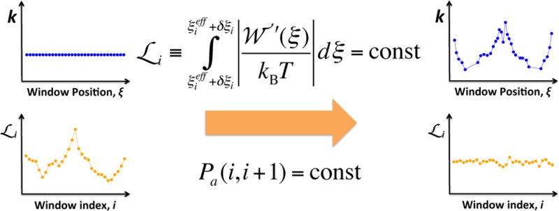
We present a theory of adaptive optimization for umbrella sampling. With the analytical bias force constant obtained from the constrained thermodynamic length along the reaction coordinate, the windows are distributed to optimize the overlap between neighbors. Combining with the replica exchange method, we propose a method of adaptive window exchange umbrella sampling. The efficiency gain in sampling by the present method originates from the optimal window distribution, in which windows are concentrated to the region where the free energy is steep, as well as consequently improved random walk.

Introduction

The potential of mean force (PMF), , as a function of a set of collective variables (CVs), X, can be formally written as

1

where k_B is the Boltzmann constant, T is the temperature, β = (k_BT)⁻¹, δ(z) is a delta function of z, U is the potential energy, and R is a particular configuration of the system. Clearly, the quality of the calculated PMF relies on sampling in the configuration space, {R}. Extensive sampling to obtain the PMF of a complex system is generally difficult even by long molecular dynamics (MD) or Monte Calro (MC) simulations. To better sample along the CVs, especially in steep-PMF regions, the umbrella sampling (US) method¹ has been extensively employed.

There have been many excellent US methods such as the adaptive US,² self-healing US,³ Gaussian mixture adaptive US,⁴ and self-learning adaptive US⁵ to name a few. Except the last one, all the mentioned methods aim to achieve uniform sampling along the CVs by applying an adaptively estimated umbrella potential, which would eventually allow diffusive sampling along the CVs. The last method aims to efficiently determine (multidimensional) free energy landscape around the transition (minimum free energy) pathway by gradually adding windows over low free energy regions.

A typical system for (regular) US simulations consists of a set of windows with umbrella potentials that restrain the CVs near the center of each window, and the simulation data are postanalyzed to calculate the PMF by the weighted histogram analysis method⁶ or the mean force integration.^7,8 For meaningful and efficient US simulations, the overlap between neighboring windows should be sufficient and well controlled. However, there has been no general theory to control the fine overlap because the window centers are system-dependently shifted to the nearest PMF minimum. In order to control the overlap systematically, there should be a quantitative measure of the overlap between a pair of windows. The average acceptance probability P_a is such a measure, which has been originally derived in the theory of replica exchange (REX) methods.⁹⁻¹³P_a describes the overlap between two replicas quantitatively and thus can be directly applied to control the overlap between neighboring windows in US as well.

Recently, there have been efforts in the systematic control of the overlap between windows for the US REX method.^9,14 The first approach in this direction is our previous work,⁹ where we derived a simple relationship between the window force constant k and the window spacing d based on an analytical expression for P_a,

2

where z_opt = 0.8643, which provides the optimal window overlap (i.e., P_a ≈ 0.39) based on the first passage time optimization of REX methods.⁹⁻¹¹ Equation 2 assumes that the PMF has minimal effects on shifts of the window centers. However, when the effect of the PMF becomes significant, the window parameters based on eq 2 are no longer optimal, although it still provides a good initial guess. In addition, the optimal number of windows for efficient US simulations still needs to be determined in an empirical (and system-dependent) manner.

More recently, Dashti and Roitberg¹⁴ proposed a protocol for the optimization of US REX by realizing uniform P_a between replicas, which provides a way to determine where to put windows and how many windows are needed. However, the bias force constant were kept constant and there were only the examples with the fixed number of windows. Without optimization of the bias force constant, the statistical uncertainty in the calculated PMF from US would not be minimized^15,16 and thus its convergence would be slow.

The concept of the thermodynamic length¹⁵⁻¹⁸ provides a rigorous way to minimize the statistical uncertainty by finding a pathway that minimizes the dissipation,^15,16,18 which have been applied in optimization of thermodynamic processes.¹⁹⁻²¹ Using the information theory, the connection between the thermodynamic length and the statistical uncertainty in the free energy calculation has been studied.^15,22−24 In these studies, it has been shown that the statistical uncertainty is minimized when intermediate states are spaced along a minimum distance pathway connecting these states,^15,16,18 which lies on the geodesic connecting the end states.^15,16

In this work, to resolve these general issues in US simulations (efficient sampling with minimal statistical uncertainty), we present a theory of adaptive optimization for umbrella sampling, which is based on equidistant window distribution along the thermodynamic length. Here, we consider one-dimensional US (X = ξ), which can be readily combined with REX methods.^25,26 In the following, the theoretical background for the present method is described. Then, we derive an analytical expression for the optimal (PMF-dependent) bias force constant for US and describe an adaptive optimization that distributes the windows with the optimal bias force constant by constraining P_a. We validate the method and explore its sampling efficiency along the hidden (or orthogonal) degrees of freedom (DOF) by using a toy-model. We then examine the efficacy and the limitation of the present method by applying it to a more realistic (and complicated) example, the assembly of the transmembrane domain of glycophorin A (GpA-TM).

Theoretical Background

Let us consider a system whose canonical distribution of ξ is given by , where . The corresponding (regular) US system consists of N windows and each window i is under the effective potential, U_eff(R) = U(R) + w_i(ξ|ξ_i), where w_i(ξ|ξ_i) is the window potential to restrain sampling of ξ near ξ_i (i = 0, 1,...,N – 1). We assume that the sampling range Λ is continuous (i.e., Λ = [ξ_min, ξ_max]). The sampling range at window i, Λ_i, can be conveniently described by the variance of sampled ξ, σ_ξi², and then, their average for the entire windows becomes σ_ξ = ∑_iσ_ξi²/N. For the uniform sampling along ξ, σ_ξi = σ_ξ² should hold, which is equivalent to the minimization of the total variance, ∑_iσ_ξi (see Figure 1A for schematic description). Note that the adaptive bias force and potential methods²⁷⁻³⁰ aim to achieve this criterion by flattening the effective potential along ξ.

Figure 1.

Schematic description of the equidistant window distribution with respect to (A) the sampling range Λ and (B) the thermodynamic length calculated from the PMF in (A) by eq 3. By equipartitioning Λ or (blue arrows), the boundaries for each window can be easily determined (vertical gray dashed lines) and the midpoint can be assigned to the center of each window (red circles). Note that the windows are not equally distributed along ξ in (B).

However, in the framework of US, this criterion does not imply the optimal sampling for efficient PMF calculations because the variance of the estimated PMF at each window, , is larger where the PMF changes faster and is smaller near the PMF minima, which increases the statistical errors and thus results in slow convergence of the calculated PMF. It has been known that the minimization of the statistical errors in the calculated free energy is equivalent to that of the total variance of the PMF estimated from intermediate states (i.e., windows in US) connecting two end states.^15,16,23,24 In the context of US, the equidistant window distribution along the thermodynamic length corresponds to the window distribution that minimizes , which would result in the maximized PMF convergence (with the least statistical errors). Therefore, we consider the thermodynamic length as an alternative metric rather than ξ.

The thermodynamic length along a given path connecting two states can be defined as the length traveled along the free energy coordinate.¹⁵⁻¹⁸ Assuming that the PMF is known (or can be estimated from the data of the previous US simulations), can be written as

3

where z̅ ≡ βz. Similarly, we define the thermodynamic length for a given window i, , as the length between two states, ξ_i^eff – δξ_i and ξ_i + δξ_i, where ξ_i^eff is the center of the window and δξ_i is its half-range, which is defined by δξ_i ≡ ασ_ξi. Then, we define the range Λ_i = [ξ_i – δξ, ξ_i^eff + ξ_i] as the thermally accessible range of ξ at window i, that is, 2k_BT range of ξ with respect to the effective PMF,⁹ which is the sum of the PMF and the window potential. The above definition is reasonable because the majority of sampled ξ is within this range. With the Gaussian approximation of the sampled ξ-distribution³¹ (i.e., the harmonic approximation of the effective PMF), one can determine α = 2 (see below). Note that Λ_i is wider than that from the equipartition of for optimal overlap between neighboring windows. The sampling along the free energy coordinate (PMF) would be optimal when (constant) for all the windows¹⁶ (schematically shown in Figure 1B), which results in the following constraint:

4

A naturally arising question is how to determine the optimal bias force constant (eq 12) for each window that satisfies eq 4.

Optimal Bias Force Constant

To address this question, let us consider a typical harmonic window potential, w_i(ξ|ξ_i) = k_i(ξ – ξ_i)²/2. We start with the assumption that the distribution of sampled ξ, p_b(ξ|k_i,ξ_i), can be well approximated by a Gaussian distribution p_G(ξ|k_i^eff, ξ_i), that is, p_b(ξ|k_i, ξ_i) ≈ p_G(ξ|k_i^eff, ξ_i), where k_i^eff is the effective bias force constant and ξ_i is a shifted center from the (original or input) window center ξ_i due to the PMF effect:³¹

5

where k̅_i^eff = 1/σ_ξi. The effective PMF, , is then approximated to . Near ξ_i^eff, can be approximated to

6

where Δξ_i = ξ – ξ_i^eff. By substituting eq 6 into eq 5 and comparing the exponents between p_b(ξ|k_i,ξ_i) and p_G(ξ|k_i, ξ_i^eff), one can obtain the relations between the window parameters and the effective ones:

7

It should be noted that, without properly chosen k_i^eff, eq 4 is not satisfied in general. Therefore, for an optimal US, one needs to find a set of {k_i, ξ_i^eff} that satisfies eq 4 for all the windows. The corresponding set of window parameters ({k_i,ξ_i}) for the subsequent US simulations are then determined by eq 7.

An analytic solution of eq 4 can be obtained as follows. We start from rewriting eq 4 as

8

By noting that for ξ near ξ_i^eff, we obtain

9

where and . Then, by assuming the equality in eq 9 and solving it, we obtain

10

The (unknown) parameters α and λ in eq 10 can be determined as follows. By noting that the effective PMF can be approximated to a harmonic function, the thermodynamic length with respect to for Λ_i can be written as

11

Because we defined Λ_i as the thermally accessible range, , we obtain α = 2. Hereafter, we omit the window index unless it is necessary, and consider k and k^eff as a function of ξ. One can show that λ ≤ α² for US, which implies that the maximum cannot exceed . By matching and (λ = α² = 4), we obtain an analytical expression for the optimal effective bias force constant k^eff(ξ)

12

Adapative Optimization for Umbrella Sampling

With the effective bias force constant (eq 12) that satisfies eq 4 (i.e., the equidistant constraint along the thermodynamic length), the next question for optimal US is how to distribute windows with well controlled overlap between neighbors. To achieve this, we make use of P_a (the average acceptance probability) as a quantitative measure of the overlap between a pair of windows, which can be formally written for US as

13

where subscripts 1 and 2 are indices for a pair of windows i and j, P_ex = min{1,exp(−βΔ)} is the metropolis criterion for the exchange between the pair with Δ being the difference between the effective potential before and after the exchange of the windows. In the theories of the optimization of REX methods¹⁰⁻¹³ and in our previous work,⁹ the optimal performance of window exchange umbrella sampling (WEUS) is achieved when P_a between neighboring windows is a constant whose value is in 0.28–0.4, depending on the exchange schemes. In this work, we set P_a to 0.4, which is optimal for the so-called “even-odd” exchange scheme.^9,10 For efficient evaluation of eq 13, we obtained an accurate analytic expression for P_a (see Appendix for details).

With eqs 7, 12, and 13, for a given calculated after a (short) US simulation, the windows can be optimally redistributed over Λ as follows. Let us consider a window at one fixed end-point, ξ₀ = ξ_min. The effective window parameters, ξ₀^eff and k₀ = k^eff(ξ₀^eff), and the (updated) bias force constant k₀ are determined from eqs 7 and 12. The ξ₁ and k₁^eff of the next window 1 are then determined by satisfying the constraint, P_a = 0.4, and the corresponding ξ₁ and k₁ are obtained by eq 7. This procedure is repeated until Λ is covered by the windows. It should be noted that the extensive evaluation of P_a can be efficiently performed by using the analytic expression for eq 13. After the redistribution, an estimate of the optimal number of windows, N_opt, is obtained as an outcome, which may be different from N for the previous simulation.

In a typical US simulation, however, N is not changed. By a simple modification of eq 12 and the window distribution procedure, one can still optimize US with a fixed N. First, let us consider k^eff(ξ) when N > N_opt (ρ < 1 where ρ = N_opt/N). In this case, one can naturally scale λ by ρ (λ → ρλ) in eq 4. Then, k^eff(ξ) for optimal US with N windows can be obtained by substituting and with and in eq 12 as

14

When N < N_opt (ρ > 1), the above scaling cannot be applied because k(ξ) could be negative around the PMF minima. By decreasing the target value of P_a for the distribution of windows, k^eff(ξ) for ρ = 1 can still be used in the optimization procedure. However, lowering P_a implies localized sampling around the window centers. Therefore, to maintain P_a, we sacrifice the optimal sampling by adding a bias force constant

15

so that the same scaling can be applied for ρ > 1 as well. Therefore, the optimization of the distribution of N windows can be performed with the adjustable parameter ρ. This modified optimization procedure can be readily combined with the WEUSMD method, which is termed adaptive WEUSMD (aWEUSMD).

Simulation Details

To validate and explore the sampling efficiency of aWEUSMD along the hidden (or orthogonal) DOF, we considered two systems: (1) a toy model and (2) the assembly of the GpA-TM.

The toy model is designed to examine not only the sampling along an explicit CV but also an efficiency gain in sampling along the orthogonal DOF if any. In the model, a particle (whose mass is the same as phosphorus) is moving under the potential U(x,y) = U₀(x,y) + U_R(x,y) (in kcal/mol). As shown in Figure 2A, it has four Gaussian wells and barriers along x- and y-directions, which are described by U₀(x,y):

16

where r = (x,y), r₁ = (4,4), r₂ = (−4,4), r₃ = (−4,–4), r₄ = (4,–4), H_x = 5, and H_y is the adjustable barrier along y-direction. The particle is restrained in a bounded area by U_R(x,y):

17

Figure 2.

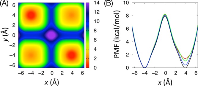
(A) Potential energy, U(x,y), of the model system with H_y = 6 in eq 16. (B) The one-dimensional PMF, , calculated from U(x,y) (black) and the results of 120-ns simulation data from USMD (red), WEUSMD (green), and aWEUSMD (blue) with N = 31 windows. from U(x,y) is calculated by eq 1 and those from simulations are calculated by WHAM.

By varying H_y from 5 to 6.5 with the increment of 0.5, we performed 120-ns Langevin dynamics MD simulations of USMD, WEUSMD, and aWEUSMD for a set of the number of windows, N ∈ {21,31,41,51,61}, with two fixed end points at x_min = −6 Å and x_max = 6 Å. Initially, the windows were equally distributed along x with d = (x_max – x_min)/(N – 1) and k was obtained from eq 2. We have performed nine simulations for each set of H_y and N, where the initial x-coordinate was set to each window center. The initial y-coordinate y₀ was set to y₀ = 3.8 + 0.05r, where r ∈ {0,1,···,8}.

For a more realistic (and complicated) example, we considered the assembly of the right-handed GpA-TM dimer because it has been extensively studied for transmembrane (TM) helix assembly³²⁻³⁵ and represents one of the tightest interfacial packing (with the well-known GxxxG motif) among all the known TM helix interfaces. Such tight packing makes it challenging to sample the conformational space (e.g., right-handed to left-handed dimer at short helix−helix distance r_HH) and thus makes the GpA-TM to be a valuable target to assess the sampling power.³⁵ We defined the GpA-TM as ⁷²EITLI IFGVM AGVIG TILLI SYGIR⁹⁶, in which we have chosen C_α atoms of residues 76–92 to define the helix principal axis for r_HH and the crossing angle Ω.^36,37 For the NMR structure (PDB: 1AFO),³⁸ the calculated r_HH and Ω are 6.59 Å and −39.2°, respectively.³⁹ To test and compare the sampling power of WEUSMD and aWEUSMD, we prepared three sets of initial configurations of GpA-TM: left-handed (IS1, Ω < 0), right-handed (IS2, Ω > 0), and parallel (IS3, Ω ≈ 0) helix–dimer interfaces.

The initial configurations were generated from the NMR structure by translating each helix along r_HH and then by rotating the helices along the helix–helix distance vector for a desired Ω. A total of 80 windows were generated for each initial configuration set in a r_HH range 5.2–21 Å with d = Δr_HH = 0.2 Å and the restraint force constant k obtained from eq 2 for WEUSMD (initial k for aWEUSMD). Then, we have performed 200-ns WEUSMD and aWEUSMD for IS1, IS2, and IS3. For computational efficiency, the IMM1 implicit membrane model⁴⁰ was used with the hydrophobic thickness of 23 Å to mimic a dimyristoylphosphatidylcholine (DMPC) lipid bilayer.

All the simulations were performed using CHARMM.⁴¹ For GpA-TM simulations, we used the SHAKE algorithm and default IMM1 options. We used a time step of 2 fs and the collision frequency γ = 5 ps^–1, which is a typical value for Langevin dynamics with proteins. Window exchanges were attempted every 1 ps and controlled by the REPDSTR module⁴² in CHARMM. In aWEUSMD, the window parameters were updated every 0.2 ns. The adaptive update were controlled by in-house Python scripts, which take the window parameters and the time series of ξ (x or r_HH) for all the windows from the previous simulation as input. The derivatives of the PMF ( and ) were calculated, for the numerical stability, using the cubic spline interpolation of obtained by the umbrella integration method.³¹ The resulting derivatives were used to obtain the updated window parameters for the next simulation by eqs 7 and 12–15. We limited the maximum shift of ξ_i in one update cycle by d/4 for its smooth evolution.

Results and Discussion

Toy Model

In this section, we show the results from a representative parameter set, H_y = 6 and N = 31 (see Supporting Information section S1 for the results from all the tested parameter sets). The one-dimensional (1D) PMF, , calculated from the results of USMD, WEUSMD, and aWEUSMD for y₀ = 4.1 are shown in Figure 2B. The accuracy of the aWEUSMD-PMF is the best among the three methods, while the WEUSMD-PMF is marginally better than the USMD-PMF. The most obvious reason for the improved accuracy of the PMFs from WEUSMD and aWEUSMD over USMD is the regular window exchange attempts, which facilitates the sampling of configurations. This improvement is clearly shown in Figure 3 by comparing the conditional probability, P(y|x) ≡ P(x,y)/P(x), where P(x) and P(x,y) are the populations sampled by simulations.

Figure 3.

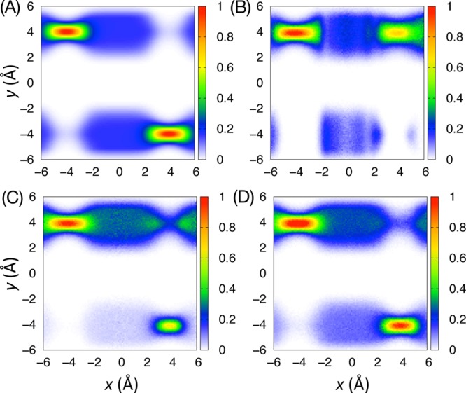
Conditional probability, P(y|x), calculated from (A) U(x,y), (B) USMD, (C) WEUSMD, and (D) aWEUSMD for H_y = 6 and N = 31. P(y|x) is normalized by max{P(y|x)|| x| ≤ 6 and |y| ≤ 6} and the binwidth is 0.1 Å for both x- and y-directions.

The sampling power (i.e., the accuracy of the sampling compared to the reference) can be quantitively estimated by the Kullback–Leibler divergence⁴³

18

where P_r(y|x) is calculated from U(x,y), N_bin,x is the number of bin size along x, and x_i and y_j are the i- and j-th bins along x and y, respectively. Smaller values of D_KL indicate better agreement of P(y|x) with P_r(y|x), and D_KL vanishes when they are identical. In addition, the relaxation time of D_KL, τ, can be a measure of the efficiency, estimated by fitting D_KL(t) to an exponential function: D_KL(t) = a+b exp (−t/τ). As shown in Figure 4A, the WEUSMD-D_KL (τ = 18.6 ± 1.1 ns) decays much faster than USMD-D_KL (τ = 68.5 ± 14.4 ns), and aWEUSMD-D_KL (τ = 8.91 ± 0.47 ns) relaxes even faster; similar results are obtained for most parameter sets examined (Supporting Information Figure S1 and Table S1).

Figure 4.

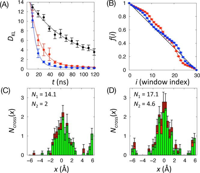
(A) Kullback–Leibler divergence D_KL calculated from 10-ns blocks of P(y|x) from USMD (black), WEUSMD (red), and aWEUSMD (blue) by eq 18. Shown together are the exponential fits of D_KL (dashed lines). (B) The fraction of replicas that have visited the lowest-index window, f(i), in eq 19, from WEUSMD (red) and aWEUSMD (blue) simulations. Shown together is f(i) for the ideal random walk of replicas (black line). (C–D) The histogram of the number of y-barrier crossing, N_cross(x), from (C) WEUSMD and (D) aWEUSMD simulations. N_cross(x) is the sum of the number of crossing from y > 0 to y < 0, N₁(x) (green), and that in the opposite direction, N₂(x) (red). The total number of y-barrier crossing is denoted by N_cross and similarly by N₁ and N₂. In all the figures, the data are averaged over nine independent simulations and the error bars represent the standard errors.

The efficiency gain in aWEUSMD over WEUSMD can be attributed to the optimal window distribution (P_a = 0.4) with k^eff(x), where the windows are concentrated in steep PMF (high ) regions. In these regions, the y-barrier is lower than those around 1D-PMF minima (x = 4 or −4 in Figure 2B), which results in better sampling along y-direction in aWEUSMD, that is, the increased number of y-barrier crossing N_cross (Figures 4C and D). As expected, there is no meaningful increase in N_cross from WEUSMD compared to that from USMD (Supporting Information Figure S2 and Table S2). Considering the fact that aWEUSMD optimizes WEUSMD only along the explicit CV (i.e., the x axis), the increase in N_cross (along the y axis) is noteworthy.

In addition, there is an efficiency gain from the improved random walk of replicas, which can be quantified as the fraction of replicas that have visited the lowest-index window most recently,^11,44

19

where n₀(i) is the accumulated number of replicas with traveling state “0” monitored at window i during the course of simulation and n_N–1(i) is similarly defined. The traveling state of a given replica is assigned (or updated) to “0” or “N – 1” only when it reaches at the lowest- or the highest-index window, 0 or N – 1, respectively. For the ideal random walk of replicas, f(i) should be linear.^11,44 By comparing eq 3 with eq 25 in ref (45) (a work for the optimization of replica’s random walk), it is clear that aWEUSMD indeed improves the random walk as well, as shown in Figure 4B; similar results are obtained for most parameter sets examined (Supporting Information Figure S3).

GpA-TM Assembly

In this section, we show the results from the WEUSMD and aWEUSMD for the assembly of the GpA-TM starting with the initial configurations with left-handed (IS1) and right helix–dimer interfaces (IS2) (see Supporting Information section S2.2 for the results from the parallel TM dimer initial configurations, IS3). Figure 5 shows the 1D-PMF as a function of r_HH, (r_HH), for IS1 and IS2. There is significant difference between the IS1-PMF and the IS2-PMF from WEUSMD, which is originated from incomplete sampling (see Figures 6A and C). The agreement between the IS1-PMF and the IS2-PMF from aWEUSMD is significantly improved, which we attribute to the improved sampling power of aWEUSMD over WEUSMD.

Figure 5.

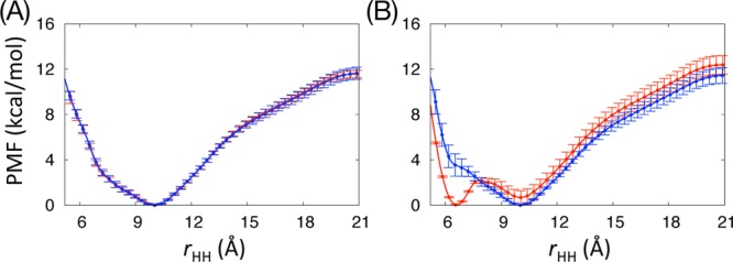
PMF as a function of r_HH, (r_HH), calculated from WEUSMD (red) and aWEUSMD (blue) starting from the initial configurations of (A) left-handed (IS1) and (B) right-hand (IS2) helix-dimer interfaces. For the PMF calculation, we used trajectories from 40 ns to 200 ns. The error bars represent the standard deviations calculated from 16 10-ns block average PMFs.

Figure 6.

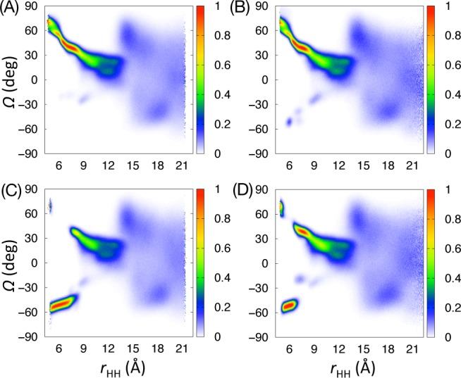
Conditional probability, P(Ω|r_HH), calculated from the results of (A) WEUSMD and (B) aWEUSMD for IS1. P(Ω|r_HH) calculated from the results of (C) WEUSMD and (D) aWEUSMD for IS2. P(Ω|r_HH) is normalized by max{P(Ω|r_HH)} and the binwidth is Δr_HH = 0.05 Å and ΔΩ = 6°.

The improved sampling efficiency of aWEUSMD over WEUSMD is supported by the conditional probability P(Ω|r_HH), as shown in Figure 6. The agreement between P(Ω|r_HH) calculated from aWEUSMD for IS1 and IS2 is improved up to shorter r_HH ≈ 7 Å (Figures 6B and 6D) compared to the results from WEUSMD, which show good agreement for r_HH > 9 Å. This improvement allows the sampling of the right-handed NMR structure-like conformations in aWEUSMD with IS1 (Figure 6B and Supporting Information Figure S4B), indicating that aWEUSMD indeed promotes the sampling along Ω, where no restraint potential was applied.

The sampling power of aWEUSMD and WEUSMD for the GpA-TM assembly are quantitatively compared by D_KL of P_t(Ω|r_HH) with respect to P_r(Ω|r_HH) from the results of 2D-WEUSMD in our previous work,³⁵ where P_t(Ω|r_HH) is calculated from the trajectories up to time t. As shown in Figure 7, the aWEUSMD-D_KL relaxes faster to its estimated steady-state value, D_KL^ss, compared to the WEUSMD-D_KL. For IS1, the estimates of (D_KL,τ) from aWEUSMD and WEUSMD are (0.515 ± 0.004,10.27 ± 0.53 ns) and (1.538 ± 0.002,14.20 ± 0.76 ns), respectively. For IS2, these estimates are (0.185 ± 0.003,12.84 ± 0.89 ns) and (0.541 ± 0.021,37.89 ± 3.59 ns) for aWEUSMD and WEUSMD, respectively. Although D_KL is a quantity that dictates both the accuracy and the efficiency of the sampling, it should be noted that this quantity is not always available in general because the probability distribution of the reference state needs to be known a prior.

Figure 7.

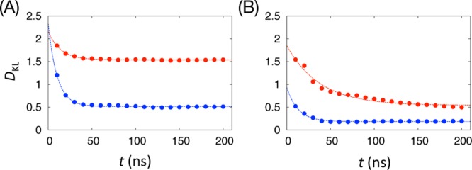
Kullback–Leibler divergence D_KL calculated using P_t(Ω|r_HH) from WEUSMD (red) and aWEUSMD (blue) for (A) IS1 and (B) IS2 by eq 18 with respect to P_r(Ω|r_HH) calculated from 2D-PMF in ref (35). P_t(Ω|r_HH) is calculated from trajectories up to time t. Shown together are the exponential fits of D_KL (dashed lines).

In aWEUSMD, as shown in Figure 8, the window parameters relax to their limiting values once the PMF is converged (albeit with fluctuations). The relaxation time of the window centers (including the effective ones) was estimated to be about 4 ns (20 update cycles). The estimated τ of the bias force constants (including the effective ones) are about 20 ns and 26.5 ns for IS1 and IS2, respectively. Interestingly, τ for the bias force constants are well correlated to that of D_KL. This good correlation enables us to estimate the efficiency by τ of window parameters without the need of D_KL. However, it should be noted that the converged window parameters does not guarantee the convergence of the PMF to the true one because aWEUSMD does not actively sample along the hidden DOF.

Figure 8.

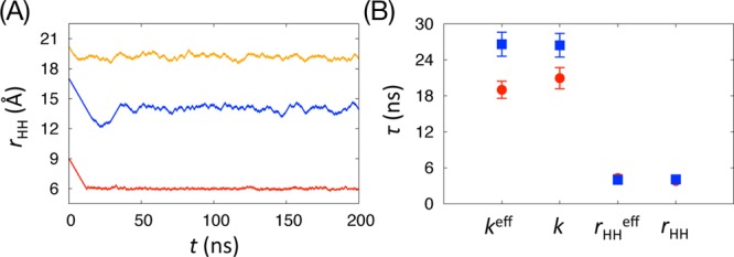
(A) Time-series of windows center (r_HH,i) for three windows (i = 19,59, and 75). (B) The average relaxation time τ of window parameters for IS1 (red) and IS2 (blue). The error bars are the standard errors of the average τ over the entire windows.

Discussion

Such an overlap problem can be alleviated in the present optimization method because of (1) the minimization of the shift in the windows center by the adaptively optimized (PMF-dependent) bias force constants and (2) the concentrated window distribution in the steep PMF regions with well-controlled overlap between neighboring windows by constraining P_a. However, it should be noted that, when N ≪ N_opt (ρ ≫ 1), aWEUSMD with fixed N cannot overcome this problem although it performs better than WEUSMD and USMD (data not shown). By relaxing the fixed N condition, aWEUSMD would be free of the overlap problem along ξ.

In this work, the efficiency of all the tested methods (USMD, WEUSMD, and aWEUSMD) was estimated by the relaxation time (τ) of D_KL. We observed that τ of D_KL is well correlated with that of window parameters which would be stable once the PMF is converged. Therefore, even in a situation in which one cannot calculate D_KL because of unknown reference state, the sampling efficiency (especially, convergence rate) can be estimated by τ of the window parameters (see Figure 8).

As shown in Figure 4A, the efficiency and sampling power of aWEUSMD and WEUSMD are significantly better than those of USMD due to the REX. The quality of REX is improved by aWEUSMD compared to that in WEUSMD, which is more clearly shown for smaller N but becomes less obvious as N increases (Figure S3). In Figure 9, we plotted f(i) obtained from the results of WEUSMD and aWEUSMD for the GpA-TM assembly. Although the quality of REX was improved by aWEUSMD, the significant nonlinearity in f(i) indicates that aWEUSMD has limited power in optimization of the flux of replicas, which we attribute to the incomplete sampling along the hidden DOF due to high barriers (>6 kcal/mol).

Figure 9.

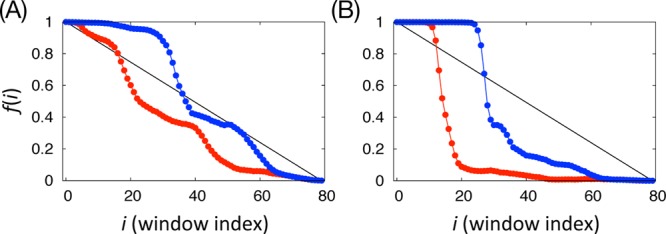
Fraction of replicas that have visited the lowest-index window, f(i), in eq 19, from WEUSMD (red) and aWEUSMD (blue) simulations for (A) IS1 and (B) IS2. Shown together is f(i) for the ideal random walk of replicas (black line).

The REX itself does not improve the barrier crossing along the hidden DOF for a given replica (see Supporting Information Figure S2). However, in aWEUSMD, where the windows are more densely distributed in the steep PMF regions (with optimal bias force constants), there are more barrier crossing events than WEUSMD and USMD. This implies that the present adaptive optimization method indeed improves the sampling efficiency of US along the hidden DOF. However, it should be noted that aWEUSMD does not actively sample the hidden DOF, as attempted in some recent efforts.^28,29 Therefore, the efficiency gain in aWEUSMD over WEUSMD is limited by the barrier height along the hidden DOF. The results from the toy-model suggests that aWEUSMD can overcome the barriers along the hidden DOF, whose height is up to about 6 kcal/mol. It is consistent with the results from the GpA-TM assembly in that the sampling along Ω is improved up to r_HH ≈ 7 Å, at which the barrier height along Ω is about 6 kcal/mol.³⁵

Concluding Remarks

In this work, we present a theory of adaptive optimization for umbrella sampling for optimal PMF calculations based on two constraints: (1) the uniform thermodynamic length for all the windows () and (2) the uniform average acceptance probability between neighboring windows (P_a = 0.4). From the first constraint, we obtained an analytic expression for the effective bias force constant k^eff(ξ). Then, the windows are distributed by constraining P_a = 0.4, which is known to be optimal for the exchange scheme chosen for the present work.

As an immediate consequence of the present theory, an estimate of the optimal number of windows N_opt and a parameter ρ (=N_opt/N) are obtained. The latter provides a criterion from which one can judge whether the given number of windows N is sufficient or not: when ρ ≈ 1, N is close to N_opt. Sampling along ξ by aWEUSMD would be proper as long as ρ ≤ 1, whose efficiency can be conveniently estimated by the relaxation time (τ) of the window parameters. However, when N ≪ N_opt, aWEUSMD with fixed N cannot overcome the overlap problem, which is an intrinsic limitation of any US-type methods. By relaxing the fixed N condition, aWEUSMD would be free of the overlap problem along ξ.

The efficiency gain in aWEUSMD over WEUSMD originates from the optimal window distribution concentrated in the steep PMF regions, where more barrier crossing along the hidden (or orthogonal) DOF are feasible, and also from the consequently improved random walk of replicas. As a result, the synergetic improvements in the sampling along both explicit and hidden DOF by aWEUSMD make the PMF converge faster than WEUSMD. However, it should be noted that the advantage of aWEUSMD over WEUSMD is limited by the barrier height along the hidden DOF. The results from the two test cases suggest that aWEUSMD can help sampling along the hidden DOF, whose barrier height is up to about 6 kcal/mol.

In this work, we fixed N in aWEUSMD for comparison with USMD and WEUSMD with the same N. If we relax this condition, a better performance of aWEUSMD would be achieved by employing self-learning scheme, analogous to that in the self-learning adaptive US.⁵ In this scheme, windows are added gradually until N reaches N_opt starting from aWEUSMD with small N. Then, aWEUSMD would be free of the overlap problem and would exploit its other advantages over WEUSMD (improved random walk of windows and sampling along the hidden DOF) simultaneously. This version of aWEUSMD (self-learning aWEUSMD) would be more useful in one-dimensional US simulations for efficient sampling and PMF calculations.

Glossary

Abbreviations

PMF

potential of mean force

CV

collective variable

MD

molecular dynamics

MC

Monte Carlo

US

umbrella sampling

REX

replica exchange

DOF

degrees of freedom

WEUS

window exchange US

aWEUSMD

adaptive WEUSMD

Appendix: An Accurate Analytic Expression for P_a

Here, we derive an accurate analytical approximate expression for P_a between a pair of windows i and j for arbitrary window parameters (ξ_i,k_i) and (ξ_j,k_j), whose corresponding effective window parameters, (ξ_i^eff, k_i) and (ξ_j^eff, k_j). Formally, P_a between the pair of windows is given by the integral,

20

where subscripts 1 and 2 are indices for a pair of windows i and j, P_ex = min{1,exp(−βΔ)} is the metropolis criterion for the exchange between the pair, and Δ is

21

It can be shown easily that

22

Simply, one can evaluate P_a by the numerical integration of eq 13 (or eq 22). However, its analytical expression can provide deeper understanding and insights, which is helpful in further applications. For example, when k_i^eff = k_j, the exact analytical expression of eq 13 is available,⁹ which is utilized to obtain eq 2 for the relationship between the window force constant and the window spacing for WEUSMD. In general cases (when k_i^eff ≠ k_j), there has been no such analytical expression for P_a, which we are in need of, for fast and accurate evaluation of eq 13 in order to redistribute windows in our adaptive optimization for US method.

The starting point is rewriting eq 13 in a symmetric form as

23

where, for m ∈ {i,j}, the kernels in eq 23 are defined as

24

and erf(x) is the error function of x, f_m = z_m²/(z_i – z_j²), z_m ≡ |Δξ_j,i|/(√2σ_m), Δξ_j,i^eff ≡ |ξ_j – ξ_i^eff|, and σ_m = (βk_m)^−1/2. Hereafter, we assume that k_j^eff > k_i (z_i > z_j). When k_j^eff < k_i, one can use the result after exchanging indices i and j.

To make eq 23 be integrable, we introduced a Gaussian approximation of the error function,

25

where sign(x) is the sign function of x. With 100 000 equally distributed supporting points along x in a range of [1.0 × 10^–20,5.0], the coefficients c₁ and c₂ are determined from the numerical fit to log[1–erf(x)] = 2c₁x + c₂x² as c₁ = −0.425672 and c₂ = −0.913347, respectively. After substitution of eqs 24 and 25 into eq 23, the integrals become those of Gaussian, whose analytic solution is available⁴⁶

26

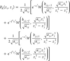
Using eq 26, we obtained an analytic approximate expression for P_a as a function of z₁ and z₂,

27

where

28a

28b

28c

28d

Here, erfc(x) = 1–erf(x) is the complementary error function, Ω(x) = exp(x²)erfc(x), W(x,y) = exp(x²)erfc(x + y), f = f_i + f_j, and a_m,n = 1 – c₂(z_m/z_n)² and b_m,n,r = rz_m – c₁(z_n/z_m) for m ∈ {i, j} and n ∈ {i,j} (m ≠ n).

We compared the exact expression for P_a for k_i^eff = k_j (z_i = z_j ≡ z), eq 4 in ref (9), with the equal z limit of eq 27 obtained by taking limit z_i → z and z_j → z,

29

As shown in Figure 10A, eq 29 agrees excellently with the exact solution. The absolute error is less than 1.48% (at z = 0.856) for any z ≥ 0 and the relative error is less than 8.94% (at z = 2.459) for z ∈ [0,6], which verified the accuracy of eq 27. In Figure 10B, eq 27 as a function of z₁ and z₂, P_a(z₁,z₂), is shown, in which the green area is the region of the interest (P_a ∼ 0.4) for the optimal overlap between neighboring windows.

Figure 10.

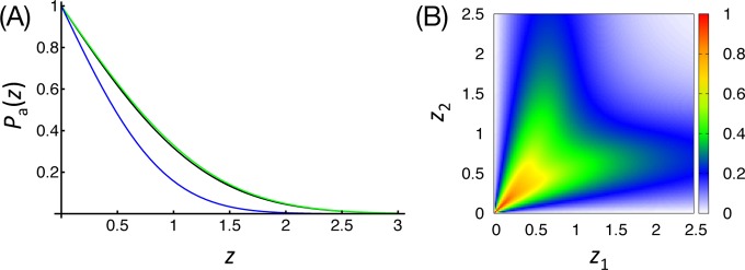
(A) The average acceptance probability, P_a(z), calculated from the exact solution, eq 4 in ref (9). (black), and the equal z limit of eq 27, eq 29 (green). Shown together is erfc(z) (blue), which is the first term of the approximate expression of P_a given by eq 29. (B) The average acceptance probability as a function of z₁ and z₂, P_a(z₁,z₂), given by eq 27.

Supporting Information Available

S1: Data for the toy model from all the tested parameter sets. S2: Additional data for the GpA-TM assembly. This material is available free of charge via the Internet at http://pubs.acs.org/.

The authors declare no competing financial interest.

Funding Statement

National Institutes of Health, United States

References

- Torrie G. M.; Valleau J. P. J. Comput. Phys. 1977, 23, 187–199. [Google Scholar]
- Mezei M. J. Comput. Phys. 1987, 68, 237–248. [Google Scholar]
- Marsili S.; Barducci A.; Chelli R.; Procacci P.; Schettino V. J. Phys. Chem. B 2006, 110, 14011–14013. [DOI] [PubMed] [Google Scholar]
- Maragakis P.; van der Vaart A.; Karplus M. J. Phys. Chem. B 2009, 113, 4664–4673. [DOI] [PMC free article] [PubMed] [Google Scholar]
- Wojtas-Niziurski W.; Meng Y.; Roux B.; Berneche S. J. Chem. Theory Comput. 2013, 9, 1885–1895. [DOI] [PMC free article] [PubMed] [Google Scholar]
- Kumar S.; Bouzida D.; Swendsen R. H.; Kollman P. A.; Rosenberg J. M. J. Comput. Chem. 1992, 13, 1011–1021. [Google Scholar]
- Vaneerden J.; Briels W. J.; Harkema S.; Feil D. Chem. Phys. Lett. 1989, 164, 370–376. [Google Scholar]
- Lee J.; Im W. Phys. Rev. Lett. 2008, 100, 018103. [DOI] [PubMed] [Google Scholar]
- Park S.; Kim T.; Im W. Phys. Rev. Lett. 2012, 108, 108102. [DOI] [PMC free article] [PubMed] [Google Scholar]
- Lingenheil M.; Denschlag R.; Mathias G.; Tavan P. Chem. Phys. Lett. 2009, 478, 80–84. [DOI] [PubMed] [Google Scholar]
- Nadler W.; Hansmann U. H. E. Phys. Rev. E 2007, 75, 026109. [DOI] [PubMed] [Google Scholar]
- Kofke D. J. Chem. Phys. 2002, 117, 6911–6914. [Google Scholar]
- Predescu C.; Predescu M.; Ciobanu C. J. Phys. Chem. B 2005, 109, 4189–4196. [DOI] [PubMed] [Google Scholar]
- Dashti D. S.; Roitberg A. E. J. Chem. Theory Comput. 2013, 9, 4692–4699. [DOI] [PubMed] [Google Scholar]
- Crooks G. E. Phys. Rev. Lett. 2007, 99, 100602. [DOI] [PubMed] [Google Scholar]
- Shenfeld D. K.; Xu H.; Eastwood M. P.; Dror R. O.; Shaw D. E. Phys. Rev. E 2009, 80, 046705. [DOI] [PubMed] [Google Scholar]
- Weinhold F. J. Chem. Phys. 1975, 63, 2479–2483. [Google Scholar]
- Salamon P.; Berry R. S. Phys. Rev. Lett. 1983, 51, 1127–1130. [Google Scholar]
- Salamon P.; Nulton J. Europhys. Lett. 1998, 42, 571–576. [Google Scholar]
- Schaller M.; Hoffmann K.; Siragusa G.; Salamon P.; Andresen B. Comput. Chem. Eng. 2001, 25, 1537–1548. [Google Scholar]
- Nulton J.; Salamon P. J. Non-Equilib. Thermodyn. 2002, 27, 271–288. [Google Scholar]
- Bennett C. J. Comput. Phys. 1976, 22, 245–268. [Google Scholar]
- Shirts M.; Bair E.; Hooker G.; Pande V. Phys. Rev. Lett. 2003, 91, 140601. [DOI] [PubMed] [Google Scholar]
- Maragakis P.; Spichty M.; Karplus M. Phys. Rev. Lett. 2006, 96, 100602. [DOI] [PubMed] [Google Scholar]
- Sugita Y.; Okamoto Y. Chem. Phys. Lett. 1999, 314, 141–151. [Google Scholar]
- Sugita Y.; Kitao A.; Okamoto Y. J. Chem. Phys. 2000, 113, 6042–6051. [Google Scholar]
- Darve E.; Rodriguez-Gomez D.; Pohorille A. J. Chem. Phys. 2008, 128, 144120. [DOI] [PubMed] [Google Scholar]
- Zheng L.; Chen M.; Yang W. Proc. Natl. Acad. Sci. U.S.A. 2008, 105, 20227–20232. [DOI] [PMC free article] [PubMed] [Google Scholar]
- Zheng L.; Chen M.; Yang W. J. Chem. Phys. 2009, 130, 234105. [DOI] [PubMed] [Google Scholar]
- Laio A.; Parrinello M. Proc. Natl. Acad. Sci. U.S.A. 2002, 99, 12562–12566. [DOI] [PMC free article] [PubMed] [Google Scholar]
- Kästner J.; Thiel W. J. Chem. Phys. 2005, 123, 144104. [DOI] [PubMed] [Google Scholar]
- Hènin J.; Pohorille A.; Chipot C. J. Am. Chem. Soc. 2005, 127, 8478–8484. [DOI] [PubMed] [Google Scholar]
- Zhang J.; Lazaridis T. Biophys. J. 2006, 91, 1710–1723. [DOI] [PMC free article] [PubMed] [Google Scholar]
- Li P.-C.; Miyashita N.; Im W.; Ishido S.; Sugita Y. J. Comput. Chem. 2014, 35, 300–308. [DOI] [PMC free article] [PubMed] [Google Scholar]
- Park S.; Im W. J. Chem. Theory Comput. 2013, 9, 13–17. [DOI] [PMC free article] [PubMed] [Google Scholar]
- Im W.; Lee J.; Kim T.; Rui H. J. Comput. Chem. 2009, 30, 1622–1633. [DOI] [PubMed] [Google Scholar]
- Lee J.; Im W. J. Comput. Chem. 2007, 28, 669–680. [DOI] [PubMed] [Google Scholar]
- MacKenzie K.; Prestegard J.; Engelman D. Science 1997, 276, 131–133. [DOI] [PubMed] [Google Scholar]
- Chothia C.; Levitt M.; Richardson D. J. Mol. Biol. 1981, 145, 215–250. [DOI] [PubMed] [Google Scholar]
- Lazaridis T. Proteins 2003, 52, 176–192. [DOI] [PubMed] [Google Scholar]
- Brooks B. R.; Brooks C. L. III; Mackerell A. D. Jr.; Nilsson L.; Petrella R. J.; Roux B.; Won Y.; Archontis G.; Bartels C.; Boresch S.; Caflisch A.; Caves L.; Cui Q.; Dinner A. R.; Feig M.; Fischer S.; Gao J.; Hodoscek M.; Im W.; Kuczera K.; Lazaridis T.; Ma J.; Ovchinnikov V.; Paci E.; Pastor R. W.; Post C. B.; Pu J. Z.; Schaefer M.; Tidor B.; Venable R. M.; Woodcock H. L.; Wu X.; Yang W.; York D. M.; Karplus M. J. Comput. Chem. 2009, 30, 1545–1614. [DOI] [PMC free article] [PubMed] [Google Scholar]
- Woodcock H. L. III; Hodoscek M.; Gilbert A. T. B.; Gill P. M. W.; Schaefer H. F. III; Brooks B. R. J. Comput. Chem. 2007, 28, 1485–1502. [DOI] [PubMed] [Google Scholar]
- Kullback S.; Leibler R. A. Ann. Math. Statist. 1951, 22, 79–86. [Google Scholar]
- Trebst S.; Huse D. A.; Troyer M. Phys. Rev. E 2004, 70, 046701. [DOI] [PubMed] [Google Scholar]
- Escobedo F. A.; Martinez-Veracoechea F. J. J. Chem. Phys. 2007, 127, 174103. [DOI] [PubMed] [Google Scholar]
- Handbook of Mathematical Functioins With Formulas, Graphs, and Mathematical Tables; Abromowitz M., Stegun I. A., Eds.; Dover:: New York, 1972. [Google Scholar]
Associated Data
This section collects any data citations, data availability statements, or supplementary materials included in this article.