Multivariate Phase–Amplitude Cross-Frequency Coupling in Neurophysiological Signals

Abstract

Phase–amplitude cross-frequency coupling (CFC)—where the phase of a low-frequency signal modulates the amplitude or power of a high-frequency signal—is a topic of increasing interest in neuroscience. However, existing methods of assessing CFC are inherently bivariate and cannot estimate CFC between more than two signals at a time. Given the increase in multielectrode recordings, this is a strong limitation. Furthermore, the phase coupling between multiple low-frequency signals is likely to produce a high rate of false positives when CFC is evaluated using bivariate methods. Here, we present a novel method for estimating the statistical dependence between one high-frequency signal and N low-frequency signals, termed multivariate phase-coupling estimation (PCE). Compared to bivariate methods, the PCE produces sparser estimates of CFC and can distinguish between direct and indirect coupling between neurophysiological signals—critical for accurately estimating coupling within multiscale brain networks.

I. Introduction

There is increasing interest in clarifying the role of neuronal oscillations in shaping computation and communication in multiscale brain networks. The cognitive, systems, and computational neuroscience communities are investigating this topic for a number of reasons. First, neuronal oscillations or brain rhythms reflect rhythmic changes in cortical excitability [1]. Therefore, oscillations influence local computation since neuronal activity differs depending on its timing relative to the phase of ongoing oscillations. That is, stimulus processing may occur faster if stimuli are presented at the right time relative to ongoing oscillatory activity. Similarly, long-range communication may be influenced by the relative phase difference of oscillatory activity in different areas [2]. For example, the effective communication gain between two areas is maximized when there is an optimal phase difference between the signals arising from these areas, such that spikes leaving one area will arrive when the other area is maximally excitable. Furthermore, electrical brain activity is now commonly recorded at a variety of different spatial scales, from single-neuron spikes (action potentials) at the microscale to the EEG at the macroscale. These signals exhibit event-related changes in distinct frequency bands, such as the delta (1–4 Hz), theta (4–8 Hz), alpha (8–12 Hz), beta (12–30 Hz), and gamma (>30 Hz) bands. Different frequencies provide temporal windows for processing (corresponding to the duration of one oscillatory cycle) and coordinate groups of neurons over different spatial extent—low frequencies modulate activity over large spatial regions in long temporal windows, while high frequencies modulate activity over small spatial regions and short temporal windows [3]. Neuronal processing is distributed across multiple scales and may be regulated by a hierarchy of mutually interacting neuronal oscillations [4]. Transient interactions between different brain rhythms, termed cross-frequency coupling (CFC), can act as regulatory structures since different groups of neurons are coordinated by distinct frequencies. Of particular interest is the phase–amplitude CFC, which describes the dependence between the phase of a low-frequency (LF) brain rhythm and the amplitude (or power) of high-frequency (HF) activity (see Fig. 1). The phase–amplitude CFC has been observed in humans, macaques, and rats [3] and correlates with behavioral performance over the course of extended learning [5]. Thus, the phase–amplitude CFC is of interest to theorists because CFC provides one of the few physiologically plausible mechanisms able to coordinate fast, spike-based computation with the slower external and internal events that guide perception, action, and learning [3].

Fig. 1.

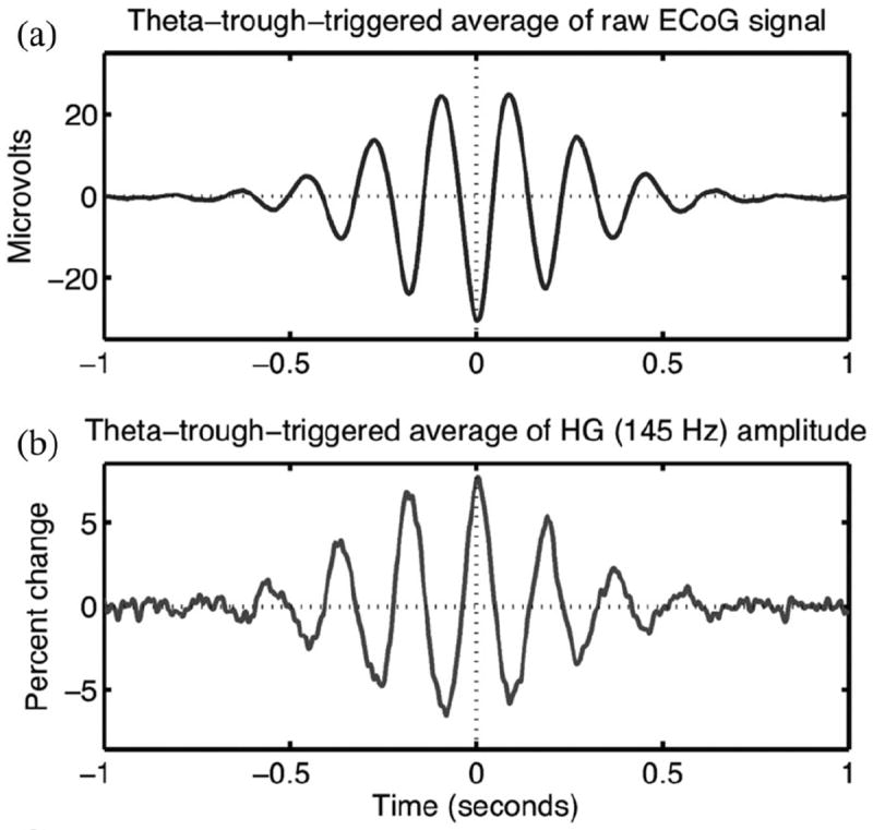
Example of phase–amplitude CFC in electrical activity recorded from human prefrontal cortex. (a) Averaging segments of the raw (unfiltered) electrocorticogram signal time locked to theta (6 Hz) troughs yields a transient theta oscillation. (b) Similar theta-trough-locked averaging of the high gamma (HG; 145 Hz) analytic amplitude reveals that HG amplitude undergoes fluctuations anticorrelated with the average waveform of the theta oscillation. Modulation of HF amplitude by LF phase is the defining feature of phase–amplitude CFC.

Several different analysis methods targeting the phase–amplitude CFC have been proposed [6], [7]. However, despite the increasing ease of multielectrode recordings, all of these CFC methods are inherently bivariate. That is, these methods investigate the relationship between activity in a LF and HF bands from one channel (within-channel CFC) or examine the dependence of HF activity (amplitude or power) of one channel upon the LF activity (phase) of another channel (cross-channel CFC). Here, we describe a novel method for assessing the statistical dependence of HF amplitude of one signal y upon a set of N LF phases from signals {x₁, x₂, …, x_N}. In the following, we first describe how to detect the phase–amplitude CFC using the bivariate phase-locking value (PLV) method and describe the relation of the PLV to the von Mises probability density function (pdf). Next, we describe the multivariate phase-coupling estimation (PCE) technique and apply it to a simple three-signal test case involving one HF signal and two LF signals. Even in this simple case, the bivariate PLV and multivariate PCE methods differ in their assessment of the statistical significance and strength of CFC—differences that have an important impact upon the inferred network structure.

II. Assessing Cross-Frequency Coupling via the Bivariate PLV

One of the more robust yet sensitive techniques for investigating CFC is the PLV method [6]. Importantly, this method is already familiar to neuroscientists who use it to estimate same-frequency, cross-channel phase coupling [8]. The same mathematical approach and statistical evaluation can be used to investigate single-channel, cross-frequency interactions once activity from both frequency bands is expressed in terms of phase variables. Specifically, given a (real-valued) raw signal x(t), we can filter it to produce two (complex-valued) signals: T_HF [x(t)] = x_HF (t) = A_HF (t) exp[iθ_HF (t)] (where $i=\sqrt{-1}$), reflecting HF activity, and T_LF [x(t)] = x_LF (t) = A_LF (t) exp[iθ_LF (t)], reflecting LF activity. The filter operator T_F [x(t)] can be implemented in a variety of mathematically equivalent ways [9]; here, we assume convolution with a complex-valued Gabor basis function with a Gaussian envelope. Band-pass filtering followed by the Hilbert transform is another common choice.

CFC techniques are designed to assess the relationship between the phase time series θ_LF (t) and amplitude time series A_HF (t), but the PLV method requires both signals to be expressed in terms of phase variables restricted to the interval [−π, π). This is true for θ_LF (t) but not for A_HF (t). Therefore, the PLV method applies a second filtering operation to extract the LF component of the HF amplitude time series: T_LF [|T_HF [x(t)]|] = T_LF [|x_HF (t)|] = T_LF [A_HF (t)] = A_HFA (t) exp[iθ_HFA (t)], where |x| is the modulus or the absolute value of x. This second-order filtering yields the time series θ_HFA (t), reflecting the phase of LF variations of the amplitude time series of the HF filtered signal x (see Fig. 2). From the phase time series θ_HFA (t) and the phase time series θ_LF (t), we can compute the actual PLV as ${\mathrm{PLV}}_{\mathrm{REAL}}=\frac{1}{N}|{\sum }_{k=1}^N\exp [i({\theta }_{\mathrm{HFA}}(k)-{\theta }_{\mathrm{LF}}(k))]|$, where N is the number of sample points (here we only consider cases, where N is large). PLV_REAL is restricted to the real interval (0,1], with 1 corresponding to perfect phase locking and values close to 0 corresponding to little or no phase locking.

Fig. 2.

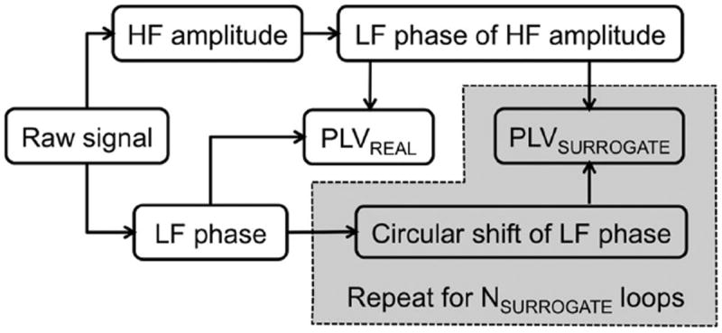
Analysis steps for the bivariate PLV method.

Finally, we can assess the statistical significance of PLV_REAL by comparing it to a set of surrogate (data-shuffled) PLVs {PLV_SURROGATE} (see Fig. 3). That is, for each (integer-valued) surrogate run s ∈ [1, 2, …, N_SURROGATE], compute PLV_S after randomly (circular) shifting one of the two time series. That is (with a slight abuse of notation), take the variable t to represent the ordered list of sample points: t = [t₁ :t_Ntime] = [t₁, t₂, …, t_Ntime]. Draw an integer K from the list [1:N_time] and then fix t_S = [t_K :t_Ntime, t₁: t_K−1]. Then θ_LF,S (t) = θ_LF (t_S), and ${\mathrm{PLV}}_S=\frac{1}{N}|{\sum }_{k=1}^N\exp [i({\theta }_{\mathrm{HFA}}(k)-{\theta }_{\mathrm{LF},S}(k))]$. If there are only M values in the set {PLV_SURROGATE } that are larger than PLV_REAL, then the one-tailed probability of PLV_REAL being due to chance is p = M/N_SURROGATE (if M = 0, fix p = 1/N_SURROGATE).

Fig. 3.

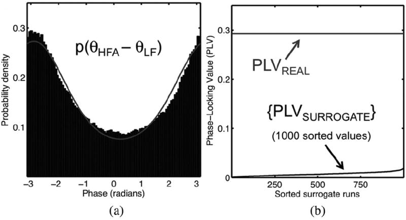
Example of CFC detection via the bivariate PLV method. The HF/LF bands are the same as the example in Fig. 1. (a) CFC manifests as the coupling between a LF phase variable (θ_LF) and a variable representing the LF phase component of the HF amplitude (θ_HFA). The distribution of phase differences θ_HFA – θ_LF (black histogram) is well fit by von Mises distribution (gray pdf); the more concentrated the distribution of phase differences θ_HFA – θ_LF, the larger the PLV. (b) Statistical significance of the PLV actually observed (PLV_REAL) can be assessed via a randomized permutation test that generates an ordered list of surrogate (data-shuffled) PLVs (see the text).

The PLV method is an excellent technique for estimating the strength and significance of instantaneous phase coupling between two brain signals, and it has been used to investigate a multitude of different functional brain networks [10]. Nonetheless, the PLV method suffers from two fundamental limitations that motivate the development of alternative methods. First, the output of the PLV method is a single scalar number or index rather than a probability distribution. This means that the PLV cannot be directly used to generate simulated data with identical phase-coupling characteristics. However, the set of relative phase differences used to calculate the PLV can also be used to fit a parametric pdf. One of the simplest and most tractable pdfs over circular or phase variables is the von Mises distribution: p(θ∣ϕ, γ) = exp[γ cos(θ − ϕ)]/2πI₀ (γ), where I_k (·) is the modified Bessel function of the kth order. The von Mises distribution is the simplest distribution possible given a phase angle ϕ and concentration parameter γ, in that the entropy of the distribution is maximized. The larger the value of γ, the more concentrated the distribution of phases will be around the angle ϕ. Once the von Mises parameters have been fit for a set of relative phase differences, then it is straightforward to generate synthetic data with the same phase-coupling properties as the empirically recorded data. Furthermore, there is a monotonic relationship between the PLV and the von Mises concentration parameter γ: PLV = I₁ (γ)/I₀ (γ) [2]. Each value of the PLV has a one-to-one mapping to a von Mises distribution with a given concentration (and vice versa), thus solving this first problem.

The second and more serious problem is that the PLV method is an inherently bivariate technique. That is, if N different local field potential (LFP) channels are simultaneously recorded during an experiment, the PLV method requires that all possible pairs of channels be examined separately, which can produce misleading results. For example, suppose we have a three-node network of coupled oscillators including nodes A, B, and C. If nodes A and B are both phase coupled to node C, then the phase value θ_A from node A and phase value θ_B from node B may nonetheless appear dependent even if there is no direct influence between nodes A and B. That is, it may be the case that p(θ_A, θ_B) ≠ p(θ_A) p(θ_B), but p(θ_A, θ_B∣θ_C) = p(θ_A∣θ_C) p(θ_B∣θ_C). Therefore, examining nodes A and B in isolation and ignoring the influence of node C may produce incorrect estimates of the network structure. The ideal case would be to fit a pdf describing the likelihood of seeing any possible N-dimensional vector of phases. In contrast to the PLV approach, such a multivariate pdf would permit sampling for simulations as well as avoiding issues of conditional dependence inherent in a highly interconnected network of coupled oscillators.

III. Assessing Cross-Frequency Coupling via the Multivariate PCE

In fact, such a multivariate phase distribution was derived recently [11]. Given an N-dimensional vector of phases, i.e., θ = (θ₁, θ₂, …, θ_N), extracted from N distinct signals, the maximum entropy distribution corresponding to the observed pairwise phase statistics is given as

$$p(\theta \mid \mathbf{K})=\frac{1}{Z(\mathbf{K})}\exp \left[\frac{1}{2}\sum _{m,n=1}^N{\kappa }_{\mathit{mn}}\cos ({\theta }_m-{\theta }_n-{\mu }_{\mathit{mn}})\right]$$ (1)

where the terms κ_mn and μ_mn are the coupling parameters between channels m and n. The Hermitian matrix K, with elements, i.e., K_mn = κ_mn exp[iμ_mn], specifies the parameters of the distribution, while the term Z(K) is the parameter-dependent normalization constant. An equivalent matrix–vector expression for the probability distribution is $p(\theta \mid \mathbf{K})=\frac{1}{Z(\mathbf{K})}\exp [\frac{1}{2}{\mathbf{Z}}^{†}\mathbf{Kz}]$, where z is an N-dimensional vector of unit-length complex variables, i.e., z_m = exp[iθ_m], and † represents the conjugate transpose. Each matrix element, i.e., K_mn = κ_mn exp[iμ_mn], encodes the coupling strength between channels m and n (as the modulus κ_mn) as well as the preferred phase offset between m and n (the angle μ_mn). The term κ representing coupling strength in the multivariate phase distribution is analogous to the concentration parameter γ in the von Mises distribution. The normalization constant Z(K) is a function of the coupling matrix and a general analytic formula for Z(K) has not yet been found [11]. However, an efficient technique based on score-matching can nonetheless be used to estimate distribution parameters from observed phase data [11]. MATLAB and Python code to estimate the distribution are available at [12]. We call this approach the multivariate PCE method.

The analysis flow of the multivariate PCE method is similar to the bivariate PLV approach, except that rather than inputing one HF signal and one LF signal, we now input one HF signal and N LF signals. Similarly, statistical significance of the estimated parameters can be assessed using the same permutation testing technique, by shifting the one HF signal relative to the N LF signals. Importantly, however, instead of producing a single parameter PLV_REAL or the pair of von Mises parameters (ϕ, γ), the PCE method produces an N × N parameter matrix K. The power of the multivariate PCE method is that it is able to separate (or distinguish) direct from indirect coupling. That is, the direct interaction between two oscillators m and n (n ↔ m) is captured by the matrix entry K_nm = κ_nm exp[iμ_nm], while indirect interactions (n ↔ k ↔ m, k ≠ {n, m}) are captured by the rest of the parameter matrix K.

Just as we can map PLV onto the von Mises pdf (capturing the distribution of phase differences due to both direct and indirect coupling), we can map K_mn onto a pdf representing the influence of direct coupling alone: p(θ_m − θ_n ∣ μ_mn, κ_mn) = exp[κ_mn cos(θ_m − θ_n − μ_mn)]/2πI₀ (κ_mn) [2]. We term this distribution the isolated distribution, since it is the distribution that would result if all indirect coupling were removed, isolating the two nodes of interest from the rest of the network. Critically, proper assessment of CFC requires us to estimate this direct coupling rather than the lumped coupling seen by the bivariate methods, as shown by the following example.

IV. Differences in CFC Estimates Obtained from the PLV and PCE Methods

Fig. 4 shows a simple case of multivariate CFC in electrocorticogram (ECoG) data recorded from human prefrontal cortex (6.1 min, 736 391 sample points) [13]. One ECoG channel was filtered at HF and LF (110 and 6 Hz, respectively) to generate HF and LF signals (HFA and LF1). A different ECoG signal was filtered at 6 Hz to generate the second LF signal (LF2). Critically, LF1 and LF2 are strongly phase coupled [see Fig. 4(a)], and as part of an indirect path, this LF phase coupling can influence the estimate of CFC. For example, while the distribution of θ_HFA − θ_LF1 is more concentrated than 1000 surrogate distributions, indicating strong CFC, the bivariate PLV and multivariate PCE methods differ on the assessment of CFC between HFA and LF2. While the distribution of θ_HFA − θ_LF2 is more concentrated than all 1000 surrogate distributions (see Fig. 4(c), black arrow)—and would therefore be considered significant by the PLV method at p ≤ 0.001—PCE can explain this concentration as being due to indirect coupling between HFA and LF2 via the intermediate node LF1. Therefore, while the bivariate PLV method (erroneously) finds the significant CFC between HFA and LF2, the multivariate PCE method does not. Importantly, while we used a simple three-node example here, the multivariate PCE method can be applied to any number of simultaneously recorded channels, as shown via simulations in [14].

Fig. 4.

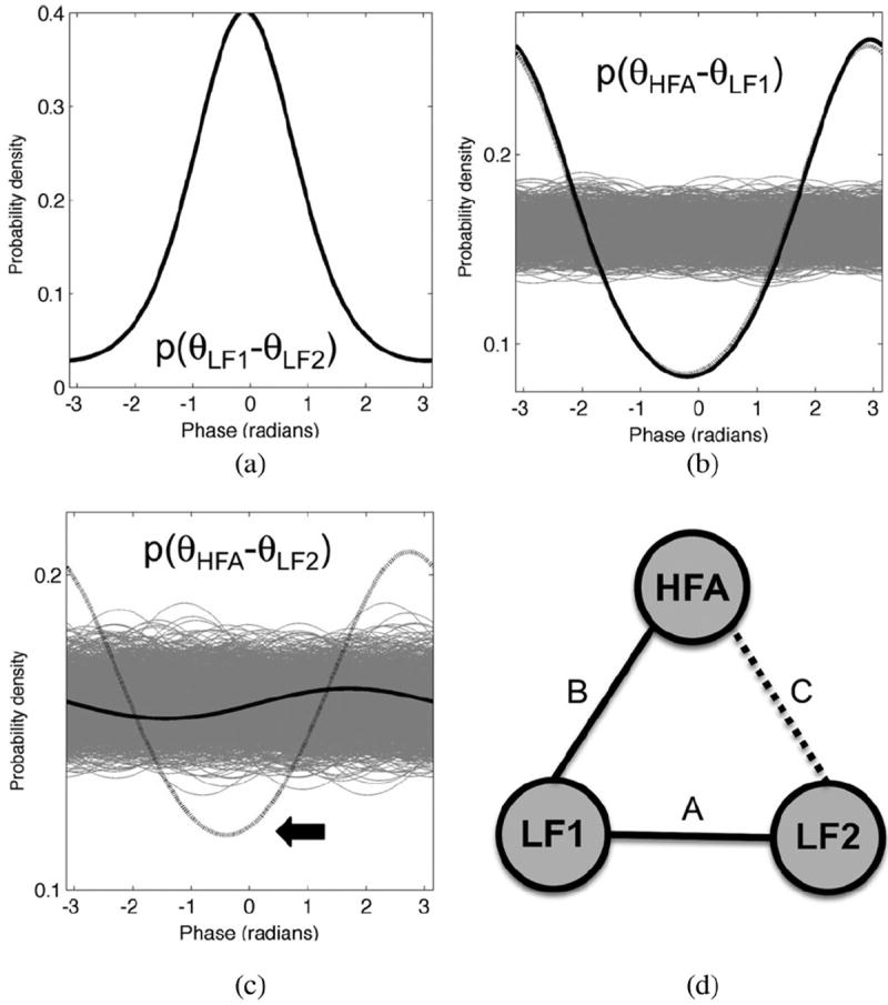
Example in which the PLV and PCE methods differ. θ_HFA and θ_LF1 are the same signals as in Fig. 3. θ_LF2 is the theta phase of a nearby (10 mm) electrode. (a) The distribution of theta phase differences θ_LF1 – θ_LF2 is strongly concentrated. (b) PLV and PCE estimates of CFC agree for nodes HFA and LF1, with the distributions of phase differences associated with the PLV (black, dotted) and PCE (black, solid) falling outside the range of all surrogate distributions (gray) generated via randomized permutation testing. (c) In contrast, PLV and PCE generate different estimates for the CFC between nodes HFA and LF2. The PLV method detects that the actual distribution of phase differences θ_HFA – θ_LF2 (dotted black line, see arrow) is outside the range of the surrogate distributions (gray), indicating that these nodes are indeed coupled. However, the PCE explains the coupling between HFA and LF2 via an indirect chain of coupling from LF2 to LF1 to HFA. The isolated distribution of θ_HFA – θ_LF2 (solid black line) represents the phase concentration due to direct coupling between HFA and LF2 alone. Since this isolated distribution falls within the range of surrogate distributions (gray), the CFC link between nodes HFA and LF2 is not statistically significant. (d) Schematic illustration of the three-node network that includes HFA, LF1, and LF2. Letters next to each link refer to the subpanel that shows the strength of coupling between nodes.

V. Conclusion

We have shown that the PCE approach is an effective method to assess multivariate phase–amplitude CFC in neurophysiological signals. Since this method employs the maximum entropy distribution that matches pairwise phase statistics [11], the PCE approach results in the most parsimonious coupling network that explains the observed data. The PCE method may produce erroneous results if there exist influential but unobserved (hidden) phase variables, but this is a concern for all currently employed methods. To our knowledge, the PCE approach is the first inherently multivariate method for estimating CFC. In summary, for a given set of N observed signals, the PCE is a natural extension of the PLV method to N dimensions [2], refines assessed coupling into direct and indirect influences [2], and results in sparser networks of coupling between signals [11].

References

- 1.Fries P. A mechanism for cognitive dynamics: neuronal communication through neuronal coherence. Trends Cogn Sci. 2005;9:414–410. doi: 10.1016/j.tics.2005.08.011. [DOI] [PubMed] [Google Scholar]
- 2.Canolty RT, Ganguly K, Kennerley SW, Cadieu CF, Koepsell K, Wallis JD, Carmena JM. Oscillatory phase coupling coordinates anatomically-dispersed functional cell assemblies. Proc Natl Acad Sci USA. 2010;107:17356–17361. doi: 10.1073/pnas.1008306107. [DOI] [PMC free article] [PubMed] [Google Scholar]
- 3.Canolty RT, Knight RT. The functional role of cross-frequency coupling. Trends Cogn Sci. 2010;11:506–514. doi: 10.1016/j.tics.2010.09.001. [DOI] [PMC free article] [PubMed] [Google Scholar]
- 4.Lakatos P, Shah AS, Knuth KH, Ulbert I, Karmos G, Schroeder CE. An oscillatory hierarchy controlling neuronal excitability and stimulus processing in the auditory cortex. J Neurophysiol. 2005;94:1904–1911. doi: 10.1152/jn.00263.2005. [DOI] [PubMed] [Google Scholar]
- 5.Tort ABL, Robert WK, Joseph RM, Nancy JK, Howard E. Theta-gamma coupling increases during the learning of item-context associations. Proc Natl Acad Sci USA. 2009;106:20942–20947. doi: 10.1073/pnas.0911331106. [DOI] [PMC free article] [PubMed] [Google Scholar]
- 6.Penny WD, Duzel E, Miller KJ, Ojemann JG. Testing for nested oscillation. J Neurosci Methods. 2008;174:50–61. doi: 10.1016/j.jneumeth.2008.06.035. [DOI] [PMC free article] [PubMed] [Google Scholar]
- 7.Tort ABL, Robert K, Howard E, Nancy K. Measuring phase–amplitude coupling between neuronal oscillations of different frequencies. J Neurophysiol. 2010;104:1195–1210. doi: 10.1152/jn.00106.2010. [DOI] [PMC free article] [PubMed] [Google Scholar]
- 8.Lachaux J-P, Rodriguez E, Martinerie J, Varela FJ. Measuring phase sychrony in brain signals. Human Brain Mapping. 1999;8:194–208. doi: 10.1002/(SICI)1097-0193(1999)8:4<194::AID-HBM4>3.0.CO;2-C. [DOI] [PMC free article] [PubMed] [Google Scholar]
- 9.Bruns A. Fourier-, Hilbert- and wavelet-based signal analysis: Are they really different approaches? J Neurosci Methods. 2004;137:321–332. doi: 10.1016/j.jneumeth.2004.03.002. [DOI] [PubMed] [Google Scholar]
- 10.Varela F, Lachaux J-P, Rodriguez E, Martinerie J. The brainweb: Phase synchronization and large-scale integration. Nat Rev Neurosci. 2001;2:229–239. doi: 10.1038/35067550. [DOI] [PubMed] [Google Scholar]
- 11.Cadieu CF, Koepsell K. Phase coupling estimation from multivariate phase statistics. Neural Comput. 2010;22:3107–3126. [Google Scholar]
- 12.(2010). [Online]. Available: https://github.com/koepsell/phase-coupling-estimation.
- 13.Canolty RT, Soltani M, Dalal SS, Edwards E, Dronkers NF, Nagarajan SS, Kirsch HE, Barbaro NM, Knight RT. Spatiotemporal dynamics of word processing in the human brain. Front Neurosci. 2007;1:185–196. doi: 10.3389/neuro.01.1.1.014.2007. [DOI] [PMC free article] [PubMed] [Google Scholar]
- 14.Cadieu CF, Koepsell K. A multivariate phase distribution and its estimation. 2008 Sep; arXiv:0809.4291v2 [q-bio.NC] [Google Scholar]