Multidimensional Texture Characterization: On Analysis for Brain Tumor Tissues Using MRS and MRI

Abstract

This paper investigates the efficacy of automated pattern recognition methods on magnetic resonance data with the objective of assisting radiologists in the clinical diagnosis of brain tissue tumors. In this paper, the sciences of magnetic resonance imaging (MRI) and magnetic resonance spectroscopy (MRS) are combined to improve the accuracy of the classifier, based on the multidimensional co-occurrence matrices to assess the detection of pathological tissues (tumor and edema), normal tissues (white matter — WM and gray matter — GM), and fluid (cerebrospinal fluid — CSF). The results show the ability of the classifier with iterative training to automatically and simultaneously recover tissue-specific spectral and structural patterns and achieve segmentation of tumor and edema and grading of high and low glioma tumor. Here, extreme learning machine – improved particle swarm optimization (ELM-IPSO) neural network classifier is trained with the feature descriptions in brain magnetic resonance (MR) spectra. This has the characteristics of varying the normal spectral pattern associated with tumor patterns along with imaging features. Validation was performed considering 35 clinical studies. The volumetric features extracted from the vectors of this matrix articulate some important elementary structures, which along with spectroscopic metabolite ratios discriminate the tumor grades and tissue classes. The quantitative 3D analysis reveals significant improvement in terms of global accuracy rate for automatic classification in brain tissues and discriminating pathological tumor tissue from structural healthy brain tissue.

Introduction

Brain tumors are complex in nature. A biology-based system research model can deliver more compelling insight. Brain tumors are the leading cause of solid tumor cancer death in children under the age of 20 [1]. Classification by combining multimodal proton MRS and morphological MR images of the brain in anatomic types of tissue from medical images is still a challenging task. Often, both anatomy and pathological diagnosis require intensive manual interaction for segmentation and classification.

Numerous studies in the early literatures have proposed different techniques towards classification of brain tumors based on diverse sources [2, 6, 22]. Amongst the most promising noninvasive methods in radiology towards diagnosis of brain tumors, magnetic resonance imaging (MRI) and magnetic resonance spectroscopy (MRS) are significant. MRI provides detailed soft tissue contrast information about brain tumor anatomy, cellular structure, and vascular supply, making it an important tool for the effective diagnosis, treatment, and monitoring of the disease. Anatomical structures and pathological structures like tumors or lesions have high diversity in sizes, shapes, locations, and intensities. An MRI sequence encloses information relevant to the tissue parameters. All image analysis and recognition models extract patterns with implied information and assist towards tissue characterization. MRS, a functional imaging technique that detects metabolic changes, is mainly used towards the study of tissue metabolism and for differentiating between tumor grades. The most significant biochemical signals provide useful information on brain tumor grades [14]. Leveraging towards other functional imaging techniques, MRS does not utilize high-energy radiation and contrast agents or labeled markers. Discrimination in types of tumor grade requires additional information. In contrast, metabolite spectra from the MRS imaging add new dimension towards discrimination of lesions [5]. Changes in the intensity of individual images are generally not sufficiently specific for diagnostics of tumors from MRI. Hence, different additional patterns across multiple resonances are required.

Need for a Multidimensional Texture Analysis for the Characterization of a Brain Tumor

Context of Contemporary Status

Limited work has been carried out in the area of characterization and analysis of 3D (volumetric) textures using MRI, MRS, and both MRI and MRS [5, 9, 10, 24, 25]. Dou et al. [27] proposed the glial tumor segmentation method using data fusion of MRI and MRS based on fuzzy-based method. A model to create nosologic images of the brain based on MRI and MRS imaging was developed. The abnormality, edema and tumor, was detected based on atlas, outlier detection, intensities, and application of geometric spatial constraints using least squares support vector machine (LS-SVM) [18]. An approach in combining both textural and spectroscopic features have achieved mean classification accuracy of 99 % for discriminating between low and high-grade tumors by Devos et al. [7]. Luts et al. combined four textural features and ten spectroscopic features, with LS-SVM classification algorithm towards discrimination of different tumor types with promising results [19]. A support vector machine (SVM)-based system was investigated on acquired postcontrast MR image and spectroscopic features improving discrimination between meningiomas and metastasis [28]. Georgiadis et al. proposed 3D gray-level co-occurrence matrix–run-length matrix (GLCM–RLM) with MRS features achieving 100 % accuracy using LSFT-SVM model [11]. However, the computational time required for the training and evaluation procedures was very high (approximately 11 h) which attributed to the iterative methods used for the best feature selection (exhaustive search) and for the system’s evaluation in the proposed classification system. Although the SVM classifier has been shown to provide a good generalization performance, results are often far from the theoretically expected level, because SVM implementation employs approximation techniques.

Need for a Volumetric Feature Extraction Design Model

Various grades of tumor do suggest primary tumor which involves radiological features and requires macroscopic appearance for further clinical analysis [19]. Earlier, quite a few studies have been proposed combining MR textural and spectroscopic analyses, to provide clinicians’ second opinion tools that will assist them in the characterization of brain tumors [28]. On the other hand, studies have relied on the 2D textural feature thus depriving their system from higher-order, information rich, textural features and involve more metabolites that are cumbersome to quantify on MRI in everyday clinical routine [28].

Similarly in Georgiadis et al. and Wang et al. [11, 28], a series of 3D textural features were extracted based on the volume-of-interest’s (VOI’s) histogram, volumetric co-occurrence matrices, and run-length matrices. Since the feature extraction methods cannot generate features that are all discriminative for classification, feature selection techniques have been increasingly used in MRI brain tissue classification. To achieve the best classification performance, the use of subset feature selection methods that generally have better performance is required. However, the rich high computational cost of subset feature selection methods limits their application to problems with high feature dimensionality as in previous studies [11, 29]. To leverage the advantages and overcome the limitations of the abovementioned feature extraction and selection techniques, an integrated feature extraction and selection method for neuroimage classification is proposed. The model for 3D texture analysis is based on extended multidimensional co-occurrence matrices.

Problem Definition

The major challenge towards fusion of MRI and MRS signals is due to (i) the spatial resolution in MRI (high) and MRS (low) and (ii) low computational complexity with best discrimination accuracy. Hence, combination on the features of metabolite distribution from MRS, coherent (here minimal feature rich extraction subset) with the 3D volumetric texture features (MRI), is more important [2, 14, 20, 21]. The proposed methodology utilizes a data fusion model to define anatomical and metabolic aspects in tissues and to classify the brain tissue type from surrounding undesired tissues to recognize. The multispectral information available in a sequence of MRS and the distinct features in MRI are used to create a multifaceted imaging model [10, 23]. In particular, it allows quantification of metabolites from a well-defined volume element (voxel).

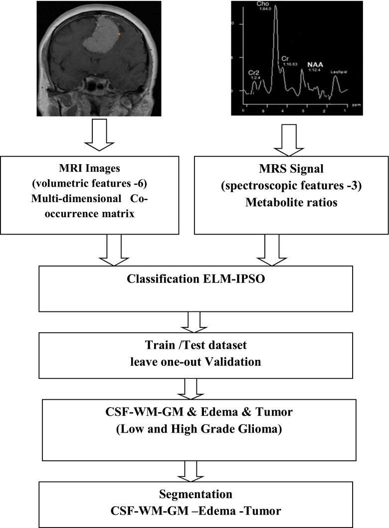
The key contribution of this approach constitutes the combination volumetric features extracted from the multidimensional co-occurrence matrices and spectroscopic features as modeled by the ratio between several metabolites. The volumetric and spectroscopic features are presented to the extreme learning machine-improved particle swarm optimization (ELM-IPSO) classifier [2] designed for head MRIs in the characterization of brain tissues along with significant amounts of pathological brain tissue as tumor. It also aids in the investigation on how the postcontrast magnetic resonance image and spectroscopic features might improve discrimination between high-grade and low-grade gliomas. The design model is shown in Fig. 1.

Fig. 1.

System design for both volumetric and spectroscopic features

Materials and Methods

MRI and MRS Clinical Specimens Acquisition

The clinical specimen utilized in the present study consisted of brain MR image series and MR spectra of 35 clinical routine cases with verified and untreated intracranial tumors; namely, 12 meningiomas and 23 gliomas. The MRI volumes acquired on a Siemens 1.5 T were available in two sequences: T1-weighted (T1) and T1 with gadolinium contrast agent (T1c). Each image sequence with a 3 mm brain slice-interval (i.e., the voxel size was 0.4492 mm × 0.4492 mm × 3 mm) in axial plane was measured. Regarding the acquisition of MR spectra, a single-volume spectroscopy of 1.5 T at short time echo (TE) (TE 10–25 ms/TR 500–1500 ms) proton MRS Imaging (1H-MRSI) sequence was used. To determine cerebral variation in MRS, area, amplitude, and ratios of major metabolites and spectral profiles are considered to detect differences in infiltration (N-acetyl-aspartate (NAA) — 2.02 ppm, NAA), proliferation (total creatine (tCr; 3.03 ppm))/choline-containing compounds ((tCho; 3.2 ppm)-Cho/Cr), necrosis (lipids), glycolytic metabolism (lactate), or energetic metabolism (glucose and glutamine) at different tumoral stages and after therapies. Spectroscopic VOIs were obtained from the T1-weighted postcontrast axial images, positioned entirely within the region of the tumor.

Volume of Interest Extraction and Feature Calculation

Second-order statistics tend to achieve higher discrimination indexes. Literature survey on texture analysis (TA) approach for MR images include gray-level co-occurrence matrix proposed by Haralick et al. [12] as most vastly used. Several promising studies have been analyzed with co-occurrence texture analysis in the classification of pathological tissues from normal tissues for example from the liver, breast, brain tumors with variable locations such as lymphomas, spine, and muscles with improvements [3]. Mahmoud et al. [22] have proposed a 3D approach using co-occurrence matrix analysis to increase the sensitivity and specificity of brain tumor characterization with promising results. Kovalev et al. [15–17] tested 3D co-occurrence matrices in analyzing cerebral tissue and glioma in T1-weighted MR images and analysis in age/gender related differences.

Failure of deformable models occurs due to presence of abnormal anatomical variability or even in the presence of normal but highly variable structures and accurate initialization [26]. Explicit anatomical templates have been successfully used through nonlinear registration, at high computational cost, and time complexity. Previous studies [2] indicate the use of subset feature selection methods to best describe the optimal features that result in high computational cost and limit in application to problems with high feature dimensionality. Hence, this work is proposed to develop a classification model with multidimensional co-occurrence matrix model that could aid in the automation of medical image analysis tasks by successfully segmenting both normal anatomy and tumor type pathology, with less computational time and complexity. To leverage the advantages and overcome the limitations of feature extraction and selection techniques, an integrated feature extraction and classification method for neuroimage classification is proposed. The model for 3D texture analysis is based on extended multidimensional co-occurrence matrices as in Kovalev et al. [15].

The 3D co-occurrence matrix describes image spatial structure based explicitly on the intensity information with no respect to other important features. Formulation of multidimensional co-occurrence matrix is a complex problem. The structure of M dimensional matrix is required to satisfy ‘the principle of orthogonal sets’ of elementary image features associated with different matrix axes. Research on texture dimensions [15] proved inclusion of properties like coarseness, contrast, periodicity, and anisotropy. Considering simultaneously all the features together with their variations in spatial domain, these image features could be accepted as an “orthogonal basis” for M dimensional co-occurrence matrix axes. The co-occurrence matrices are likely to be generalized to D dimensional Euclidean spaces and extract more characteristics from the matrix. Addressing different aspects of analyzing images into physiological and pathological interest requires classification using multiparameter values. Here, multiparameter features refer to the following three specific values for the edges (E), gray values (G), and local contrast (H) of the voxels [16]. The co-occurrence matrix describes local textural properties reasonably well, while the “global” image structure is almost ignored. These descriptors are insensitive to the global (low frequency) shape of a multidirectional 3D image pattern if the range of intervoxel distances is relatively small. Hence, the need for matrices to describe global structure with various other features and orientations is required. The inclusion of feature selection stage in the previous discussion forfeits faster recognition time. Hence, limited optimal feature selection is required for faster recognition rate. This section presents a feature extraction functioning based on multidimensional co-occurrence matrices. The effectiveness of the proposed approach is demonstrated through development of extreme learning machine-improved particle swarm optimization (ELM-IPSO) classifier for the same datasets.

Volumetric MR Imaging Features Using Multidimensional Co-occurrence Matrices

The enhancement of spatial dimensionality on the same set of discrete gray values modifies the relationships between the sets of possible dimensional images and their co-occurrence representations. The need to improve the sensitivity and specificity of co-occurrence features is essential to enable recognition and partition of numerous normal and pathological structures of textural differences in MR brain images. The spatial co-occurrence matrix dimensions (number of axes) in combination with basic image features (e.g., intensity, gradient magnitude, and orientation) result in improved multidimensionality matrix [15]. The image dimensionality corresponds to spatial dimensionality of input data, while the matrix dimensionality reflects the number of image characteristics and intervoxel relations under consideration [15]. The Laplace derivative and global neighborhood statistics add significance to the co-occurrence matrix.

Based on the previous works and literature studies [2] that have been carried out earlier, the feature space is modified as proposed in Kovalev et al.'s studies [15–17] that best describes the statistical behavior on the classification of brain tissue types. The attributes are:

• The magnitude of the local gradient magnitude (∇)

• The angle orientation (θ)

• The surface slope (Φ) (i.e., angle between reference and surface planes)

• The Laplace image derivative (L)

• The gray-level neighborhood intensity (NS)

• The Euclidean distance (D)

The co-occurrence matrix illustrates the MRI structure of 3D gray-scale segment. The detailed descriptors of spatial 3D image structure are a modification to the extended multisort co-occurrence matrices proposed by Kovalev et al. [15]. The value m of the matrix is the frequency of certain features of a given voxel pair. Consider a random voxel pair (i, j) defined on a discrete 3D voxel lattice i = (x_i,y_i,z_i) and j = (x_j,y_j,z_j) with Euclidean distance D (i, j). The Laplace image derivative on these voxels is represented as L(i, j), local gradient magnitudes by ∇(i, j), the angle between their 3D gradient vectors by θ(i, j), slope ɸ(i, j), and neighborhood statistics NS(i, j). Then, the general, six-dimensional co-occurrence matrix can be defined as:

1

Gradient magnitudes (i), δ(j), and angle between gradient vectors θ(i, j) are computed as:

2

where δ(i) × δ(j) is the dot vector product and δ(i) and δ(j) corresponds to the normalized gradient vectors. Gradient vector components ∇_x, ∇_y, and ∇_z can be calculated by any suitable 3D operator. In place of Zucker–Hummel filter in Kovalev et al.'s studies [15], a combination of (3 × 3 × 3 window) Sobel gradient and Laplace image derivative operator (first-order and second-order derivative) resulted in better performance. Neighborhood statistics, a simple geometric standard deviation of intensity around a voxel’s small neighborhood region, uses the logarithm of the intensity in contributing more informative space due to exponential distribution of image intensity. The gradient magnitude at the position of the Laplacian zero crossing combines information from multiple orthogonal operators in a vector space and then projects the results to the edge subspace. The co-occurrence matrix was normalized by the elements proportional to the brain region volume for each distance bin separately [15].

The structure of normalized multidimensional co-occurrence matrix dimensions includes intervoxel distance, intensity neighborhood, gradient magnitude, its relative gradient orientation (angle between gradient vectors), slope, and image derivative to form a set of fundamental image characteristics. The relativity of all features of the multidimensional matrix is invariant to translation, rotation, and reflection of image data. The local gradient magnitude appends information about the homogeneity of the local neighborhood, i.e., whether the region is rather uniform in intensity (e.g., in the white matter) or has high intensity slopes (e.g., at the gray/white matter border). The gradient angle θ(i, j) mostly captures gyral and sulcal shape variability. The image derivatives are converted to polar co-ordinates to retain the information. The texture analysis calculates gray-level co-occurrence matrix, which includes both global feature and local feature space. The gray-level co-occurrence matrix is computed at each phi, theta, and radius level. The six-dimensional co-occurrence matrices were computed for the anatomy structure, to recognize white matter, gray matter, cerebrospinal fluid, tumor, and edema with 45° spatial resolution of directions, i.e., x,y,z directions 3 × 3 × 3 − 1 = 27 − 1 neighbors in spatial directions. The co-occurrence matrices are respective of pairs and are irrespective of the actual directedness of the line between the elements of the pair. As a result, the half-size directional space is needed. The combinations of the spatial relationship or the displacement vector d are considered to set as four distances in 1, 2, 4, and 8 voxels and 13 directional spaces. The approach constructs features from the entire VOI. The proposed method results in a simple information fusion strategy which iterates between a 3D gradient feature with co-occurrence matrices, along with image derivatives and neighborhood statistics to identify brain tissues and classification step to identify the tumor pathology tissue.

Here, the following dimensions were binned as follows: four intensity bins (64 units each), six angle bins (45° each), and 20 distance bins (d = 20). Co-occurrence matrices are collected within a certain VOI and represented as a point in the six-dimensional feature space. The co-occurrence matrix is a combination of the occurrences of pairs of gray-scale values in the image, as a function of distance and direction. Usually the co-occurrence matrix of the image is tabulated with the number of times of specific voxel values that occur as neighbors in a specific direction. No repetition of voxel pairs is formed by every current image voxel and subsequent ones.

Spectroscopic Features

Magnetic resonance spectroscopy (MRS) measures the concentrations of different metabolite chemical components within tissues. From the spectroscopic data of each MRI, three metabolite markers of neuronal integrity were evaluated [choline (Cho), N-acetyl aspartate (NAA), and creatine (Cr)], and the following metabolite integral peak–height ratios were observed in the proposed pattern recognition system: Cho/NAA, Cho/Cr, and NAA/Cr [4, 11, 27]. These ratios are used in clinical practice for assessing various chemical properties of brain neoplasms, providing an added value in tumor identification [3, 4].

Model System Design and Evaluation

Classification was performed by starting with the more discriminative features and gradually adding less discriminative features along with spectroscopic features, until there is no significant improvement. For each dataset, the isolation in feature space (volumetric and spectroscopic) of the tumor classes, healthy brain tissue, and tumor brain tissue was evaluated. The extreme learning machine (ELM) algorithm proposed by Huang et al. [13] is determined. The input weights (v_i) and bias (b_i) are selected using improved PSO variant as in studies [2, 9] which adaptively adjust the corresponding network parameters. The output weights (β_i) are analytically determined based on the Moore–Penrose generalized inverse of the hidden-layer output matrix [2]. This modified ELM implemented the improved PSO and optimizes the input weights and hidden biases, according to both root mean squared error on validation set and the norm of the output weights [7]. The classification is performed for the selected feature sub-region as in Aruna Devi and Deepa’s study [2]. Pseudocode of the ELM-IPSO is given in Algorithm 1 [2, 9, 13].

Algorithm 1

Extreme learning machine-improved particle swarm optimization (ELM-IPSO)

• Step 1:

  Let the training set consist of N vectors, N = {(x_i,t_i)|x_i∈ Rⁿ_,t_i∈R^m, i = 1, 2,…N}.

• Step 2:

  Fix P hidden neurons with sigmoid function g(x) = 1/1 + exp[−(v × x + b)] for N different training samples.

• Step 3:

  Initialize population array of swarm particles with a set of input weights and hidden biases.

  P_i = [W₁₁, W₁₂,…, W_1n,…, W₂₁, W₂₂,…, W_2n,…, W_H1, W_H2,…, W_Hn, b₁, b₂,…, b_H] within range of [−1,1], modeling SLFN with output weights β as:

  3
• Step 4:
  Calculate hidden layer output matrix H using Eq. 4.

  4

  5
• Step 5:
  For each swarm particle, compute the fitness as the root mean squared error (RMSE) on the validation set only instead of the whole training set as used in Zhu et al.'s study [30] along with the norm of output weights.

  6

  7

  where fitness of best positions and their corresponding weights are considered. η > 0 is the tolerance rate.
• Step 6:
  The corresponding output weight matrix β is calculated with least-square Moore–Penrose generalized inverse of H (H†) using Eq. 8.

  8
• Step 7:
  The velocity updation is done as,

  9

  c₁ = c₂ = 2.05 [8], which scales cognitive and social components equally. Equation 10 represents β as the constriction coefficient.

  10

  where κ ε [0,1] and ψ = c₁ + c₂. κ is often set to 1 which is successful here.
• Step 8:
  The position of each particle is updated using Eq. 11, and a new population is generated.

  11
• Step 9:

  The algorithm is repeated until the criterion of hard threshold value is reached or maximum number of iterations is met.

  Once stopped, the algorithm reports values of g_best and f(g_best) as its solution. The best parameter values with γ_1,γ₂ = 0.5, N = 50, and maximum iterations of 200 are computed for selection of input weights and bias.

Statistical Experiments and Results

Due normalization was performed towards segmentation of VOI of the images. The multidimensional co-occurrence matrices represented the most discriminatory features for the segmentation of white matter, gray matter, CSF, and abnormal tissue separation. The MRS spectroscopic features provided additional information on the tumor grade present for the subject-specific abnormal tissue prior the MRSI data. All voxels under abnormal category were classified into the respective tumor grade that was represented in the training and test set for pattern recognition. The detection of white matter (WM), gray matter (GM), cerebrospinal fluid (CSF), tumor, and edema along with the spectroscopic profiles used for the classification of high-grade and low-grade gliomas was proved. Evaluation is done by leave-one-out validation analysis. A test set was used to calculate classification results for each dataset. In particular, the proposed ELM-IPSO classification system was designed and assessed by using solely (a) textural features or (b) spectroscopic features and (c) both textural and spectroscopic features [10]. Finally, mean classification accuracies and variances were evaluated at each number for all features.

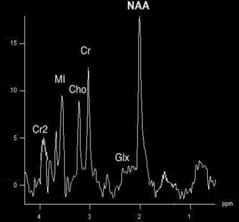
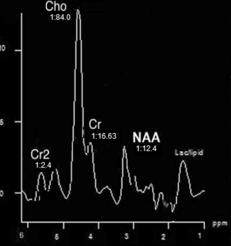
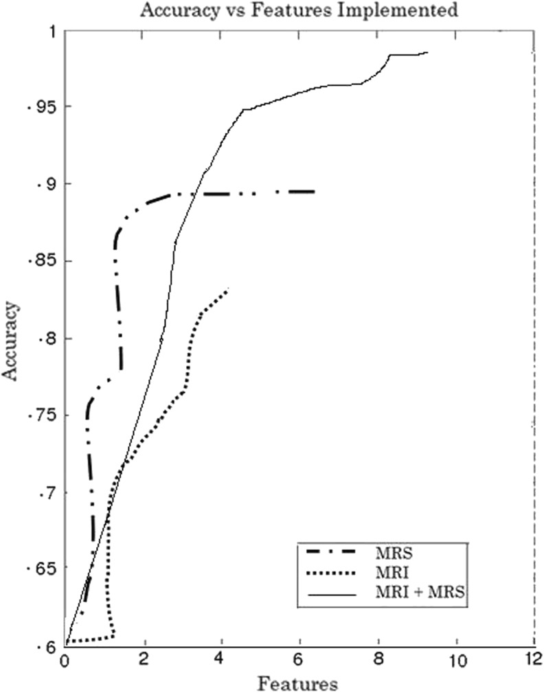
Table 1 shows the classification accuracy evaluation with various features implemented. To assess the precision of the proposed classification system, the co-occurrence matrices resulted in an overall discrimination accuracy of 86.5 %. Figures 2 and 3 depict MRS signal for normal brain and tumor brain. Together, both volumetric features and spectroscopic features proved the highest discrimination accuracy between low-grade and high-grade gliomas of 99.15 % as in Fig. 6.

Table 1.

Comparison of classification accuracy in the discrimination of low-grade and high-grade glioma

Features	Classification accuracy of low-grade glioma	Classification accuracy of high-grade glioma	Overall accuracy	Std Dev
MRI (textural)	88.45	84.20	86.50	6.8
MRS (spectroscopic)	92.65	89.35	90.5	7.2
MRI & MRS features	99.15	98.25	99.15	8.05
3D GLCM & RLM [2, 14]	93.05	95.65	94	7.4

Fig. 2.

MRS signal-normal brain

Fig. 3.

MRS signal-glioma

Fig. 6.

Accuracy vs number of features

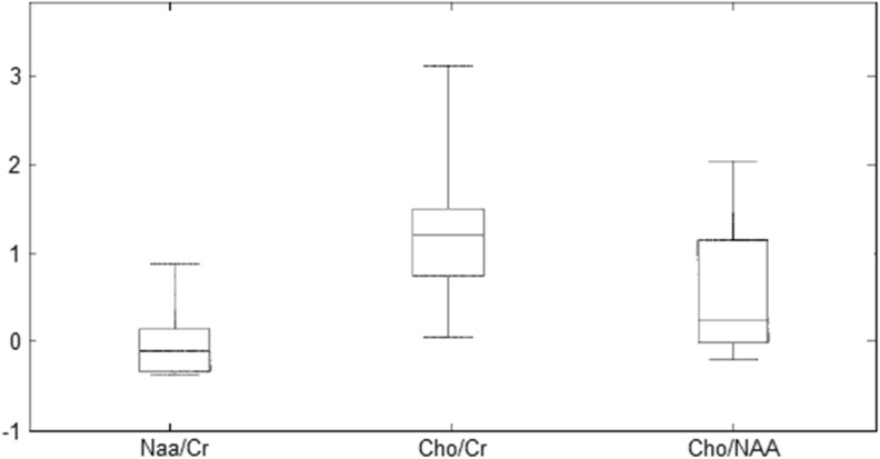
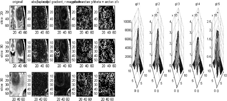
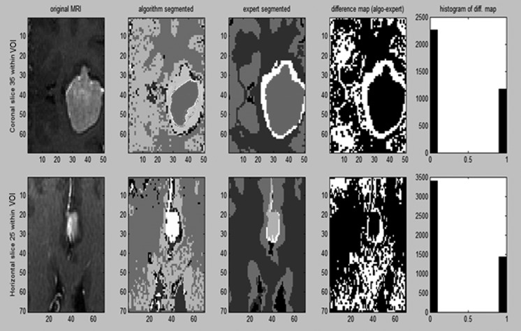
Figure 4 portrays the box-plots of resonance spectroscopic features resulted for glioma grade tumor. These multidimensional feature points are invariant to rotation, translation, scale, and viewpoint. The values of the vectors of co-occurrence matrices constructed for describing regional texture features, comprising intensities, their gradients, the angle between gradients, their gray-level neighborhood statistics, surface slope, distance, and Laplace derivative, are proposed. Here, the following dimensions were binned as follows: four intensity bins (64 units each), angle bins (45° each), and four distance bins (d = l–4″). Co-occurrence matrices were collected within a certain VOI and represented as a point in the six-dimensional feature space. The proposed method is compared with 3D GLCM–RLM features requiring additional features and, substantially, a feature selection stage [2, 11]. It has been noticed that the proposed system gives better sensitivity, specificity, and overall accuracy with 99.15 % as in Table 2 when compared with various neural classifiers. Figure 5 shows the volumetric features extracted on co-occurrence matrices. The spectral features enhanced the accuracy up to 90 %. Figure 6 illustrates the accuracy versus number of features. Figure 7 depicts segmented portion of tumor, edema, and brain tissues.

Fig. 4.

Box plots of spectral resonance features

Table 2.

Results on the proposed MRS and MRI COM model on various classifiers

Classifier	Sensitivity %	Specificity %	Overall accuracy %	ROC Az	MSE
BPN	89.58	68.17	82.85	0.81	0.21
SVM	91.84	76.19	87.14	0.90	0.10
ELM	93.33	86.533	93.5	0.94	0.09
IELM-PSO	98.01	95.0	99.15	0.97	0.015

Fig. 5.

Multidimensional co-occurrence matrix volumetric features

Fig. 7.

MRI segmentation: tumor, edema, CSF, WM, GM with expert validation

From the receiver operating characteristic (ROC), area under the curve (AUC) and related statistics are obtained and are tabulated as in Table 3. Apparently, the ELM has the highest AUC value, which indicates that it is the best classifier. The standard errors are reasonably small, resulting in relatively narrow confidence intervals. The lower limits of the confidence intervals of the AUC of the three classifiers exceed the 0.5 value (the AUC of a random classifier), and hence, the three classifiers perform much better than a random classifier. To compare the three classifiers, pairwise statistical t-test is applied based on the differences in the AUC of the three classifiers. The null hypothesis is that the difference in the AUC between two classifiers is equal to zero. The pairwise comparison in Table 3 between the ELM-IPSO versus SVM and IELM-PSO versus back propagation shows that their confidence intervals do not include the 0 value with p < 0.001, which means that in both cases the difference in AUC of the ROC is statistically significant. On the other hand, the pairwise comparison between the SVM versus the back propagation shows no significant difference between their AUC values since the confidence interval (CI) contains the 0 value with nonsignificant p value = 0.793. Thus, various statistical results significantly prove that the ELM-IPSO classifier has the higher classification accuracy.

Table 3.

Pairwise comparison between the AUC of the classifiers using Student’s t-test

	IELM-PSO vs SVM	IELM-PSO vs BPN	SVM vs BPN
MSE error	0.00954	0.0256	0.0102
95 % confidence interval (CI)	0.0854–0.134	0.0724–0.0154	−0.0179–0.032
Significance level	p < 0.05	p < 0.05	p = 0.793
Difference in AUC curve	0.08	0.03	0.02

Discussions and Conclusions

Choline found in cell walls increases as the cells replicate, evident in tumor case. Creatine, spectroscopic reference metabolite, tends to remain more or less constant throughout the normal state and most pathologic conditions. NAA, a neuronal health marker, tends to be lower in tumor case. Lipid and lactate locate on almost same spectrum signal and are markers of tissue necrosis. MRS is most useful in distinguishing tumor from other lesions that can look like a tumor on MRI. In all cases, the pathology from these locations demonstrated either the existence of tumor cells or their location in low-grade and high-grade gliomas. Hence, spectral pattern resembles patterns for grading in tumors. Further analysis of the misclassified cases showed that, in spite of validation, there were two glioblastomas where normal tissue contribution had overlapping of necrotic pattern with lipid signals at short TE. Hence, both long TE and short TE should be analyzed. Additional brain tumor patterns and grades can be analyzed using in-vivo and ex-vivo data.

Dissimilar types of tissue undergo intensity discrepancy of brain overlaps. This extends for any intensity-based discrete voxel labeling model. It reasons out due to the finite spatial distribution of the image acquisition: voxels at the boundary between tissue types have more than one tissue contributing to the measured signal (partial volume effect). The tumor edge voxels are situated in high-gradient regions of the MR image, which has been overcome by the proposed approach against [4]. The elimination of feature selection stage reduces the computational cost. The segmentation method using data fusion of MRI and MRS is only a simple information fusion strategy, but it is effective for tumor classification. Here, they act as image enhancement methods. MRS achieves a high degree of diagnostic specificity, since it is able to detect the biochemical changes that accompany specific diseases.

Comparing with the state-of-the-art techniques, Devos et al. [7] approach employed achieved 97 % discriminatory classification between metastatic and meningiomas using LS-SVM network. Luts [19] modeled LS-SVM classifier with 96 % accuracy towards grading of tumors. Similarly a recent model [11] attained 100 % accuracy with both textural and spectroscopic features using SVM in the discrimination of meningiomas and metastases. To overcome the limitations of the abovementioned 3D feature extraction and selection techniques (which involve more features) and previous findings [2], an integrated feature extraction and selection model for 3D texture analysis based on extended multidimensional co-occurrence matrices method for neuroimage classification is proposed in this paper. Hence, in comparison to the state-of-the-art models, studies using ELM-IPSO classifier have been experimented for its speed and simplicity [2], which produces the best generalization solution in real time domain application. Further computational time is reduced, due to elimination of feature selection stage, modeling a simple computationally efficient automated system design.

The current version of the proposed system could be extended for multifocal tumors. Further investigation on magnetic source imaging (MSI) with magneto encephalography (MEG) and brain mappings will assist in correlating intraoperative cortical simulation. Exploration towards brain mapping techniques will aid in neurooncology management featuring multi faceted purview. The thrust for studies towards stereotaxic space in MR images can be explored with new metabolite components [23].

References

- 1.Cancer Facts & Figures 2012. Atlanta: American Cancer Society; 2012. [Google Scholar]
- 2.Aruna Devi B, Deepa SN. Brain tumor tissue characterization in 3D magnetic resonance images using improved PSO for extreme learning machine. Progress in Electromagnetics Research B. 2013;49:31–54. doi: 10.2528/PIERB13010202. [DOI] [Google Scholar]
- 3.Alparone L, Argenti F, Benelli G. Fast calculation of co-occurrence matrix parameters for image segmentation. Electronics Letters. 1990;26(1):23–24. doi: 10.1049/el:19900015. [DOI] [Google Scholar]
- 4.Bendszus M, Warmuth-Metz M, Klein R. MR spectroscopy in gliomatosis cerebri. American Journal of Neuroradiology. 2000;21:375–380. [PMC free article] [PubMed] [Google Scholar]
- 5.Croteau D, Scarpace L, Hearshen D, Gutierrez J, Fisher JL, Rock JP, Mikkelsen T. Correlation between MRS imaging and image guided biopsies: semi quantitative and qualitative histopathological analyses of patients with untreated glioma. Neurosurgery. 2001;49:823–829. doi: 10.1097/00006123-200110000-00008. [DOI] [PubMed] [Google Scholar]
- 6.Chris C, Alex Zijdenbos P, Evans CA. A fully automatic and robust brain MRI tissue classification method. Medical Image Analysis. 2003;7:513–527. doi: 10.1016/S1361-8415(03)00037-9. [DOI] [PubMed] [Google Scholar]
- 7.Devos A, Simonetti AW, van der Graaf M, Lukas L, Suykens JA, Vanhamme L, Buydens LM, Heerschap A, Van Huffel S. The use of multivariate MR imaging intensities versus metabolic data from MR spectroscopic imaging for brain tumour classification. J Magn Reson. 2005;173:218–228. doi: 10.1016/j.jmr.2004.12.007. [DOI] [PubMed] [Google Scholar]
- 8.Fei H, Hai-Fen Y, Qing-Hua L: An improved Extreme learning machine based on particle swarm optimization. Proc. of Int. conf. on Intelligent Computing: 699–704, 2012.
- 9.Fuster Garcia E, Tortajada S, Vicente J, Robles M, García Gómez JM. Extracting MRS discriminant functional features of brain tumors. NMR Biomed. 2012 doi: 10.1002/nbm.2895. [DOI] [PubMed] [Google Scholar]
- 10.Garcia Gomez JM. Brain tumor classification using magnetic resonance spectroscopy. Tumors of the Central Nervous System. 2011;3:5–19. [Google Scholar]
- 11.Georgiadis P, Kostopoulos S, Cavouras D, Glotsos D, Kalatzis I, Sifaki K, Malamas M, Solomou E, Nikiforidis G. Quantitative combination of volumetric MR imaging and MR spectroscopy data for the discrimination of meningiomas from metastatic brain tumors by means pattern recognition. Magnetic Resonance Imaging. 2011;29:525–535. doi: 10.1016/j.mri.2010.11.006. [DOI] [PubMed] [Google Scholar]
- 12.Haralick RM, Shanmugam K, Dinstein I. Textural features for image classification. IEEE Trans. Syst. Man Cybern. 1973;3:610–621. doi: 10.1109/TSMC.1973.4309314. [DOI] [Google Scholar]
- 13.Huang GB, Zhu QY, Siew CK. Extreme learning machine: theory and applications. Neurocomputing. 2006;70(1):489–501. doi: 10.1016/j.neucom.2005.12.126. [DOI] [Google Scholar]
- 14.Howe FA. Opstad KS:1H MR spectroscopy of brain tumors and masses. NMR Biomed. 2003;16:123–131. doi: 10.1002/nbm.822. [DOI] [PubMed] [Google Scholar]
- 15.Kovalev VA, Kruggel F, Gertz HJ, von Cramon Y: Structural brain asymmetry as revealed by 3D texture analysis of anatomical MR images. Proc. of Int. Conf. on Pattern Recognition, Quebec: 808–811, 2002.
- 16.Kovalev VA, Petrou M, Suckling K. Detection of structural differences between the brains of schizophrenic patients and controls. Psy. Research: Neuro-imaging. 2003;124:177–189. doi: 10.1016/s0925-4927(03)00070-2. [DOI] [PubMed] [Google Scholar]
- 17.Kovalev VA, Kruggel F, von Cramon DY, Gertz HJ. Three-dimensional texture analysis of MRI brain datasets. IEEE Trans. on Medical Imaging. 2001;20(5):424–433. doi: 10.1109/42.925295. [DOI] [PubMed] [Google Scholar]
- 18.Luts J, Laudadio T, Idema AJ, Simonetti AW, Heerschap A, Vandermeulen D, Suykens JAK, Van Huffel S. Nosologic imaging of the brain: segmentation and classification using MRI and MRSI. NMR in Biomedicine. 2009a;22(4):374–390. doi: 10.1002/nbm.1347. [DOI] [PubMed] [Google Scholar]
- 19.Luts J, Heerschap A, Suykens JAK, Van Huffel S. A combined MRI and MRSI based multiclass system for brain tumour recognition using LS-SVMs with class probabilities and feature selection. Artificial Intelligence in Medicine. 2007;40(2):87–102. doi: 10.1016/j.artmed.2007.02.002. [DOI] [PubMed] [Google Scholar]
- 20.Luts J, Martinez-Bisbal MC, Van Cauter S. Molla, Piquer E, Suykens JA, Himmelreich K, Celda, UB, Van Huffel S: Differentiation between brain metastases and glioblastoma multiforme based on MRI, MRS and MRSI. Proc. of the IEEE International Symposium on Computer-Based Medical Systems (CBMS), New Mexico: 1–8, 2009b.
- 21.Majós C, Aguilera C, Cos M, Camins A, Candiota AP, Delgado-Goñi T, Samitier A, Castañer S, Sánchez JJ, Mato D, Acebes JJ, Arús C. In vivo proton magnetic resonance spectroscopy of intraventricular tumours of the brain. Eur Radiol. 2009;19(8):2049–2059. doi: 10.1007/s00330-009-1357-y. [DOI] [PubMed] [Google Scholar]
- 22.Mahmoud GD, Toussaint G, Constans JM, de Certaines JD. Three dimensional texture analysis in MRI: a preliminary evaluation in gliomas. Magn. Reson Imaging. 2003;21:983–987. doi: 10.1016/S0730-725X(03)00201-7. [DOI] [PubMed] [Google Scholar]
- 23.Nelson SJ. Analysis of volume MRI and MR spectroscopic imaging data for the evaluation of patients with brain tumors. Magnetic Resonance in Medicine. 2001;46:228–239. doi: 10.1002/mrm.1183. [DOI] [PubMed] [Google Scholar]
- 24.Simonetti AW, Melssen WJ, de Szabo Edelenyi F, van Asten JJ, Heerschap A, Buydens LM. Combination of feature-reduced MR spectroscopic and MR imaging data for improved brain tumor classification. NMR in biomedicine. 2005;18:34–43. doi: 10.1002/nbm.919. [DOI] [PubMed] [Google Scholar]
- 25.Soffietti R, Baumert BG, Bello L, von Deimling A, Duffau H, Fre’nay M, Grisold W, Grant R, Graus F, Hoang-Xuan K. Guidelines on management of low-grade gliomas: report of an EFNS–EANO* Task Force. European Journal of Neurology. 2010;17:1124–1133. doi: 10.1111/j.1468-1331.2010.03151.x. [DOI] [PubMed] [Google Scholar]
- 26.Simon KW, Kaus M, Jolesz FA, Kikinis R. Adaptive, template moderated, spatially varying statistical classification. Medical Image Analysis. 2000;4(1):43–55. doi: 10.1016/S1361-8415(00)00003-7. [DOI] [PubMed] [Google Scholar]
- 27.Weibei Dou, Aoyan Dong, Shaowu Li, Ping Chi, Jean-Marc Constans: Glioma Tissue Modelling by combing the information of MRI and in vivo Multivoxel MRS. Proceedings of Int. Conf. on Bioinformatics and, Biomedical Engineering (iCBBE2010), China:1–4, 2010.
- 28.Wang Q, Eirini Karamani L, Erickson M, Uday Kanamalla S, Vasileios M. Classification of brain tumors using MRI and MRS data. Proc. of SPIE. 2007;6514:65140S1–65140S8. doi: 10.1117/12.736969. [DOI] [Google Scholar]
- 29.Fan Y, Shen D. Integrated feature extraction and selection for neuroimage classification. Proceedings of SPIE. 2009;7259:72591U. doi: 10.1117/12.811781. [DOI] [Google Scholar]
- 30.Zhu QY, Qin AK, Suganthan PN, Huang GB. Evolutionary extreme learning machine. Pattern Recognition. 2005;38(10):1759–1763. doi: 10.1016/j.patcog.2005.03.028. [DOI] [Google Scholar]