Intracardiac Acoustic Radiation Force Impulse (ARFI) and Shear Wave Imaging in Pigs with Focal Infarctions

Abstract

Four pigs, three with focal infarctions in the apical intraventricular septum (IVS) and/or left ventricular free wall (LVFW), were imaged with an intracardiac echocardiography (ICE) transducer. Custom beam sequences were used to excite the myocardium with focused acoustic radiation force (ARF) impulses and image the subsequent tissue response. Tissue displacement in response to the ARF excitation was calculated with a phase-based estimator, and transverse wave magnitude and velocity were each estimated at every depth. The excitation sequence was repeated rapidly, either in the same location to generate 40 Hz M-Modes at a single steering angle, or with a modulated steering angle to synthesize 2-D displacement magnitude and shear wave velocity images at 17 points in the cardiac cycle. Both types of images were acquired from various views in the right and left ventricles, in and out of infarcted regions. In all animals, ARFI and SWEI estimates indicated diastolic relaxation and systolic contraction in non-infarcted tissues. The M-Mode sequences showed high beat-to-beat spatio-temporal repeatability of the measurements for each imaging plane. In views of noninfarcted tissue in the diseased animals, no significant elastic remodeling was indicated when compared to the control. Where available, views of infarcted tissue were compared to similar views from the control animal. In views of the LVFW, the infarcted tissue presented as stiff and non-contractile compared to the control. In a view of the IVS, no significant difference was seen between infarcted and healthy tissue, while in another view, a heterogeneous infarction was seen presenting itself as non-contractile in systole.

I. Introduction

A. Myocardial Infarction

Bogen et al. [1] notes that myocardial infarction is characterized by a localized increase in myocardial stiffness and decreased contractility that evolves over weeks after the infarction event. Increased wall stresses in the rest of the ventricle cause it to grow and thin, increasing dysfunction and the subsequent risk of heart failure. The infarcted tissue is replaced by collagen, forming a stiff, fibrous scar [2], [3]. Concurrent with scar formation, the ventricles may remodel to compensate for the thinned, scarred segments being unable to support wall stresses. Remodeling is a change in the size, shape, and function of the ventricle, and often a precursor to eventual heart failure.

Infarctions can be imaged with a number of modalities, including contrast-enhanced MRI [4]–[7], PET [8], computed tomography (CT) [9], and most commonly, echocardiography [10]–[12]. Echocardiography is used to diagnose wall motion abnormalities as an indicator for infarction, but does not distinguish dead myocardium from “stunned” [13]–[15] or otherwise dysfunctional myocardium. A means to distinguish necrotic, stunned, hibernating, edemic, and healthy regions of tissue in the emergency room could greatly improve diagnoses and management [16], [17].

B. Acoustic Radiation Force Impulse and Shear Wave Elasticity Imaging

The motional response of tissue to external forces can be used to infer information about the tissue’s mechanical or elastic properties. Acoustic Radiation Force Impulse (ARFI) imaging uses focused, 10–100 μs ultrasonic pulses to locally transfer momentum into the tissue via absorption. The tissue transiently displaces away from the transducer around the focus, and the relative magnitude of this induced displacement between different excitations can be imaged with high-frame rate ultrasound and used to make images of relative elasticity. Another way to characterize elasticity is to image at the propagation velocity of transverse (shear) waves through a medium. Under a linear, semi-infinite, purely-elastic assumption, the shear wave velocity is related to the shear modulus by $c_T=\sqrt{\mu /\rho }$, where c_T is the velocity in m/s, μ is the shear modulus in kPa, and rho is the density, in g/cm². This is known as Shear Wave Elasticity Imaging (SWEI), and acoustic radiation force (ARF) is a convenient way to generate shear waves within the ultrasonic field of view (FOV).

Cardiac elasticity imaging with these ultrasonic techniques and others has been an area of increasing interest for its potential in directly imaging the mechanical compliance of dysfunctional, infarcted or fibrotic regions of myocardial tissue [18]–[24]. These studies have all imaged a transient mechanical response with ultrasound to characterize myocardial stiffness. Kanai imaged the transient Lamb wave generated in the IVS in response to aortic valve closure, but the other work has required external excitation of the myocardium, either mechanically or with Acoustic Radiation Force (ARF). In order to generate a highly localized excitation, the animals’ chests were opened and the excitation transducer was coupled directly to the myocardium.

Intracardiac Echocardiography (ICE) holds promise for obtaining the proximity to the tissue needed to generate and track tissue response to ARF excitations. ICE is commonly used for function assessment and therapy guidance [25]–[29], and has already been shown to be feasible for cardiac ARFI imaging [30], [31]. Because the imaging transducer is located so close to the myocardium, less ultrasonic energy is needed to excite the tissue, and the response can be imaged without the clutter associated with imaging across the chest wall. This work uses an intracardiac implementation to explore the possibility of using Shear Wave Elasticity Imaging (SWEI) and Acoustic Radiation Force Impulse (ARFI) imaging to distinguish healthy myocardium from infarcted myocardium. While a transthoracic means to image cardiac elasticity with ultrasound would have the greatest clinical potential for diagnosing AMI, this implementation may benefit patients in procedures where ICE is already called for and the location of infarcted myocardium is of interest (transcatheter ablation or pacemaker lead placement, for example). Moreover, this work aims to explore the elastic appearance and behavior of infarctions in a closed-chest animal model.

II. Methods

A. Experimental Setup

All data presented were acquired with 10-French ICE catheters, either the Siemens Acuson AcuNav (Siemens Medical Systems, Mountain View, CA, USA) or the Biosense Webster SoundStar (Biosense Webster Inc, Diamond Bar, CA, USA), running on a Siemens S2000 scanner. Both transducers use the same 64-element, 7.25 MHz linear phased array, with a 7 mm aperture in azimuth, but the SoundStar has an additional magnetic positioning sensor in its tip. Demodulated in-phase and quadrature (IQ) ultrasound data from custom pulse sequences were recorded with matched ECG data from eight porcine subjects in compliance with protocols from Duke University’s Institutional Animal Care and Use Committee (IACUC). One of the pigs was used as a control, and the other seven were subjected to ischemia through a series of foam embolizations to the left anterior descending (LAD) coronary artery, designed to mimic chronic ischemia in the apical IVS and lead to heart failure, but which ultimately created a pathology more like acute myocardial infarction (AMI). Additionally, in all but one of the initial injections, foam was unexpectedly also delivered to the left circumflex (LCX) coronary, resulting in infarction of the LVFW as well. Unfortunately, four of the animals did not survive to the first follow-up study. The four remaining animals (three embolized and one control) comprise the cohort for the data presented here.

The ICE catheter was either fed through the right atrium into the right ventricle (RV), or inserted retrograde across the aortic valve into the left ventricle (LV). The animals were each imaged four times: once prior to the embolization, and three times following, over a time period of approximately 150 days. The first follow-up imaging session was at 40 ± 12 days after embolization, the second at 53 ± 11 days, and the final study at 130 ± 24 days. The catheter was placed in the LV only during the final imaging study for safety purposes, after which the animals were sacrificed and their hearts sent for contrast-enhanced MRI imaging and subsequent histology. Imaging planes were selected to view the ventricular free wall, either from the RV outflow tract or near the apex, as well as the IVS, under the condition that the tissue was at most 20 mm from the transducer face. In each view, up to three M-Mode and one 2-D datasets were collected. In each imaging session, at least one view of the IVS and one view of the RVFW were obtained. Where independent views of the IVS or RVFW could be obtained, additional views of the same wall were imaged, especially when the presence of infarction was suspected. A total of 196 datasets were collected across the 16 imaging sessions.

B. Custom Beam Sequences

The impulsive excitation was generated with a 6.15 MHz 400-cycle (65 μs) pulse, using a single focus selected to maximally intersect the myocardium throughout the cardiac cycle. Available foci were every 2.5 mm betwen 7.5 mm and 20 mm. Previous intensity measurements and thermal FEM modeling [32] (data not shown) indicated that for similar pulse sequences (15 mm focus and 6 MHz center frequency), the Mechanical Index (MI) is under 1.63, the I_SPPA was under 2000 W/cm² (derated at α=0.3), and tissue heating at the focus is low, 1.01°C over four seconds with 80 excitations per second. The I_SPTA will thus be as high as 10 W/cm² during transmission of ARF pulses at 80 times per second. The beams were repeated and steered in two different tracking schema, to make the two types of images. A summary of the parameters are found in Table I.

TABLE I.

Parameters for Imaging Sequences

Common Parameters
Center Frequency	6.15 MHz
PRF	9.12 kHz
Excitation Pulse Duration	64 μs
Excitation Focus Range	7.15 mm – 20 mm
Tracking Pulse Bandwidth	50 %
Tracking Transmit Focus	400 mm
Imaging Depth	40 mm
B-Mode Parameters
Field of View	90°
Beam Spacing	0.65°
M-Mode ARFI-SWEI Parameters
Excitation Steering Angle	0°
Tracking ROI	15° right of center
Tracking Lines	16
Tracking Duration	5 ms
Excitations per Ensemble	2
Ensemble PRF	40 Hz
Number of Ensembles	160
Synthesized 2D ARFI-SWEI Parameters
Excitation Steering Angles	−22.5° – +22.5°
Excitation Angular Spacing	2.7°
Tracking Duration 3 ms
Tracking ROI	16° right of each excitation
Tracking Lines per Excitation (ARFI)	1
Tracking Lines per Excitation (SWEI)	3
Number of Synthesized Images	17

1) M-Mode ARFI-SWEI Sequences

To generate high temporal sampling of the cardiac dynamics, the excitation beam was held in the same location and rapidly repeated to generate M-Modes of shear wave velocity and displacement magnitude. The tissue response was measured between 0° and 15° to the right of the center of the B-Mode field of view as the superposition of two identically-generated responses, each imaged at different lateral locations. A diagram of the tracking configuration is shown in figure 1(a). Four parallel tracking beams were simultaneously recorded at a maximum depth of 40 mm, repeated at 9.12 kHz for 5 ms following each excitation. The receive beams directions were rapidly modulated during tracking, such that each receive beam alternately sampled two locations at 4.56 kHz each, for a total of 8 tracked angles per excitation. The tracking locations were changed on the second excitation for a total of 16 tracking lines across the two excitations. The tracking transmit beams had a 6.15 MHz center frequency, and were focused at 400 mm to distribute transmit energy across the dynamic-receive-focused receive beam locations. The entire excitation-tracking ensemble was repeated 40 times per second for four seconds, with a 90° field-of-view B-Mode image acquired between each ensemble.

Fig. 1.

(a) Locations of the M-Mode ARFI-SWEI excitation and tracking regions. Four closely-spaced parallel tracking lines are rapidly steered between the two yellow tracking regions following the first excitation, and between the two blue tracking regions after the second excitation, for a total of 16 tracking lines. (b) Locations of the synthesized 2D ARFI-SWEI image sequence acquisition ROIs. Four parallel tracking lines cover 16 degrees to the right of each of the N excitation locations. In this work, N=17 and the excitations are spaced 2.66° apart.

2) Synthesized 2D ARFI-SWEI Sequences

An ECG-gated multi-beat synthesis method was used to generate sequences of 2D ARFI and SWEI images that image multiple locations throughout the cardiac cycle. Because the excitation-response ensemble takes at least 5 ms per line, each ARFI or SWEI image takes much longer to acquire than a B-Mode image; in moving or changing imaging targets, this introduces artifacts associated with the time delays between imaging each angle. To address this, custom sequences were written that change the order in which the angles are imaged on each successive beat. A diagram is shown in figure 2. Over a number of beats, each angle in the field of view gets imaged at each delay in the cardiac cycle. There are a number of ways to configure the modulation of angles and delays with ECG triggering, but we selected a method that uses 17 excitations per image, and synthesizes 17 images over a configurable time selected to cover approximately one beat to stay within the memory restrictions of our system. On the first beat, the excitation steering angle progressed from left to right in 2.66° increments at intervals of 1/17th of the R-R interval, starting on the first QRS complex at the leftmost beam (beam 1) and ending approximately on the following QRS complex with the rightmost beam (beam 17). B-Modes were acquired between each ensemble, and the delay between ensembles was set so that the last beam was acquired approximately a full beat after the first. On the second beat, the ensembles progressed from left to right again, but started at beam 2 on the QRS complex, and then acquire beams 3 through 17, followed finally by beam 1. The pattern continued as the third beat started with beam 3, the fourth with beam 4, and so on and so forth to the final acquisition, which excited first beam 17 on the QRS, followed by beams 1 through 16 over the final beat. The entire sequence actually took 34 heartbeats to acquire (rather than the minimum of 17), since the ECG trigger could not be configured to fire immediately following each set of 17 ensembles, requiring an extra beat between each acquisition set to reset. To track the on-axis (ARFI) and off-axis propagation (SWEI) from each excitation, four receive beams were used, one aligned with the excitation, and the other three spanning 16 degrees to the right of the acquisition, as shown in figure 1(b). To reduce respiration motion artifact in the synthesized image sequences, respiration was temporarily held during acquisition. More lateral locations or time steps could not be synthesized with this setup, since our 17-time, 17-push-location image sequences generated the largest files that could be saved by our scanner (200 MB).

Fig. 2.

The ECG-triggered acquisition scheme used to synthesize 2D ARFI and SWEI image sequences. Each box represents an acquisition, indicating the order in which the scan lines are excited and tracked. The width of each box is the total time to acquire all N scan lines in each acquisition. T is the RR-Interval, and the vertical black lines represent ECG trigger signals. The work in this paper uses N=17.

C. Shear Wave Speed Estimation

A phase-shift based displacement estimator [33] was used to calculate the ARF-induced axial displacements, using a 1.5-λ kernel, progressively calculating the displacements between each successive pair of frames in the ensemble. To calculate the total displacement from the pairwise estimates, the stepwise displacement estimates were integrated. Once the displacements had been calculated, a third-order polynomial motion filter was used to remove the bulk axial motion of the tissue from the ARF-induced displacements [34]. For each ensemble in the M-Mode data, the temporal displacement estimate profiles were linearly interpolated up to 9.12 kHz to fill in the missing time steps due to the steering angle modulation. These displacement data, when tracked at the same steering angle as the excitation, are referred to as Acoustic Radiation Force Impulse (ARFI) displacements, while the rest of the data are used for velocity estimation.

At each depth and steering angle, the time to peak slope, or arrival time, was estimated using a sub-sample peak estimator that fit a quadratic polynomial to the peak rise in displacement and its temporally-adjacent estimates. Spatio-temporal samples corresponding to shear wave speeds less than 0.5 m/s or greater than 8 m/s were not considered when selecting the peak value. Simple linear regression was performed on all of the arrival times at each depth to obtain an estimate of the transverse wave velocity [35]. These velocity estimates are also referred to as Shear Wave Elasticity Imaging (SWEI) [36] and shear wave speed estimates. The estimation process was repeated independently for each repeated excitation ensemble. The M-Mode sequences formed 470 × 160 pixel M-Mode images through depth and across multiple heartbeats, to which a 5 × 3 pixel median filter was applied to remove outliers. For the synthesized 2-D images, the ARFI and SWEI estimates from each response were sorted to form sets of data, where each set contained all of the responses for a given ECG trigger delay, one at each lateral steering angle. For all of the ensembles acquired with the same delay, each shear wave speed estimate was assigned to the 15° ROI from which it was calculated and overlapping estimates for each lateral line were averaged together, weighted by the magnitude of their complex cross-correlation coefficients. The ARFI data did not overlap, so were assigned directly to their lateral location.

D. Multi-beat Synthesis

To compile the data acquired across multiple heartbeats, a technique called multi-beat synthesis [37] was used to register estimates from many frames onto a single heartbeat. Using matched ECG data, each displacement and velocity estimate was registered to the preceding QRS complex, placing all estimates on a single beat. For the 2-D image sequences, this resulted in a single estimate at each combination of steering angle and cardiac phase, making a series of seventeen, 470 × 17 pixel (pre-scan-conversion) ARFI images. SWEI images were similarly formed, but had an additional 16° in their field of view due to the extent of the rightmost tracking kernel (figure 1(b)), which resulted in 470 × 23 pixel images. For the M-Mode sequences, the 160 temporal samples cover the all phases of the cardiac cycle for the center steering angle. Forty evenly spaced time bins were used to subdivide one heart cycle, with each of the 160 estimates placed into the nearest bin. The estimates within each bin were then averaged together, weighted by their correlation coefficients, to form two 470 × 40 pixel M-Modes, one for ARFI displacement and one for shear wave speed.

E. Model Fitting

To form a more quantitative comparison among M-Mode images, 10 averaged profiles of displacement and velocity were computed from each synthesized M-Mode. The borders of the tissue were drawn by hand using the center line of the B-Modes for guidance, and the profiles averaged between deciles spaced between the axial boundaries so that each profile followed the same piece of axially-moving myocardium. Each of the 10 ARFI or SWEI profiles was then fit to a simple, six-parameter piecewise-linear model. The parameters were diastolic value, systolic value, end-diastole time, diastolic-systolic transition time, systolic duration, and systolic-diastolic transition time. A shear wave speed temporal profile for a single location and its corresponding model are shown in Figure 3. During diastole and systole, the model is constant, and during the transition times, the model is linear. MATLAB’s fit function was used, implementing a constrained, robust, nonlinear least squares Levenberg-Marquardt algorithm to do the fitting. The model is simple, but allows a numeric comparison between large amounts of data contained in each M-Mode. The parameters of interest reported in this work are the diastolic and systolic values.

Fig. 3.

Single-depth shear wave speed temporal profile with the simple model overlaid. The model parameters are fit to the means at each time step.

III. Results

Over all animals and all imaging sessions, 154 M-Mode images and 42 2-D image sequences were acquired in various views of the left and right ventricle. The results presented here are a subset of the views for which lateral tissue motion and the imaging angle were comparable.

A. Left Ventricular Free Wall Infarction

Figure 4 shows a single frame of the B-Mode clips acquired in the LVFW of one of the infarcted pigs on the left and the control pig on the right. The left image shows a large focal infarct in the LVFW, while the right image is nearly the same view, but shows no signs of damage. ARFI and SWEI estimates will be compared in the data acquired from these views.

Fig. 4.

B-Mode frames of the LVFW. The left image is taken from one of the infarcted pigs 126 days after infarction, and shows a large focal infarct in the frame. The right image, from the control (146 days after its sham procedure), shows the same view, but without any infarction. The yellow line indicates the steering angle of the ARF excitation for the M-Mode sequences.

Figure 5 shows the M-Modes of displacement magnitude and shear wave speed for the control pig’s LVFW over six beats. The axial and temporal trends in shear wave speed and velocity are highly repeatable from beat to beat and correspond with the associated ECG. It is also of note that depth variation is seen in the SWEI image but not in the ARFI image.

Fig. 5.

SWEI (top row) and ARFI (middle row) M-Modes of the LVFW from the control animal, with the corresponding ECG (bottom row). Data were taken 146 days after the first imaging date. High shear wave speeds and low displacements (yellow and cyan, respectively) correspond to stiff myocardium in systole, and slow speeds and high displacements (magenta) correspond to compliant myocardium. Desaturated pixels correspond to points outside of the depth of field and those with low complex cross correlation coefficients. In each of the six beats, the axial and temporal trends in both ARFI and SWEI measurements are highly repeatable.

Figure 6 shows six frames from the multi-beat synthesis 2-D SWEI and ARFI image sequence for the same view shown in Figure 5. A similar trend of elevated shear velocities and suppressed displacements are seen during systole, compared to diastole. Dimmed pixels, which show the underlying B-mode, correspond to low cross correlation coefficients or regions outside of the myocardium.

Fig. 6.

SWEI (top row) and ARFI (middle row) images of the LVFW from the control animal at various points in the cardiac cycle, displayed over the corresponding B-mode images, with the associated ECG trace (bottom row). Similar speeds and displacement trends are seen as in Figure 5, with general spatial uniformity and temporal contraction. Transparent colored pixels correspond to low cross correlation coefficients.

Figure 7 shows the SWEI and ARFI M-Modes for the two views in Figure 4 after multibeat synthesis, along with the associated ECG and (uncalibrated) LV pressure curve. The diastolic speeds appear elevated in the infarction compared to the control, and the displacements are correspondingly lower in the infarction. A small amount of relaxation is seen in the infarction from 350–500 ms.

Fig. 7.

Multibeat-synthesized SWEI (top row) and ARFI (middle row) M-Modes of the LVFW. The left images are taken from an infarcted region of Pig #2 126 days after infarction, and the right are taken from the control animal at 146 days after a sham procedure. The bottom row shows the associated ECG and pressure traces. Elevated diastolic shear wave speeds and corresponding lower ARFI displacements are seen in the infarction. Thin, dotted white lines delineate the axial tissue boundaries from all contributing beats, such that overlapping lines indicate repeatability of the axial tissue motion between beats.

Box plots are shown in Figure 8 for the model parameters fit to the data in figures 7 and the rest of the datasets from those views. Statistically significant difference in the means at the 5% level is indicated by the shear wave speeds for all Infarct-Healthy pairs except “Infarct 2” and “Healthy 3”. In the ARFI displacement data, statistical significance is only indicated between “Infarct 2” and “Healthy 1” and “Infarct 2” and “Healthy 2”.

Fig. 8.

Model parameters fit to each of the datasets acquired of the LVFW view during the final imaging study. Error bars indicate the standard deviation across the LVFW for 10 independent model fits. Data from the control pig, labeled “Healthy”, show higher contractility than those from the infarcted pig in both ARFI and SWEI.

Figure 9 shows the same frames from the 2D sequence as Figure 6, but for Pig #2 with the infarcted portion of the free wall shown in Figure 7. Images were taken 126 days after infarction. The displacements and velocities remain low and high, respectively, throughout the cardiac cycle. During mid diastole, a small region of elevated displacements is seen in the infarct, shown by the magenta region in the upper right portion of the images at 412 ms.

Fig. 9.

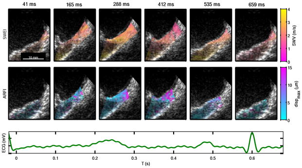
SWEI (top row) and ARFI (middle row) frames from the synthesized 2-D image sequence of a region of infarcted LVFW, and the corresponding ECG (bottom row). The infarcted tissue maintains low displacements and high velocities throughout the cardiac cycle, indicating that it is stiff and non-contractile. During mid-diastole (412 ms), a small region of higher displacements and lower velocities seen in the upper right part of the image

B. Intraventricular Septum Infarction

A comparison of ARFI and SWEI data imaging healthy and infarcted myocardium within the same animal is shown in Figure 10. The tissue in the infarcted region was thinned, and presented a conduction delay in the B-Mode. The ARFI and SWEI M-Modes, however, show no apparent change along the lines measured. The healthy tissue shows strong shear wave speed variation transmurally through the septum.

Fig. 10.

Multibeat-synthesized M-Mode SWEI (top row) and ARFI (middle row) of the IVS for an infarcted region (left) and spared region (right) of the same animal 140 days after infarction, with traces of ECG and relative pressure (bottom row). The spared region indicates potential transmural anisotropy, while the infarcted region does not. Though thinned in the infarct, peak contractility appears similar in both tissue samples, and both regions show diastolic compliance.

Figure 11 shows the box plots for the views of the IVS shown in Figure 10, along with the other two repeated acquisitions at each view. No statistically significant differences are seen, although the shear wave speed ratios seem to have lower bounds in the spared tissue, and the ARFI ratios seems to be somewhat higher in the spared tissue.

Fig. 11.

Model parameters fit to each of the datasets acquired for the IVS views shown in Figure 10. Error bars indicate the standard deviation spatially across the septum for 10 independent model fits. SWEI data indicate higher variation in the larger, spared region, but higher ratios in the thinned region, while ARFI data indicate higher, though not significantly so, ratios in the spared region.

C. Remodeling

The ejection fractions for the pigs, from three views, are presented in table II. All of the animals, including the control, had a moderately decreased ejection fraction 9–10 days after the embolization. Data from the later studies are not available.

TABLE II.

Ejection Fraction Measurements

Ejection Fraction (%)	Pre-embolization	9–10 Days Post-embolization
Pig 1	58.3 ± 8.1	54.7 ± 5.9
Pig 2	52.5 ± 7.6	51.0 ± 2.6
Pig 3	51.0 ± 8.5	40.7 ± 6.7
Pig 4 (Control)	54.3 ± 3.2	46.0 ± 3.0

The diastolic shear wave speeds, taken from the model fits to all datasets in both the RVFW and the IVS, are shown in figure 13. In all but Pig #1, the diastolic shear wave speed increased with significance p<0.05 by the final imaging study, including the control animal. In the RVFW, none of the diastolic shear wave velocities were increased at the final imaging study.

Fig. 13.

Diastolic shear wave speeds in the IVS (a) and RVFW (b) for the four animals over 150 days. Stastical significance in a Student’s two-tailed T-Test is shown relative to the first imaging session for each animal, and demarcated with an asterix.

Cross-sectionally, comparing all of the views of the IVS from the final imaging study between all of the animals, no difference were seen in diastolic shear wave speeds between pigs. The animals with infarcts had diastolic speeds of 1.289 ± 0.033, 1.354 ± 0.029, and 1.366 ± 0.059 m/s, respectively, while the control animal had diastolic speeds of 1.420 ± 0.042 m/s. If anything, the average diastolic velocities for the control are a bit higher that the infarcted estimates, but grouping the infarcted animal estimates together, and performing a one-way ANOVA against the control, the means are not significantly different (p = 0.058).

Individual views of non-infarcted septum were also compared across the four pigs. The most common view was of the IVS, and multibeat-synthesized M-Modes of the IVS are shown for the four pigs in Figure 14. Substantial remodeling is not apparent in the ARFI or SWEI data, as clean contractility with similar shear wave speeds is observed. A statistical analysis by one-way ANOVA indicates no difference in the diastolic means between the infarcted animals and the healthy (all infarcted c_dias = 1.444 ± 0.059 m/s, control c_dias = 1.414 ± 0.102, p = 0.801).

Fig. 14.

Multibeat-synthesized M-Mode SWEI (top row) and ARFI (middle row) of the IVS for the four pigs, with associated ECG and pressure traces (bottom row). Images were acquired at the final imaging session for each animal (140, 126, and 105 days after infarction, respectively, for Pigs #1–3, and 146 days after the sham procedure for the control). No global remodeling is indicated between the spared regions of the IVS in the infarct animals (left three columns) and the healthy tissue of the control (rightmost column).

Figure 15 shows the box plots for the model parameters fit to the data in Figure 14. Pig “infarct 3” has higher contractility than the control in the ARFI ratio, but not the SWEI ratio, and none of the other diseased pigs showed significant differences in either measurement.

Fig. 15.

Model parameters fit to the datasets acquired from spared septum in the four animals during the final imaging studies. Data from the diseased pigs, labeled “Infarct”, show no significant signs of remodeling, compared to the control. The ARFI data show Pig #3 to have significantly higher ARFI ratios than the control. Error bars indicate standard deviation across the septum among 10 independent model fits.

D. Heterogeneous Infarction

In one of the animals, views were obtained of a thinned region of apical septum from the LV. The catheter was able to be drawn back, moving the field of view to more basal, spared septum. At approximately 5 mm intervals, images were taken. A diagram of the approximate imaging locations is shown in Figure 16. The B-Mode shown is from the center of the three locations.

Fig. 16.

B-Mode image of the IVS, with spared septum on the left (basal), and infarcted septum on the right (apical), taken 126 days after infarction in Pig #2. The three lines indicate the imaging locations for the M-Modes.

Figure 17 shows the SWEI and ARFI M-Modes recorded for the rightmost line in Figure 16. Transmural variation of ARFI and SWEI is seen during systole in each beat, with more spatially-uniform values in diastole. These features are present in each beat of the M-Mode. Figure 18 shows the multibeat-synthesized SWEI and ARFI M-Modes for the three locations indicated in Figure 16. The most basal (spared) image is on the left, and the most apical (infarcted) is on the right (the synthesis of Figure 17. The spared septum shows uniform contraction transmurally, while the infarcted septum is thinned and shows transmural variation in the stiffness and contractility properties. The RV side of the IVS in the right image maintains high displacements and low shear velocities throughout the cardiac cycle.

Fig. 17.

SWEI (top row) and ARFI (middle row) M-Modes of the septum and the corresponding ECG trace (bottom row), recorded at the rightmost (cyan) line indicated in Figure 16. Both ARFI and SWEI measurements indicate transmural heterogeneity during systole and axially uniform estimates in diastole, 126 days after infarction. These spatio-temporal trends are visible in each beat.

Fig. 18.

Multibeat-synthesized SWEI (top row) and ARFI (middle row) M-Modes of the septum, at the locations indicated in Figure 16, with corresponding ECG and pressure traces (bottom row). The apical septum is thinned and shows transmural variation in systolic stiffness in both ARFI and SWEI measurements for the center and apical views (middle and right columns) 126 days after infarction.

Figure 19 shows images from the 2D synthesized sequence for the view from Figure 16. The spatio-temporal nonuniformity is highlighted in this view, as the LV and basal regions of the image contract in systole, while the apical RV side remains compliant. Visual registration of laterally moving tissue is readily possible with the 2D field of view.

Fig. 19.

SWEI (top row) and ARFI (middle row) frames from the 2-D image sequence of a heterogeneously-infarcted region (Figure 16), and the corresponding ECG trace (bottom row). In the ARFI images, the RV side of the IVS near the apex does not contract during systole, showing elevated displacements, while the LV side of the IVS contracts and relaxes normally

IV. Discussion

We were able to use ARF delivered by an ICE transducer to generate and track transient displacements and resultant shear waves through systole and diastole in an animal model. In 122 of the 154 M-Mode images, clear trends of higher displacements (increased compliance) during diastole and lower displacements (increased stiffness) during systole were observed. In the remaining 32 images, no cyclic variation was seen- the images had either low displacements within the myocardium through the entire cardiac cycle, or low cross-correlation coefficients indicating motion. In 104 of the 122 M-Modes with cyclic ARFI displacements, the matching SWEI images showed clear trends of increased shear wave speeds in systole and decreased speeds in diastole. The high beat-to-beat repeatability facilitated multi-beat synthesis, and the results allowed us to observe interesting spatio-temporal abnormalities in the infarcted myocardium. The ARFI data showed a clean signal indicating at least some systolic contraction in a higher number of M-Mode images than the matched SWEI images (79% vs 68%), due to the additional step of estimating the transverse wave velocity. ARFI images showed less sensitivity to myocardial fiber orientation than SWEI images, since we were only able to measure the shear wave propagation in a single direction. The combination of both ARFI and SWEI allowed us to separate changes in substrate stiffness from variations in relative fiber orientation, which, without three dimensional tracking of wave propagation, is not possible with shear wave imaging alone.

A. Left Ventricular Free Wall Infarction

In the two views of the LVFW, high shear wave speeds and little contraction were seen in the infarcted region compared to the healthy tissue. The relatively higher variance of the ARFI estimates for the healthy tissue (Figure 8) is due to depth of field and attenuation effects over the much larger axial thickness of the free wall, which extends beyond 20 mm. Figure 5 shows that the axial and temporal trends through the LVFW and across the heart cycle are shown with high beat-to-beat repeatability. Looking at the upper end of each box for ARFI or SWEI in Figure 8 indicates large differences between the infarcted and control tissues in terms of the spatial peak contractility. The 2-D image sequences (Figures 6 and 9) show the relative spatial homogeneity of each of the tissue regions. The 2-D SWEI images have low resolution due to the averaging of overlapping 16° ROIs, but with the higher-resolution ARFI images do provide insight into the azimuthal distribution of stiffness. Interestingly, in the healthy tissue, a gradient is visible with depth during diastole, potentially indicating somewhat increased stiffness towards the epicardium. These low displacements and elevated velocities at depth during diastole are seen in the deep parts of Figure 7 as well. This may indicate that the epicardial part of the myocardium is more rigid than the endocardium, but effects of boundary conditions and ARF penetration depth obfuscate a stronger conclusion.

B. Intraventricular Septum Infarction

The views of the IVS (Figure 10) show a primarily negative result for distinguishing what appeared to be infarcted tissue from normal tissue within the same heart by ARFI and SWEI. The shear wave speeds and ARFI displacements in the thinned myocardium seem to follow the same contraction and relaxation of the spared region. A number of factors complicate this conclusion, however. First, the IVS displays transmural anisotropy in the shear wave speed images of the spared region, but not in the infarcted region. The band in the middle of the spared septum shows low shear wave speeds and low displacements during systole, while no such region exists in the presumed infarct. This causes the average systolic shear wave speed to be lower, and the standard deviation to be higher, in the spared region, which are both seen in figure 11(a). The ARFI ratios, on the other hand, appear somewhat higher in the spared septum, though statistical significance is not acheived. Neither of these change the fact, however, that the thinned region region of myocardium is compliant during diastole with shear wave speed near 1 m/s. We hypothesized that this could be stunned or hibernating myocardium, which would be dysfunctional without being fibrotic. Although the tissue may not actively contract itself, the contraction of adjacent, healthy tissue may stretch this tissue, creating the systolic stiffness. However, neither the ex vivo MRI (figure 12), nor the histological staining (not shown) indicated that Pig #1 had a thinned region of its septum that was not infarcted. The existence of this apparent “soft infarction” warrants further study to determine whether it is the result of an imaging artifact or a real pathology.

Fig. 12.

Slices of the ex vivo contrast-enhanced MRI volumes. The right ventricles were distended in the fixation process, but infarcts are clearly visible in the IVS of Pigs 1–3, as well as the LVFW of pigs 2 and 3.

C. Remodeling

Over the course of the study, we observed a small stiffening of the IVS during diastole in two of the three infarcted pigs as well as the control, and no significant change in RVFW diastolic stiffness, leading us to believe that we either did not acheive, or were not able to detect diastolic heart failure in these animals. The ejection fractions (Table II) did not differentiate the infarcted animals from the control at 9–10 days post-embolization, although in the later studies regional akinesis of the infarct areas was observed, and expected to have decreased the EFs below normal, though those data are unavailable. Additionally, cross-sectionally comparing all of the diastolic shear wave speeds in regions of spared IVS during the final imaging session, no signs of elevated diastolic stiffness were present in the SWEI data for the infarcted animals. Comparing similar views of the septum (Figure 14), we see variation, but no significant differences between the spared regions of the infarcted pigs and those of the control. The average diastolic velocities were nearly identical (1.414 m/s in the control, 1.444 m/s in the infarcted animals, p = 0.801). Figure 14 shows the M-Modes taken of the IVS, and we can see that the exact imaging plane varies between the views. The variation introduced by different imaging angles and targets indicates the importance of obtaining measurements of the same part of the tissue, at the same angle, for performing matched comparisons. Perhaps the strongest conclusion to be made from these data is that the heart is not mechanically homogeneous and that substantial regional variation exists even in healthy hearts. To make the truest comparison between diseased tissue and healthy, either the imaging planes need to be closely matched, or a map of regional properties needs to be created that can be aligned and registered between subjects.

D. Heterogeneous Infarction

In Figures 18 and 19, ARFI and SWEI agree on the decreased systolic stiffness of the RV side of the IVS near the apex, so the variation cannot be attributed simply to anisotropy. This result, like the other IVS result, was surprising, as it was expected that the thinned myocardium would be stiff and non-compliant throughout the cardiac cycle. Ex vivo contrast-enhanced MRI indicated the apical septum to be infarcted, but aligning the specific ultrasound viewing angles to the MRI data was not possible due to deformations introduced in fixing the heart for scanning. It is possible that the ultrasound imaging plane intersected infarcted, viable, or a mix of both types of tissue at different stages of the cardiac cycle. This infarcted region of the IVS may have been subjected to passive tension as the surrounding tissue contracted, such that the increase in stiffness on the LV side during systole was due to stretching rather than muscular contraction. Another confounding factor was substantial lateral motion of the septum in these images. The tissue moved back and forth underneath the ROI, and in the apical image, the ROI approached the apex itself at the peak lateral motion. Looking at the 2-D images, however (Figure 19), clear elastic distinction between the RV and LV sides of the septum was observed during systole in the ARFI images, and the moving septum is readily followed through the frames.

E. Limitations

To limit the anesthesia time of the animals, the data acquired were processed offline after each experiment. Single 2-D diastolic ARFI-only images were typically acquired before each set of M-Mode and 2-D ARFI and SWEI images to determine the appropriate focal configuration to use, but feedback on the quality of the acquired data was limited during the experiments. Images were typically acquired in whatever views situated the tissue within 2 cm of the transducer face with limited perceived motion, but the porcine cardiac anatomy created challenges in catheter positioning, and in some cases, the only available views of the septum or free wall had a large amount of motion.

Lateral and elevational wall motion, particularly during contraction and active relaxation, created decorrelation in the tracking data, which reduced the confidence of the displacement estimates and subsequently-calculated velocities. In the images shown, the saturation of each pixel is tied to the cross correlation coefficients of the contributing excitation-tracking ensemble, and low cross correlation coefficients exponentially de-weight the saturation, showing more of the underlying B-Mode, such as in Figure 17. This occurs in blood and in regions of high motion. The tissue is outlined with small dotted white lines in the M-Modes to show the tissue boundaries, but in the 2-D images, the blood signal was manually masked out, rather than just using the correlation coefficients. When making multi-beat synthesized M-Modes, the multi-beat averaging was weighted by the correlation coefficients to reduce the effect of outliers, but the motion from beat to beat is so repeatable that decorrelated pixels were often averaged with the also-decorrelated pixels from the following beats, as in Figure 18. Real-time guidance of ARFI and SWEI will aid future studies in imaging plane alignment, particularly with respect to fiber orientation. Additionally, as the heart beats, the angle between the ARF excitation and the tissue may change with cardiac motion. In the M-Mode images, this may mean that a different part of the tissue is imaged in systole than in diastole. While the multibeat-synthesis 2D image sequences address this, some M-Mode results could be subject to potential artifacts caused by the lateral and elevational heterogeneity of the tissue around the focus.

The effect of fiber orientation, was more of a confounding factor on the shear wave speed data than was initially expected. While ARF excitations occur mostly perpendicular to fibers, shear wave propagation is tracked by a linear phased array in a specific dimension, which can be parallel or perpendicular to the fiber orientation. ARFI was therefore less affected than SWEI, and in cases where the shear wave speeds varied without a corresponding change in the ARFI, we expect to be imaging fiber orientation variation rather than substrate stiffness changes. Future studies of shear wave speeds and myocardium will have to control for relative fiber angle closely, or else move towards tracking the wave propagation in 3-D, which would allow the anisotropic shear wave propagation to be imaged in all directions.

Beyond anisotropy, frequency dispersion affects the generalization of the shear wave speed estimates. In some views, the myocardium is less than 5 mm thick, whereby a shear wave model may not be appropriate, as the tissue may be excited in an antisymmetric Lamb wave mode. Nenadic et al [38] describe an approach for modeling such dispersion. In addition to boundary condition-induced dispersion, myocardium is expected to exhibit a degree of dispersion associated with its viscoelastic properties as well. How these properties provide different information than the basic group velocity approach used here will also need to be explored in future work.

Perhaps the greatest limiting factor, however, is the limited range of imaging. Because the AcuNav is such a small probe, it was difficult to generate and track shear waves at depth. Whereas images were acquired with up to a 45° field of view down to 4 cm, images with excitation foci beyond 15 mm were less successful at generated distinct shear waves than those which used transmit F-numbers less than 2. This limited the usable field of view to a small region, which in turn limited the amount of the heart that could be characterized in any single image. Some views did show spatial variation within the small window (Figure 19, for example), but we predict that the capabilities of the system would greatly benefit from an increase in the usable field of view provided by stronger, more focused excitations. A larger transducer, an elevational focus, or longer excitation pulses may provide options in the future for accomplishing this. A wider viewing angle for tracking the wave may also provide better separation of the tissue motion from the ARF-induced motion and eliminate the need for multiple excitations per SWEI estimate altogether. This may be achieved through the higher receive bandwidth of newer hardware, either with parallel beamforming of many beams or through coherent plane wave compounding [39].

V. Conclusion

This work explored the possibility of using SWEI and ARFI M-Mode and synthesized 2-D measurements to characterize infarcted myocardium. Spatio-temporal abnormalities were observed in the SWEI and ARFI data that corresponded to regions of myocardial infarct, and these abnormalities were repeatedly imaged across several beats. Variability between imaging planes due to anisotropy, viewing angle, and tissue motion confounds generalization of these results, and highlights the need for tightly controlling for catheter position. Some abnormal regions showed increased systolic compliance while others showed decreased diastolic compliance. These results indicate the potential for ICE ARFI and SWEI techniques to be used to characterize diseased myocardial stiffness directly, but also highlights the complexity of performing elasticity imaging in beating myocardium.

References

- 1.Bogen DK, Rabinowitz SA, Needleman A, McMahon TA, Abelmann WH. An analysis of the mechanical disadvantage of myocardial infarction in the canine left ventricle. Circulation Research. 1980;47(5):728–41. doi: 10.1161/01.res.47.5.728. [DOI] [PubMed] [Google Scholar]
- 2.McKay RG, Pfeffer MA, Pasternak RC, Markis JE, Come PC, Nakao S, Alderman JD, Ferguson JJ, Safian RD, Grossman W. Left ventricular remodeling after myocardial infarction: a corollary to infarct expansion. Circulation. 1986;74(4):693–702. doi: 10.1161/01.cir.74.4.693. [DOI] [PubMed] [Google Scholar]
- 3.Uusimaa P, Risteli J, Niemel M, Lumme J, Ikheimo M, Jounela A, Peuhkurinen K. Collagen scar formation after acute myocardial infarction. Circulation. 1997;96(8):2565–2572. doi: 10.1161/01.cir.96.8.2565. [DOI] [PubMed] [Google Scholar]
- 4.Lima JAC, Judd RM, Bazille A, Schulman SP, Atalar E, Zerhouni EA. Regional heterogeneity of human myocardial infarcts demonstrated by contrast-enhanced mri. Circulation. 1995;92(5):1117–1125. doi: 10.1161/01.cir.92.5.1117. [DOI] [PubMed] [Google Scholar]
- 5.Kim RJ, Fieno DS, Parrish TB, Harris K, Chen EL, Simonetti O, Bundy J, Finn JP, Klocke FJ, Judd RM. Relationship of mri delayed contrast enhancement to irreversible injury, infarct age, and contractile function. Circulation. 1999;100(19):1992–2002. doi: 10.1161/01.cir.100.19.1992. [DOI] [PubMed] [Google Scholar]
- 6.Kim RJ, Wu E, Rafael A, Chen EL, Parker MA, Simonetti O, Klocke FJ, Bonow RO, Judd RM. The use of contrast-enhanced magnetic resonance imaging to identify reversible myocardial dysfunction. New England Journal of Medicine. 2000;343(20):1445–1453. doi: 10.1056/NEJM200011163432003. [DOI] [PubMed] [Google Scholar]
- 7.MPG, BJ . Post myocardial infarction of the left ventricle: The course ahead seen by cardiac mri. [DOI] [PMC free article] [PubMed] [Google Scholar]
- 8.Matsunari I, Taki J, Nakajima K, Tonami N, Hisada K. Myocardial viability assessment using nuclear imaging. Annals of Nuclear Medicine. 2003;17:169–179. doi: 10.1007/BF02990019. [DOI] [PubMed] [Google Scholar]
- 9.Mahnken AH, Koos R, Katoh M, Wildberger JE, Spuentrup E, Buecker A, Gnther RW, Khl HP. Assessment of myocardial viability in reperfused acute myocardial infarction using 16-slice computed tomography in comparison to magnetic resonance imaging. Journal of the American College of Cardiology. 2005;45(12):2042–2047. doi: 10.1016/j.jacc.2005.03.035. [DOI] [PubMed] [Google Scholar]
- 10.Heger JJ, Weyman AE, Wann LS, Dillon JC, Feigenbaum H. Cross-sectional echocardiography in acute myocardial infarction: detection and localization of regional left ventricular asynergy. Circulation. 1979;60(3):531–8. doi: 10.1161/01.cir.60.3.531. [DOI] [PubMed] [Google Scholar]
- 11.Hauser AM, Gangadharan V, Ramos RG, Gordon S, Timmis GC, Dudlets P. Sequence of mechanical, electrocardiographic and clinical effects of repeated coronary artery occlusion in human beings: Echocardiographic observations during coronary angioplasty. Journal of the American College of Cardiology. 1985;5(2 Part 1):193–197. doi: 10.1016/s0735-1097(85)80036-x. [DOI] [PubMed] [Google Scholar]
- 12.Gruseels EWM, Deckers JW, Hoes AW, Hartman JAM, Van Does ED, Loenen EV, Simoons ML. Pre-hospital triage of patients with suspected myocardial infarction. European Heart Journal. 1995;16(3):325–332. doi: 10.1093/oxfordjournals.eurheartj.a060914. [DOI] [PubMed] [Google Scholar]
- 13.Braunwald E, Kloner RA. The stunned myocardium: prolonged, postischemic ventricular dysfunction. Circulation. 1982;66(6):1146–9. doi: 10.1161/01.cir.66.6.1146. [DOI] [PubMed] [Google Scholar]
- 14.Bolli R. Mechanism of myocardial “stunning”. Circulation. 1990;82(3):723–38. doi: 10.1161/01.cir.82.3.723. [DOI] [PubMed] [Google Scholar]
- 15.Hare J. The etiologic basis of congestive heart failure. In: Colucci W, editor. Atlas of Heart Failure. 5. ch 3. Springer; 2007. pp. 29–56. [Google Scholar]
- 16.Pagley PR, Beller GA, Watson DD, Gimple LW, Ragosta M. Improved outcome after coronary bypass surgery in patients with ischemic cardiomyopathy and residual myocardial viability. Circulation. 1997;96(3):793–800. doi: 10.1161/01.cir.96.3.793. [DOI] [PubMed] [Google Scholar]
- 17.Haas F, Haehnel C, Picker W, Nekolla S, Martinoff S, Meisner H, Schwaiger M. Preoperative positron emission tomographic viability assessment and perioperative and postoperative risk in patients with advanced ischemic heart disease. J Am Coll Cardiol. 1997;30(7):1693–1700. doi: 10.1016/s0735-1097(97)00375-6. [DOI] [PubMed] [Google Scholar]
- 18.Kanai H. Propagation of spontaneously actuated pulsive vibration in human heart wall and in vivo vescoelasticity estimation. IEEE Trans UFFC. 2005 Nov;52(11):1931–1942. doi: 10.1109/tuffc.2005.1561662. [DOI] [PubMed] [Google Scholar]
- 19.Hsu S, Bouchard R, Dumont D, Wolf P, Trahey G. In vivo assessment of myocardial stiffness with acoustic radiation force impulse imaging. Ultrasound Med Biol. 2007 Nov;33(11):1706–1719. doi: 10.1016/j.ultrasmedbio.2007.05.009. [DOI] [PMC free article] [PubMed] [Google Scholar]
- 20.Bouchard R, Hsu S, Wolf P, Trahey G. In vivo cardiac, acoustic-radiation-force-driven, shear wave velocimetry. Ultrasound Imaging. 2009 Jul;31(3):201–213. doi: 10.1177/016173460903100305. [DOI] [PMC free article] [PubMed] [Google Scholar]
- 21.Pislaru C, Urban M, Nenadic I, Greenleaf J. Shearwave dispersion ultrasound vibrometry applied to in vivo myocardium. EMBC 2009. 2009 Sep;:2891–2894. doi: 10.1109/IEMBS.2009.5333114. [DOI] [PubMed] [Google Scholar]
- 22.Couade M, Pernot M, Messas E, Bel A, Ba M, Hagege A, Fink M, Tanter M. In vivo quantitative mapping of myocardial stiffening and transmural anisotropy during the cardiac cycle. IEEE Trans Med Imag. 2011 Feb;30(2):295–305. doi: 10.1109/TMI.2010.2076829. [DOI] [PubMed] [Google Scholar]
- 23.Pernot M, Couade M, Mateo P, Crozatier B, Fischmeister R, Tanter M. Real-time assessment of myocardial contractility using shear wave imaging. J American College of Cardiology. 2011 Jun;5(1):65–72. doi: 10.1016/j.jacc.2011.02.042. [DOI] [PubMed] [Google Scholar]
- 24.Bouchard R, Hsu S, Palmeri M, Rouze N, Nightingale K, Trahey G. Acoustic radiation force-driven assessment of myocardial elasticity using the displacement ratio rate (drr) method. Ultrasound Med Biol. 2011 Jul;37(7):1087–1100. doi: 10.1016/j.ultrasmedbio.2011.04.005. [DOI] [PMC free article] [PubMed] [Google Scholar]
- 25.Mullen M, Dias B, Walker F, Siu S, Benson L, McLaughlin P. Intracardiac echocardiography guided device closure of atrial septal defects. J Am Coll Cardiol. 2003 Jan;41(2):285–292. doi: 10.1016/s0735-1097(02)02616-5. [DOI] [PubMed] [Google Scholar]
- 26.Chu E, Fitzpatrick A, Chin M, Sudhir K, Yock P, Lesh M. Radiofrequency catheter ablation guided by intracardiac echocardiography. Circulation. 1994;89:1301–1305. doi: 10.1161/01.cir.89.3.1301. [DOI] [PubMed] [Google Scholar]
- 27.Daoud EG, Kalbfletsch SJ, Hummel JD. Intracardiac echocardiography to guide transseptal left heart catheterization for radiofrequency catheter ablation. Journal of Cardiovascular Electrophysiology. 1999;10(3):358–363. doi: 10.1111/j.1540-8167.1999.tb00683.x. [DOI] [PubMed] [Google Scholar]
- 28.Marrouche NF, Martin DO, Wazni O, Gillinov AM, Klein A, Bhargava M, Saad E, Bash D, Yamada H, Jaber W, Schweikert R, Tchou P, Abdul-Karim A, Saliba W, Natale A. Phased-array intracardiac echocardiography monitoring during pulmonary vein isolation in patients with atrial fibrillation. Circulation. 2003;107(21):2710–2716. doi: 10.1161/01.CIR.0000070541.83326.15. [DOI] [PubMed] [Google Scholar]
- 29.Vaina S, Ligthart J, Vijayakumar M, Cate FT, Witsenburg M, Jordaens L, Sianos G, Thornton A, Scholten M, de Jaegere P, Serruys P. Intracardiac echocardiography during interventional procedures. Euro Intervention. 2006 Feb;1(4):454–64. [PubMed] [Google Scholar]
- 30.Hsu S, Fahey B, Dumont D, Trahey G. Acoustic radiation force impulse imaging with an intra-cardiac probe. Proc SPIE. 2005;196 [Google Scholar]
- 31.Hollender P, Wolf P, Trahey G. Intracardiac shear wave velocimetry using acoustic radiation force (arf) excitations: In vivo results. Presented at the IUS; Orlando, Florida. October 2011. [Google Scholar]
- 32.Palmeri ML, Nightingale KR. On the thermal effects associated with radiation force imaging of soft tissue. Ultrasonics, Ferroelectrics and Frequency Control, IEEE Transactions on. 2004;51(5):551–565. [PubMed] [Google Scholar]
- 33.Kasai C, Namekawa K, Koyano A, Omoto R. Real-time two-dimensional blood flow imaging using autocorrelation technique. IEEE Trans Sonics Ultrason. 1985;32:458–463. [Google Scholar]
- 34.Giannantonio D, Dumont D, Trahey G, Byram B. Comparison of physiological motion filters for in vivo cardiac arfi. Ultrasonic Imaging. 2011;33(2):89–108. doi: 10.1177/016173461103300201. [DOI] [PMC free article] [PubMed] [Google Scholar]
- 35.Palmeri M, Wang M, Dahl J, Frinkley K, Nightingale K. Quantifying hepatic shear modulus in vivo using acoustic radiation force. Ultrasound Med Biol. 2008;34:546–558. doi: 10.1016/j.ultrasmedbio.2007.10.009. [DOI] [PMC free article] [PubMed] [Google Scholar]
- 36.Sarvazyan A, Rudenko O, Swanson S, Fowlkes J, Emelianov S. Shear wave elasticity imaging; a new ultrasonic technology of medical diagnostics. Ultrasound Med Biol. 1998 Dec;24(9):1419, 1436. doi: 10.1016/s0301-5629(98)00110-0. [DOI] [PubMed] [Google Scholar]
- 37.Hsu S, Fahey B, Dumont D, Wolf P, Trahey G. Challenges and implementation of radiation-force imaging with an intracardiac ultrasound transducer. IEEE Trans UFFC. 2007 May;54(5):996–1009. doi: 10.1109/tuffc.2007.345. [DOI] [PMC free article] [PubMed] [Google Scholar]
- 38.Nenadic I, Urban M, Mitchell S, Greenleaf J. Lamb wave dispersions ultrasound vibrometry (lduv) method for quantifying mechanical properties of viscoelastic solids. Phys Med Biol. 2011;56:2245–2264. doi: 10.1088/0031-9155/56/7/021. [DOI] [PMC free article] [PubMed] [Google Scholar]
- 39.Montaldo G, Tanter M, Bercoff J, Benech N, Fink M. Coherent plane-wave compounding for very high frame rate ultrasonography and transient elastography. Ultrasonics, Ferroelectrics and Frequency Control, IEEE Transactions on. 2009 Mar;56(3):489–506. doi: 10.1109/TUFFC.2009.1067. [DOI] [PubMed] [Google Scholar]