

Abstract
Hot weather increases risk of mortality. Previous studies used different sets of weather variables to characterize heat stress, resulting in variation in heat-mortality- associations depending on the metric used. We employed a statistical learning method – random forests – to examine which of various weather variables had the greatest impact on heat-related mortality. We compiled a summertime daily weather and mortality counts dataset from four U.S. cities (Chicago, IL; Detroit, MI; Philadelphia, PA; and Phoenix, AZ) from 1998 to 2006. A variety of weather variables were ranked in predicting deviation from typical daily all-cause and cause-specific death counts. Ranks of weather variables varied with city and health outcome. Apparent temperature appeared to be the most important predictor of heat-related mortality for all-cause mortality. Absolute humidity was, on average, most frequently selected one of the top variables for all-cause mortality and seven cause-specific mortality categories. Our analysis affirms that apparent temperature is a reasonable variable for activating heat alerts and warnings, which are commonly based on predictions of total mortality in next few days. Additionally, absolute humidity should be included in future heat-health studies. Finally, random forests can be used to guide choice of weather variables in heat epidemiology studies.
Keywords: Absolute humidity, Climate, Heat, Mortality, Random forests, Temperature, Weather
1. Introduction
Heat waves are projected to occur more frequently, more intensely and to last longer as a consequence of climate change (Meehl and Tebaldi 2004). Epidemiological studies have shown that heat waves are associated with elevated risk of mortality, hospital admissions, heat stroke, heat exhaustion, cardiovascular and respiratory diseases (Kovats and Hajat 2007). Previous heat-related epidemiological studies have characterized heat or heat waves by using a single temperature metric (e.g., daily mean/minimum/maximum temperature), or a composite index combining temperature and relative humidity, or a more sophisticated index requiring substantial meteorological knowledge (e.g., spatial synoptic classification) (Hajat et al. 2010; Barnett et al. 2010). However, these weather metrics may not characterize human exposures to extreme heat very well since biometeorological studies have shown that human body temperature is related to many weather variables, e.g., temperature, relative humidity, solar radiation, barometric pressure, wind speed, and others (Steadman 1979a, b, 1984). Also, people usually spend the majority of their time indoors, e.g., Americans spend 86.9% of their time indoors on average (Klepeis et al. 2001). Some variables (e.g. absolute humidity) penetrate better than others. Moreover, several metrics are typically used for each weather variable mentioned above, e.g., daily mean, minimum, and maximum temperature, and no consensus exists on which measure of temperature has the most influence on mortality. Two likely reasons are that there is no single measure and that using temperature alone is not sufficient to characterize heat exposures. This fact contributes to the difficulty of comparing various studies and inconsistencies in the heat-health associations found in addition to differences in culture, housing and exposure across regions and populations. Identifying which variables are most consistently predictive of health across multiple cities could aid epidemiologic research. Furthermore, identifying the local weather conditions most predictive of heat-related mortality could inform design of heat wave and heat health warning systems by reducing the number of triggering metrics considered. Such information may guide local public health and weather service authorities to more effectively mobilize resources to prevent adverse health effects during hot weather.
A small number of studies have examined the performance of different weather-related exposure metrics in estimating heat-mortality relationships; we describe two here. One study, (Metzger et al. 2010), suggested that the maximum heat index performed similarly to other metrics (maximum, minimum, and average temperature, and spatial synoptic classification) in estimating mortality risk during the summer for New York City. A multi-city study examined the performance of mean, minimum and maximum temperature with and without humidity, and apparent temperature and the Humidex (a function of temperature and relative humidity) in predicting mortality using mortality and weather data from 107 U.S. cities during 1987–2000 (Barnett et al. 2010). The measure of temperature most associated with mortality varied with city, season and age groups, but these different temperature measures had the same predictive ability, on average. Another multi-city study evaluated maximum temperature, dew point temperature and a few combinations of these two variables in 105 U.S. cities during 1987-2005 (Bobb et al., 2011). They reported that the best temperature measure varied by city.
All these studies used either temperature predictors or temperature-humidity indices within the regression framework, and did not examine additional weather conditions simultaneously (e.g., absolute humidity and barometric pressure). Also, the generalized linear model (GLM) or generalized additive model (GAM) used in these prior studies does not have the ability to account for high-order interaction among covariates. Our prior work proposed a hybrid clustering method to classify potentially ‘dangerous’ heat based on four daily weather conditions: maximum/minimum temperature and maximum/minimum dew point (Zhang et al. 2012). Yet, even that approach did not take many weather variables into consideration simultaneously. Like studying multi-pollutant mixtures, properly accounting for the multiple weather conditions to which humans are exposed is a challenge for assessing heat-related health effects.
This study aims to evaluate many weather conditions simultaneously and identify the most important weather variables in predicting excess death counts associated with hot weather by evaluating their prediction performance. This analysis takes advantage of a recent advance in statistical learning methods: the random forests approach, and accounts for exposures to multiple weather conditions in a data-driven way. This approach reduces substantial scientific meteorological-related judgments while taking many weather conditions into consideration. It is important to note that this paper is not to demonstrate that random forests are an alternative method to GAM or GLM in heat-related epidemiological studies.
2. Methods
2.1 Data sources
This study uses daily mortality data and weather observations from four U.S. cities (Chicago, IL; Detroit, MI; Philadelphia, PA; and Phoenix, AZ) from 1998 to 2006. Death records were obtained from the National Center for Health Statistics. To prepare the data for analysis, we created daily counts of deaths, first for total, all-cause mortality and then for cause-specific mortality. International Classification of Disease tenth revision (ICD-10) codes were in use for the period 1998 - 2006. Daily total mortality excluded injuries and external causes (ICD-10 beginning with S through Z). Mortality counts were further classified as cardiovascular diseases (CVD; ICD-10 codes I01–I52), stroke (ICD-10 codes I60–I69), myocardial infarction (MI; ICD-10 codes I21–I22), congestive heart failure (CHF; ICD-10 codes I50), pneumonia (ICD-10 codes J12-J18), chronic obstructive pulmonary disease (COPD; ICD-10 codes J40–J44 and J47) and respiratory disease (ICD-10 codes J00-J99).
We wanted to evaluate whether hot weather conditions would be associated with increased levels of daily mortality counts, compared to the expected levels for any given day, based on a long-term average. To define the generally expected level of daily mortality counts, we modeled mortality counts as a smooth function (a cubic spline) of day of the year (degrees of freedom = 5) while adjusting for day of week and year over the time period of our study (1998-2006).Day of the year indicates a seasonal trend, which has been assumed to be the same each year and has thus been coded as 1 to 365/366. The indicator variable for year enables control of long-term trends, if present. From this smooth function, we created a single smooth function that represented the annual ‘expected’ pattern of daily mortality averaged over the entire 9 years of data. A smooth function was created for total, all-cause mortality as well as for the cause-specific mortality. Then, using the daily deaths predicted by this smooth function for a given calendar date (e.g., July 10), we calculated the difference between the observed daily and the ‘expected’ for the various categories of mortality. This variable can take on negative or positive values and we refer to it as deviation from typical daily mortality counts. We used this concept in our previous work to evaluate our proposed hybrid clustering method to identify potentially ‘dangerously’ hot days (Zhang et al. 2012).
Weather measurements from four cities were obtained from the National Climatic Data Center (NCDC, 2010). From this data, we created variables of daily minimum, mean and maximum temperature, dew point, apparent temperature, barometric pressure and absolute humidity. Each variable was calculated on the same day as, one day before, and two days before the deaths occurred. Besides these weather variables, calendar month as an additional variable was used to account for timing in season as a potential indicator of early season heat waves in the data analysis. Apparent temperature was derived using the equation from (Zanobetti and Schwartz 2008). The description of all variables is shown in Table 1.
Table 1.
Descriptive statistics for mean and range (in parentheses) of daily meteorological and mortality variables during the summertime in 1998-2006 for four US study cities.
| Variables' Description | Variable Name | Unit | City | |||
|---|---|---|---|---|---|---|
|
| ||||||
| Chicago | Detroit | Philadelphia | Phoenix | |||
| Meteorological variables | ||||||
| Minimum temperature | minTMP | °C | 15.1 (0.6, 27.2) | 15.1 (0, 27.2) | 17.9 (4.4, 27.8) | 26.1 (11.1, 36.1) |
| Mean temperature | meTMP | °C | 20.2 (3.9, 32.2) | 20.1 (4.4, 31.7) | 22.5 (9.4, 32.5) | 32.3 (16.7, 41.1) |
| Maximum temperature | maxTMP | °C | 25.3 (6.1, 38.9) | 25.1 (7.8, 37.2) | 27.1 (12.2, 37.8) | 38.5 (20.6, 47.2) |
| Minimum dew point | minDWP | °C | 10.8 (-9.4, 22.8) | 10.9 (-6.7, 22.8) | 12.8 (-7.2, 23.3) | 4.4 (-15.6, 20.0) |
| Mean dew point | meDWP | °C | 13.7 (-4.7, 24.2) | 13.8 (-2.2, 23.9) | 15.5 (-1.9, 24.7) | 8.2 (-7.2, 21.9) |
| Maximum dew point | maxDWP | °C | 16.6 (-2.2, 27.8) | 16.7 (0.6, 27.8) | 18.3 (0.6, 27.2) | 12.1 (-3.3, 27.2) |
| Minimum apparent temperature | minAT | °C | 15.2 (-2.1, 34.7) | 15.2 (-2.6, 33.1) | 18.9 (1.8, 32.9) | 25.6 (9.1, 35.7) |
| Mean apparent temperature | meAT | °C | 20.7 (1.5, 39.0) | 20.6 (1.8, 38) | 23.7 (6.8, 37.4) | 31.5 (14.4, 39.9) |
| Maximum apparent temperature | maxAT | °C | 26.2 (3.8, 43.4) | 26.0 (5.2, 42.9) | 28.5 (10.1, 45.3) | 37.3 (18.0, 45.9) |
| Minimum barometric pressure | minSTP | 102 Pa | 988.9 (969.9, 1003.1) | 989.7 (965.2, 1002.7) | 1011.9 (989.4, 1029.9) | 968.2 (959.9, 975.6) |
| Mean barometric pressure | meSTP | 102 Pa | 990.9 (972.4, 1003.9) | 991.8 (968.9, 1004.8) | 1014.0 (997.0, 1031.0) | 970.5 (962.7, 977.2) |
| Maximum barometric pressure | maxSTP | 102 Pa | 992.9 (974.8, 1006.0) | 993.8 (972.5, 1007.1) | 1016.0 (999.5, 1033.4) | 972.8 (965.1, 979.6) |
| Minimum absolute humidity | minAH | 10-3 kg m-3 | 10.1 (2.3, 20.3) | 10.2 (2.8, 19.9) | 11.4 (2.6, 21.2) | 6.7 (1.3, 16.8) |
| Mean absolute humidity | meAH | 10-3 kg m-3 | 12.4 (3.4, 22.4) | 12.4 (4.0, 21.8) | 13.8 (4.0, 23.0) | 8.9 (2.7, 19.7) |
| Maximum absolute humidity | maxAH | 10-3 kg m-3 | 14.6 (4.0, 27.1) | 14.6 (4.8, 27.0) | 16.1 (4.9, 26.6) | 11.1 (3.5, 26.4) |
| Cause-specific mortality variables | ||||||
| All-cause | tot | Counts | 144 (101, 195) | 86 (54, 122) | 112 (82, 151) | 54 (25, 82) |
| Cardiovascular | cvd | Counts | 45 (22, 86) | 30 (11, 53) | 33 (14, 53) | 15 (6, 30) |
| Stroke | stroke | Counts | 8 (1, 21) | 4 (0, 14) | 7 (0, 21) | 3 (0, 10) |
| Myocardial infarction | mi | Counts | 12 (1, 30) | 6 (0, 16) | 8 (0, 20) | 3 (0, 11) |
| Congestive heart failure | chf | Counts | 3 (0, 11) | 2 (0, 9) | 3 (0, 9) | 0 (0, 4) |
| Pneumonia | pneum | Counts | 1 (0, 12) | 0 (0, 7) | 0 (0, 8) | 1 (0, 7) |
| Chronic obstructive pulmonary disease | copd | Counts | 1 (0, 12) | 0 (0, 7) | 1 (0, 10) | 0 (0, 7) |
| Respiratory disease | resp | Counts | 12 (3, 25) | 7 (0, 17) | 10 (0, 21) | 5 (0, 15) |
2.2 Approach
We applied a machine learning method called random forests to select the most important variables among all available variables in predicting deviation from typical daily mortality counts. Random forests are an extension of regression tree methods. Before discussing the specifics of the analysis, we next provide an overview of these statistical methods.
A regression tree is a non-parametric statistical learning technique described by a tree-structured algorithm (Faraway, 2006). Using this method, a dataset is partitioned in a recursive manner. This algorithm evaluates every possible division point of every predictor of the variable of interest to make a split in the data at each step, and the choice of a predictor variable and its value are determined by minimizing variance in predictions (Faraway, 2006). For example, our objective in this paper was to use weather variables as input to predict deviation from typical daily mortality counts. The basic idea is to partition the space of weather variables recursively into two smaller regions. At each step, the algorithm chose one of the weather variables and the value to split it on which better predicted deviation from typical daily mortality counts compared to other variables and values. In other words, the algorithm chose the most “dangerous” weather condition during each split. Each leaf or terminal node represents a partition region, characterized by a set of weather conditions associated with a deviation from typical expected mortality. Importantly, these conditions include potentially high order interactions among the predictors. (We present an example to illustrate the regression tree structure with terminal nodes in Supplemental Material, Figure S1). Regression tree methods are relatively straightforward to understand and implement, and can be used to find interaction effects among predictor variables, but its results are sensitive to small changes in the data, especially outliers (Faraway, 2006). The recursive nature of the regression tree method derives from the fact that it is performed on the most important predictors selected from the previous step.
Random forests are a collection of classification and regression trees that can be used to predict values or categories of target variables (Breiman 2001). Each individual tree in the forest represents results from a specific regression tree (Breiman 2001). Each tree is constructed based on a bootstrap sample of a dataset and a random subset of predictors. A final classification decision is a majority vote or the weighted average of all individual trees. Random forests have shown better prediction performance compared to other classification and regression tree methods, and can deal with missing values and a combination of binary and continuous variables automatically (Breiman 2001). The importance of each predictor can also be quantified by assessing averaged prediction error across all random trees.
Random forests can allow for complicated interactions among highly correlated predictors, and can decrease prediction errors compared to traditional regression tree methods (Breiman 2001) because results are averaged among all trees.
In this paper, various weather variables and metrics were assessed in predicting deviation from typical daily mortality counts using random forests: daily minimum/maximum temperature, dew point, barometric pressure and absolute humidity on the same day as, one day before, and two days before the deaths occurred. The most important weather variables were determined by the importance scores derived from random forests, which are quantified as the average percent increase in mean squared error. Note that the outputs of random forests (e.g., importance scores here) are different from GAM and GLM in heat-related epidemiological studies which provide estimates of relative risk (e.g., percent change in mortality risk). In this analysis, the random forests approach took 20,000 bootstrap samples of summertime (May 1st to September 30th) weather and mortality data from each one of four cities, and each sample resulted in a tree. For each bootstrap sample, prediction error was derived by predicting the data not included in this bootstrap sample commonly called out-of-bag data, and the importance score of an independent variable was calculated by comparing the prediction errors from the permuted sample of that variable in the out-of-bag data to those from the unpermuted sample of that variable. A concrete example of the permutation approach is as follows: When we used a bootstrap sample to construct a regression tree using weather variables and heat-related mortality in the study period, we randomly shuffled (permuted) the values of daily mean temperature and kept all other variables unchanged, and then created another regression tree using the shuffled values. Larger differences in importance scores between the models before and after permutation signified greater importance of the daily mean temperature in predicting the mortality outcome. Unlike some machine learning methods, random forests does not require validation on a test dataset because they construct variable importance measures and model performances (e.g., mean squared errors) using out-of-bag samples, which is almost equivalent to cross validation (Hastie et al., 2009).
We applied random forests to weather observations in four cities to examine whether the ranking of weather conditions that predict the deviation from typical daily mortality counts differed by city and if so, to identify the conditions that most consistently ranked high. Further, we examined whether the most mortality-predictive weather variables differed depending on the mortality causes. To accomplish this, we applied random forests to determine the most important weather variables predicting excess daily all-cause mortality for four cities and cause-specific (cardiovascular diseases, stroke, myocardial infarction, congestive heart failure, pneumonia, chronic obstructive pulmonary disease and respiratory disease) mortality for all four cities.
Random forests and regression tree analyses were performed on the data for summer periods defined as May 1st to September 30th. They were run using the RandomForest package and the Tree package in the R statistical software (Liaw and Wiener 2002; R Development Core Team, 2012). The number of generated trees in the setting of random forests was set to 20,000. We specified 15 as the number of variables randomly sampled at each split and five as the minimum size of terminal nodes according to the inventors' recommendations (Hastie et al. 2009). In addition, to calculate deviations from typical daily mortality counts, GAM models were fit using the “mgcv” R package (version 1.7-6) in the R statistical software (Wood, 2008).
We conducted a sensitivity analysis to examine whether the ranking patterns of most important variables varied with the degrees of freedom of day for the year in calculating expected level of daily mortality counts. We chose degrees of freedom of 2 and 10 for all-cause mortality in four cities compared to 5 in our default setting.
3. Results
Table 1 shows that, among the four cities, Phoenix had the highest temperature and apparent temperature (average values of daily mean temperature/apparent temperature: 32.3 and 31.5 °C, respectively), and the lowest dew point (average value of daily mean dew point: 8.2 °C) during the summertime in 1998 - 2006 (32.3, 31.5 and 8.2 °C Celsius, respectively). Phoenix also had the lowest barometric pressure and absolute humidity (average values of daily mean metrics: 970.5 × 10² Pa and 8.9 × 10⁻³ kg m-3) compared to other three cities. Chicago and Detroit had very similar weather conditions; the mean values of all meteorological conditions shown in Table 1 were about the same.
Chicago had the highest number of daily deaths in the summertime for all causes (144 deaths daily on average) and cause-specific deaths, as listed in Table 1, followed by Philadelphia, Detroit and Phoenix. Phoenix had about one third of the daily deaths as Chicago, on average (54 deaths per day).
Figure 1 shows the ranking of weather variables in terms of predicting deviations from typical daily mortality across the four cities. The exact ranking of variables' importance scores varied with cities. Daily maximum apparent temperature had the highest scores among all weather variables for Detroit, Philadelphia and Phoenix while daily mean temperature apparent temperature lag 2 was identified as the most important variable for Chicago. Absolute humidity was classified as the second most important variable for Detroit and Philadelphia and the fourth and fifth most important variable for Phoenix and Chicago. Among the top six weather variables in four cities, apparent temperature and absolute humidity appeared 7 times, versus 4 times each for temperature and barometric pressure, and 2 times for dew point.
Figure 1.
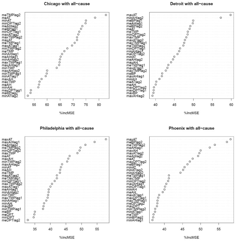
Importance of weather variables in predicting deviation from typical daily total mortality counts as the response variable for four U.S. cities
Note: 1. Importance of weather variables is quantified as the average percent increase in mean squared error; 2. In this analysis, the random forests approach took 20,000 bootstrap samples of summertime (May 1st to September 30th) weather and mortality data from one of four cities, and each sample results in a tree. For each bootstrap sample, mean squared error for a variable was calculated by comparing the predictions from the permuted sample of that variable to those from the unpermuted sample of that variable. A higher average percent increase in mean squared error for a variable suggests that it is more important in predicting outcomes.). 3. This figure shows importance scores of the first 30 variables among all 45 variables. 4. TMP, temperature; DPT, dew point; AT, apparent temperature; STP, barometric pressure; AH, absolute humidity; min, minimum; max, maximum; me, mean; lag 1 or 2, one day or two days before deaths occurred.
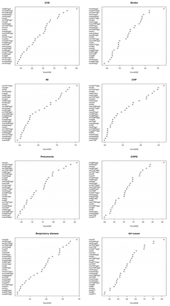
Figure 2-5 show how both the most important variables and the ranking patterns of variables vary with mortality causes and cities. As with all-cause mortality, there were no consistent top variable and exact ranking patterns for each category. Surprisingly, barometric pressure and absolute humidity were much more likely to be selected as the most important variables for seven cause-specific death categories in four cities (12 and 10 times, respectively) than dew point, apparent temperature and temperature (3, 1 and 1 times, respectively). Among the top six variables in 7 cause categories, absolute humidity, barometric pressure, apparent temperature, temperature and dew point appeared 49, 36, 35, 32 and 16 times, respectively.
Figure 2.
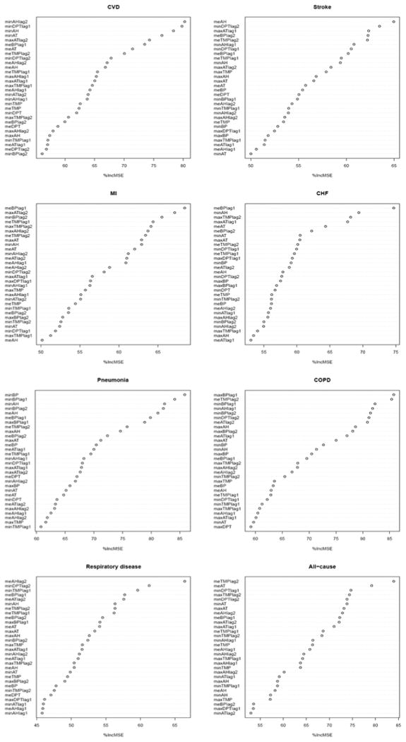
Importance of weather variables in predicting deviation from typical daily cause-specific and all-cause counts as the response variable in Chicago. Otherwise as Figure 1.
Note: CHF, congestive heart failure; COPD, chronic obstructive pulmonary disease; CVD, cardiovascular diseases; MI, myocardial infarction.
Figure 5.
Importance of weather variables in predicting deviation from typical daily cause-specific and all-cause counts as the response variable in Phoenix. Otherwise as Figure 1.
Table S1 shows models generally perform well when outcome variables have relative larger number of daily counts. For example, root mean squared errors of those models for all-cause mortality are within 9 to 14% of mean values of daily counts in four cities. Not surprisingly, model performance varies with city and causes of mortality. Given the same mortality variable, the best model is always identified in Chicago compared to other cities.
Our sensitivity analysis on the degrees of freedom in calculating expected mortality levels shows that the most important variables in four cities are robust to the setting of degrees of freedom. Ranking patterns of variables slightly vary with degrees of freedom.
4. Discussion
The heat epidemiological literature usually uses a single temperature metric or a composition index as a proxy for the complex mixture of weather conditions to which the body is exposed. This study presents a novel multivariate analysis of a mixture of weather conditions and heat-related health effects by applying a robust statistical learning method: the random forests technique. In particular, this analysis ranked the relative importance of each weather condition in predicting the deviations from typical daily mortality counts by modeling 45 weather variables simultaneously within the framework of random forests. Overall, little consistency was observed across cities in the top ranked meteorological variables, or even within city, in the top ranked variables across related causes of death. Given the high degree of correlation in the variables and the low predictive power of temperature for mortality, this may not be surprising. To the extent this is driven by noise in the data, application to a larger number of cities may help resolve which variables are most consistently and strongly associated with mortality.
However, looked at more broadly, a pattern does seem to emerge. Apparent temperature seems the most robust predictor for all-cause mortality across these four cities. Interestingly, absolute humidity, a variable not often included in previous epidemiologic studies, is the second most common predictor for total mortality, and is the most predictive variable for the seven mortality causes, on average. To the best of our knowledge, this study is the first application of random forests in heat exposure and health studies. Random forests are becoming one of the most widely used statistical learning methods because they can deal with a large number of covariates based on a small number of observations, high-order interactions and highly correlated covariates (Strobl et al. 2007). However, the method is rarely applied in environmental sciences and environmental toxicology studies (Coull et al. 2011).
Coull et al. recently applied random forests to assess the associations between pollution mixtures from coal-burning power plants and toxicological endpoints. (Coull et al. 2011) They summarized two advantages and one disadvantage in applying random forests technique to the environmental toxicology field. Their comments are also applicable to the heat-health effects analysis in this paper. Random forests can account for non-linear associations between a covariate and a health outcome. Random forests also relax the assumption of additivity (i.e., the effect of each covariate on an outcome variable is additive) which is commonly assumed in popular statistical methods used in heat-health studies, including multivariate linear regression, generalized linear regression, and generalized additive regression models. This enables us to examine the synergistic effects among either mixtures of weather conditions in this work or mixtures of air pollutants in air pollution epidemiology/toxicology studies. However, unlike the regression methods mentioned earlier, random forests are an algorithm-based statistical method and have the disadvantage of not yielding results that allow for traditional statistical inference (e.g., conducting a hypothesis test, calculating p values or confidence intervals and estimating regression coefficients).
On average, absolute humidity was most frequently selected as one of the top six variables for all-cause mortality and mortality attributable to seven mortality causes used in this analysis. Much of the heat epidemiology literature uses relative humidity as the metric for air moisture, but absolute humidity may be an important metric reflecting physiologically stressful heat exposure. For example, (Shaman and Kohn 2009) point out that absolute humidity can be more relevant biologically for many organisms than relative humidity. In particular, they found that absolute humidity rather than relative humidity is a major driver of influenza seasonality in temperate regions. Relative humidity is calculated as the ratio of the actual amount of moisture in the air (water vapor pressure) compared to the maximum amount of moisture air could hold at a specific temperature (the saturated water vapor pressure). Saturation water vapor pressure increases exponentially with increased temperature, resulting in potentially large differences of absolute moisture given the same relative humidity at different temperatures (Shaman and Kohn, 2009). Absolute humidity is a direct measure of actual moisture in the air, and can be calculated in different ways.
Daily maximum apparent temperature is ranked as the first among all weather variables in the four cities, except for Chicago, and ranks far higher than the second or third most important variable. Apparent temperature and absolute humidity appeared more frequently as one of top six variables compared to other weather parameters. These findings suggest that apparent temperature may be the best proxy to heat exposures in these three cities. Although temperature is ranked as the first in Chicago, the second one is daily mean apparent temperature, which has much higher importance score than the third important variable. Chicago had daily mean temperature at lag 2 ranked as the most important variable, different from other three cities. This might be explained by climate and geographic factors (lake effects in Chicago), socio-demographic status and urban infrastructure, but understanding this difference would require further study.
Several possible reasons why ranking patterns of weather variables vary with cities and mortality causes exist. First, heat-mortality associations are generally small unless they are calculated during heat waves (Barnett et al. 2010), and some uncontrolled factors may change the ranking order, particularly given the correlations among the weather variables. Second, city-specific factors (climate, geographic and population characteristics factors) mentioned earlier may influence these patterns. Third, the underlying mechanisms differ in how heat or heat stress may worsen health among people with pre-existing diseases and may be associated with excess mortality.
The strength of this study is that we used a powerful statistical learning method as a “multi-pollutant” (i.e., ‘multi-weather variable’) tool to assess heat-related health effects. Unlike generalized linear and additive models, this approach can allow for synergistic effects among multiple weather conditions and can handle a large number of highly correlated variables.
This study also has limitations. First, this random forests approach does not produce estimates of relative mortality risk associated with heat like generalized linear or additive models. However, this approach could be used as a screening tool to select which meteorological variables can be incorporated into regression models in providing effect estimates of heat. Second, this study does not include air pollution because our major purpose is to examine which weather conditions are the most important determinants of excess mortality, but future analyses could incorporate pollutants, which influence health and often covary with weather parameters. Third, random forests are a data driven method, and thus the exact ranking patterns may likely change with data set size. However, this probably does not affect our major conclusions which mainly draw on the top six variables rather than the exact ranking patterns.
5. Conclusions
A multivariate analysis was conducted to investigate the synergistic effects of the mixtures of multiple weather variables on heat-related mortality in four US cities using a powerful statistical learning method, random forests. Our investigation showed that, although the importance ranking of weather variables differed by city and mortality causes, apparent temperature appears to be the most robust predictor for all-cause mortality in four cities, and absolute humidity is on average most frequently selected as one of top most predictive important variables for all-cause and cause-specific mortality across four cities. This is a novel finding because absolute humidity could have biological significance for human and some diseases. The analysis and findings presented in this paper are applicable to heat-related epidemiology and toxicology studies, and exposure and risk assessment.
Supplementary Material
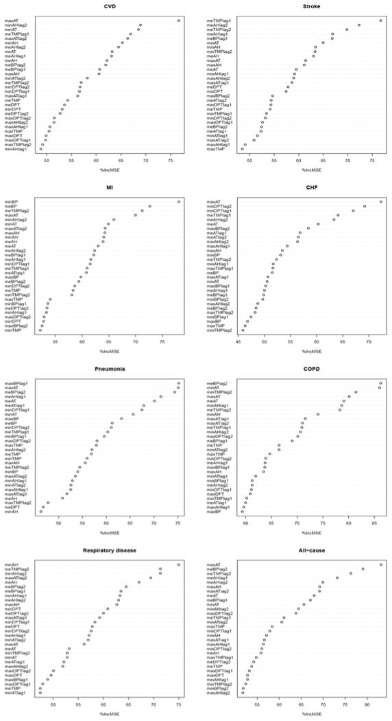
Figure 3.
Importance of weather variables in predicting deviation from typical daily cause-specific and all-cause counts as the response variable in Detroit. Otherwise as Figure 2.
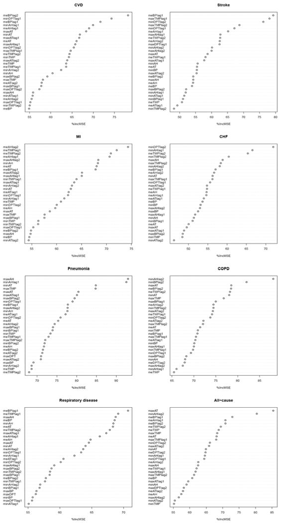
Figure 4.
Importance of weather variables in predicting deviation from typical daily cause-specific and all-cause counts as the response variable in Philadelphia. Otherwise as Figure 1.
Highlights.
Apparent temperature is a robust parameter for activating heat alerts.
Absolute humidity should be included in future heat-health studies.
Random forests can be used to guide choice of weather variables in health studies.
Acknowledgments
The research described in this paper was funded through support of the Graham Environmental Sustainability Institute at the University of Michigan; the U.S. Environmental Protection Agency Science to Achieve Results (STAR) grant R832752010; the U.S. Centers for Disease Control and Prevention grant R18 EH 000348 and National Institute for Environmental Health Sciences grants R01 ES-016932 and R21 ES-020695.
Footnotes
This paper does not necessarily reflect the views of these organizations.
The authors declare they have no competing financial interests.
Publisher's Disclaimer: This is a PDF file of an unedited manuscript that has been accepted for publication. As a service to our customers we are providing this early version of the manuscript. The manuscript will undergo copyediting, typesetting, and review of the resulting proof before it is published in its final citable form. Please note that during the production process errors may be discovered which could affect the content, and all legal disclaimers that apply to the journal pertain.
References
- Barnett AG, Tong S, Clements AC. What measure of temperature is the best predictor of mortality? Environ Research. 2010;110(6):604–611. doi: 10.1016/j.envres.2010.05.006. [DOI] [PubMed] [Google Scholar]
- Bobb JF, Dominici F, Peng RD. A Bayesian model averaging approach for estimating the relative risk of mortality associated with heat waves in 105 U.S. cities. Biometrics. 2011;67(4):1605–16. doi: 10.1111/j.1541-0420.2011.01583.x. [DOI] [PMC free article] [PubMed] [Google Scholar]
- Breiman L. Random forests. Mach Learn. 2001;45(1):5–32. [Google Scholar]
- Coull BA, Wellenius GA, Gonzalez-Flecha B, Diaz E, Koutrakis P, Godleski JJ. The toxicological evaluation of realistic emissions of source aerosols study: Statistical methods. Inhal Toxicol. 2011;23:31–41. doi: 10.3109/08958378.2010.566291. [DOI] [PMC free article] [PubMed] [Google Scholar]
- Faraway JJ. Extending the Linear Model with R: Generalized Linear, Mixed Effects and Nonparametric Regression Models. Boca Raton, FL: Chapman & Hall/CRC; 2006. [Google Scholar]
- Hajat S, Sheridan SC, Allen MJ, Pascal M, Laaidi K, Yagouti A, et al. Heat-health warning systems: A comparison of the predictive capacity of different approaches to identifying dangerously hot days. Am J Public Health. 2010;100(6):1137–44. doi: 10.2105/AJPH.2009.169748. [DOI] [PMC free article] [PubMed] [Google Scholar]
- Hastie T, Tibshirani R, Friedman J. The Elements of Statistical Learning: Data Mining, Inference, and Prediction. Second. New York, NY: Springer Science+Business Media, LLC; 2009. [Google Scholar]
- Klepeis NE, Nelson WC, Ott WR, Robinson JP, Tsang AM, Switzer P, et al. The National Human Activity Pattern Survey (NHAPS): A resource for assessing exposure to environmental pollutants. J Expo Anal Environ Epidemiol. 2001;11(3):231–252. doi: 10.1038/sj.jea.7500165. [DOI] [PubMed] [Google Scholar]
- Kovats RS, Hajat S. Heat stress and public health: A critical review. Annu Rev Public Health. 2007;29:41–55. doi: 10.1146/annurev.publhealth.29.020907.090843. [DOI] [PubMed] [Google Scholar]
- Liaw A, Wiener M. Classification and Regression by randomForest. R News. 2002;2(3):18–22. [Google Scholar]
- Meehl GA, Tebaldi C. More intense, more frequent, and longer lasting heat waves in the 21st century. Science. 2004;305:994–997. doi: 10.1126/science.1098704. [DOI] [PubMed] [Google Scholar]
- Metzger KB, Ito K, Matte TD. Summer heat and mortality in New York City: How hot is too hot? Environ Health Perspect. 2010;118(1):80–86. doi: 10.1289/ehp.0900906. [DOI] [PMC free article] [PubMed] [Google Scholar]
- R Development Core Team. Vienna, Austria: R Foundation for Statistical Computing, Vienna, Austria; 2012. [accessed 5 October 2012]. R: a language and environment for statistical computing. Available: http://www.R-project.org. [Google Scholar]
- Shaman J, Kohn M. Absolute humidity modulates influenza survival, transmission, and seasonality. Proc Natl Acad Sci. 2009;106(9):3243–3248. doi: 10.1073/pnas.0806852106. [DOI] [PMC free article] [PubMed] [Google Scholar]
- Steadman RG. The assessment of sultriness, part I: A temperature humidity index based on human physiology and clothing science. J Appl Meteor. 1979a;18:861–873. [Google Scholar]
- Steadman RG. The assessment of sultriness: Part II: Effects of wind, extra radiation and barometric pressure on apparent temperature. J Appl Meteor. 1979b;18:874–885. [Google Scholar]
- Steadman RG. A universal scale of apparent temperature. J Climate App Meteor. 1984;23:1674–1687. [Google Scholar]
- Strobl C, Boulesteix AL, Zeileis A, Hothorn T. Bias in random forest variable importance measures: Illustrations, sources and a solution. BMC Bioinformatics. 2007;8(1):25. doi: 10.1186/1471-2105-8-25. [DOI] [PMC free article] [PubMed] [Google Scholar]
- Wood SN. Fast stable direct fitting and smoothness selection for generalized additive models. J R Stat Soc Series B Stat Methodol. 2008;70:495–518. [Google Scholar]
- Zanobetti A, Schwartz J. Temperature and mortality in nine US cities. Epidemiology. 2008;19(4):563–570. doi: 10.1097/EDE.0b013e31816d652d. [DOI] [PMC free article] [PubMed] [Google Scholar]
- Zhang K, Rood RB, Michailidis G, Oswald EM, Schwartz JD, Zanobetti A, et al. Comparing exposure metrics for classifying ‘dangerous heat’ in heat wave and health warning systems. Environ Int. 2012;46:23–29. doi: 10.1016/j.envint.2012.05.001. [DOI] [PMC free article] [PubMed] [Google Scholar]
Associated Data
This section collects any data citations, data availability statements, or supplementary materials included in this article.