On the Modeling of Polar Component of Solvation Energy using Smooth Gaussian-Based Dielectric Function

Abstract

Traditional implicit methods for modeling electrostatics in biomolecules use a two-dielectric approach: a biomolecule is assigned low dielectric constant while the water phase is considered as a high dielectric constant medium. However, such an approach treats the biomolecule-water interface as a sharp dielectric border between two homogeneous dielectric media and does not account for inhomogeneous dielectric properties of the macromolecule as well. Recently we reported a new development, a smooth Gaussian-based dielectric function which treats the entire system, the solute and the water phase, as inhomogeneous dielectric medium (J Chem Theory Comput. 2013 Apr 9; 9(4): 2126-2136.). Here we examine various aspects of the modeling of polar solvation energy in such inhomogeneous systems in terms of the solute-water boundary and the inhomogeneity of the solute in the absence of water surrounding. The smooth Gaussian-based dielectric function is implemented in the DelPhi finite-difference program, and therefore the sensitivity of the results with respect to the grid parameters is investigated, and it is shown that the calculated polar solvation energy is almost grid independent. Furthermore, the results are compared with the standard two-media model and it is demonstrated that on average, the standard method overestimates the magnitude of the polar solvation energy by a factor 2.5. Lastly, the possibility of the solute to have local dielectric constant larger than of a bulk water is investigated in a benchmarking test against experimentally determined set of pKa's and it is speculated that side chain rearrangements could result in local dielectric constant larger than 80.

Introduction

Calculations of electrostatic potential and energy of macromolecules are essential to understand the mechanism of biological processes ^1-5. However, these calculations cannot be done analytically for irregularly shaped objects and numerical methods must be applied. The methods can be grouped into two categories, explicit models and implicit models ⁶. Explicit models treat water as individual molecules; in contrast, implicit models average the effect of water phase as continuum media ^7-12. Compared to explicit models, implicit models are more efficient, therefore be able to handle much larger systems ^{10, 13}, however, it comes with the price of losing some atomic information and ambiguity of how to describe the dielectric properties of the system, the solute and the water phases.

A possible solution addressing the above mentioned deficiencies of implicit methods is to develop dielectric function that mimics some of the missing atomic effects. Following the original work of Nicholls and coworkers ¹⁴, recently we reported a smooth Gaussian-based dielectric function implementation in DelPhi ¹⁵. In this implementation, the solute and the water phase are treated on the same footing and there is no sharp dielectric border between them. Even more, the protein surface and protein interior are modeled as an inhomogeneous dielectric medium ¹⁵. While such a model sounds physically more reasonable than the two-dielectric model, it poses the question of how to model the solvation energy. The question has two components: conceptual and technical. The technical question is where to draw the border between solute and the water and the conceptual question is how to treat the solute molecule in absence of the water surrounding.

In the past, the main motivation for introducing Gaussian-based dielectric function was to smooth the boundary solute-water ^{14, 16, 17}. Indeed once the dielectric function distribution is known, the molecular surface can then be defined as surface with a particular value of the dielectric “constant” ^{16, 18, 19}. Typically the optimal value of the dielectric surface is obtained via benchmarking test against experimental data ^20-24. Much less attention was given to the conceptual question of how to treat the solute in absence of water surrounding ²⁵, since such treatment is necessary for the thermodynamics cycle of calculating the polar component of solvation energy (note that the approach of induced surface charges ²⁶ is not straightforward to apply in case of smooth dielectric boundary). In this work we discuss these issues and show their effects on the polar solvation energy calculations.

Another important question which will be addressed in this work is the upper bound of the dielectric “constant” inside a biomolecule. Previous work of Zhou and coworkers ²² using zero probe radius to deliver the molecular surface and dielectric map within a Poisson-Boltzmann solver showed that such an approach results not only in different molecular surface (vdW surface), but also introduces many cavities inside the molecule ²⁷. These cavities were considered high dielectric cavities with dielectric constant of 80 (bulk water), and it was reasoned by the experimental observation that water molecules can propagate inside biomolecules ^{28, 29}. However, we argue that the water penetration may not be the only and the most important contributor to the high local dielectric constant inside biomolecules. Reorientation of charged side chains or structural changes associated with charged domains may have a larger effect on the dielectric properties of the macromolecule than water penetration, and may result effective local dielectric constant larger than 80.

Since the solutions are provided via a grid algorithm, the finite-difference method ³⁰, implemented in DelPhi ^{11, 31}, is desirable for probing how sensitive the results are with respect to the parameters of the grid; especially the grid spacing, frequently termed “scale”. It is anticipated that at fine grid spacing (larger scale), the solutions will be more reliable, however, one wants to achieve such reliable solutions at smallest computational cost in terms of time and memory. Here we test the scale convergence of the solutions delivered with the smooth Gaussian-based function and compare with the convergence of the solutions obtained with induced surface charges method. The motivation for such comparison stems from the fact that in the two-dielectric model, it was repeatedly shown that the induced charges method outperforms the standard method of calculating the polar solvation energy and is almost grid independent at grid resolution larger than 1Å/grid ¹¹.

Method

1. Smooth Gaussian-based dielectric function

The smooth Gaussian-based dielectric function was previously described ¹⁵, therefore here it will be only briefly outlined. Following Nicholls and coworkers ¹⁴, the atomic density at position r generated by atom i is calculated as:

$${\rho }_i(r)=exp[-r_i^2/({\sigma }^2\cdot R_i^2)],$$ (1)

where ρ_i (r) is atomic density at position r generated by atom i; r_i is distance between r and center of atom i; σ² is the variance of Gaussian distribution; R_i is the radius of atom i defined by force filed used.

Then, the total atomic density is calculated as:

$${\rho }_{\mathit{\text{mol}}}(r)=1-\prod _i[1-{\rho }_i(r)],$$ (2)

where ρ_mol (r) is the is total atomic density at position r generated by the whole molecule; ρ_i (r) is atomic density generated by atom i. This equation guarantees that the total atomic density at the atom-atom overlapping region is higher than in each of the single atom, but the total density will not exceeds 1.

Finally, the atomic density is converted into a dielectric distribution as:

$$\epsilon (r)={\rho }_{\mathit{\text{mol}}}(r)\cdot {\epsilon }_{\mathit{\text{in}}}+(1-{\rho }_{\mathit{\text{mol}}}(r))\cdot {\epsilon }_{\mathit{\text{out}}}$$ (3)

here ε(r) is dielectric distribution of the molecule. ε_in is the reference dielectric value for biomolecules, ε_out is the dielectric value for water.

2. Calculating polar component of solvation energy

Currently DelPhi calculates the polar solvation energy in the case of sharp dielectric border(s) via the induced surface charges (reaction field energy) subroutine, an approach which was repeatedly shown to outperform the standard two steps methods ²⁶. However, the implementation of a similar approach in the case of smooth dielectric boundary would require integration over the transition layer of solute-bulk water. Currently this is computationally inefficient, and because of that the two steps procedure was implemented.

This standard two steps method is implemented as follow: 1. A 3D dielectric distribution is calculated by using equation (1)-(3), and the grid energy G_{protein–water} of the system is calculated. 2. A Gaussian “surface” is constructed by selecting a certain epsilon value (such as epsilon=20). The epsilon values outside the surface are then set to have the value of vacuum, while the epsilon distribution inside the surface stays the same as in step 1. The motivation for this is assumption at in vacuum the protein retains its properties. Then the grid energy of this new system is calculated as G_{protein–vacuum}. The difference between the grid energies in the above two steps is the solvation energy.

$$G_{\mathit{\text{solvation}}}=G_{\mathit{\text{protein}}–\mathit{\text{vacuum}}}-G_{\mathit{\text{protein}}–\mathit{\text{water}}}$$ (4)

3. Structure files and parameters used in the calculations

The calculations were performed on a protein data set of 91 proteins ¹⁵. The selection of these 91 files was previously described ¹⁵. These structures were used to carry out calculations for the polar component of the solvation energy. In the case of smooth Gaussian-based dielectric function, the reference dielectric value ε_in was set to be 4.0, and the variance σ was 0.93. These two parameters were optimized in our previous test on pKa calculations ¹⁵. The epsilon for surface cutoff is set to be =20, which is optimized from small molecule test ¹⁵. For the other parameters, perfil is set as 70, salt concentration is 0, the scale is set as 2.0. The force field used is Amber ³².

4. Scale/resolution dependence

To investigate the sensitivity of the results with respect to the grid resolution (scale), the following considerations were made: since the test cases are real proteins for which polar solvation energy cannot be calculate analytically, one needs to define what the correct energy is. It is well known that an increase of the resolution (larger scale) would result in more accurate results. Because of that, the following measure of the accuracy was adopted:

$$G_i^{\mathit{\text{error}}}=\frac{|G_{\mathit{\text{scale}}=i}-G_{\mathit{\text{scale}}=6.0}|}{\left|G_{\mathit{\text{scale}}=6.0}\right|}$$ (5)

where $G_i^{\mathit{\text{error}}}$ is the scale relative error at scale= i, G_scale=6.0 is the reference grid energy, which is considered to be the correct energy. For each protein in the dataset $G_i^{\mathit{\text{error}}}$ is calculated and the scale i was varied from 0.2 to 6.0 with step= 0.2.

5. Upper bound of dielectric constant inside biomolecule

In the original equation (3), the upper bound of the dielectric constant of a biomolecule is the same as the dielectric constant value of water ε_out. This is because the original model attempts to account for water penetration inside the biomolecule only. However, we argue that side chain rearrangement and structural domains motion may cause even larger dielectric effect than water penetration. Such a possibility is illustrated in the supplementary material by a simplified example (figure S1). To allow the local dielectric constant inside the biomolecule to sample values larger than those of bulk water, the equation (3) is modified as:

$$\epsilon =\{\begin{array}{cc}{\epsilon }_{\mathit{\text{out}}},& \text{when}\rho =0\\ \rho \cdot {\epsilon }_{\mathit{\text{in}}}+(1-\rho )\cdot {\epsilon }_{\mathit{\text{out}}}^{\prime },& \text{when}\rho >0\end{array}$$ (6)

where ε is the dielectric value for the entire biomolecule-water system. ρ is the atomic density of the system. ρ equal to 0 means the region is totally in water, in this case the dielectric is set as ε_out, which is 80; when ρ > 0, or inside the biomolecule, the upper bound of dielectric constant is set as ε′_out, which can be bigger than 80.

Results and discussions

1. Comparing polar solvation energy calculated with smooth Gaussian-based dielectric function and the standard two-dielectric model

The vast majority of the polar solvation energy calculations reported in literature were done with the two-dielectric model ^33-36, while only a few cases considered that the protein may have structural regions with different dielectric properties ^{25, 37, 38}. However, in all cases the boundary between different dielectric regions inside the biomolecule (and in most of cases between solute and water) was considered to have sharp borders. Since our approach differs from these cases, it will be useful to investigate how the calculated polar solvation energies compare among the models.

To carry out such an investigation, the polar solvation energies were calculated using both the two-dielectric homogeneous model and the smooth Gaussian-based dielectric function, both available in DelPhi distribution ¹¹, on the dataset of 91 proteins ¹⁵. The parameters for the calculations utilizing the smooth Gaussian-based dielectric function were provided in the method section (ε_in = 4.0 and σ = 0.93), while the internal dielectric constant ε_in for the two-dielectric model was varied from 2.0 to 12.0 in steps of 2.0. Then, the polar solvation energies obtained with two-dielectric model (homogeneous internal dielectric constant, termed “Homo” for short; ΔG_Homo) and with smooth Gaussian-based dielectric function (termed “Gaussian”; ΔG_Gaussian) were compared via linear regression:

$$\mathrm{\Delta }{G}_{\mathit{\text{Homo}}}=a\mathrm{\Delta }{G}_{\mathit{\text{Gaussian}}}+b$$ (7)

For each ε_in of homogeneous method, a and b are determined by the linear regression method. Moreover, the correlation between ΔG_Homo and ΔG_Gaussian is also calculated (Figure S2 and Table 1).

Table 1.

Comparison between ΔG_Gaussian and ΔG_Homo with different ε_in.

εin	correlation	a	b(kT)
2	0.951	5.9747	-312.5323
4	0.953	2.8726	-147.744
6	0.955	1.8428	-93.1143
8	0.957	1.3304	-66.0189
10	0.959	1.0245	-49.9243
12	0.960	0.8217	-39.3187

In this table 1, parameters for Gaussian method are fixed: ε_in = 4.0 and σ = 0.93; For each ε_in of homogeneous method, the correlation between ΔG_Homo and ΔG_Gaussian is calculated, a and b are determined by the linear regression method.

In analyzing the results from figure S1 (see Supporting Information), one can appreciate that the points are scattered along the main diagonal, the largest deviations observed for cases with large polar solvation energies. The pattern does not change as ε_in varies from 2.0 to 12.0 in the two-dielectric model, but the slope of the fitting line does. Despite the irregular shape of the proteins used in the dataset, still such a behavior is expected based on the Born solvation model ³⁹. The best correspondence between results calculated with the smooth Gaussian-based dielectric function and two-dielectric model are obtained with ε_in =10.0 (for the internal dielectric constant in two-dielectric model). Such a correspondence was also found in pKa calculations from our previous work ¹⁵. The correlation coefficient between the Gaussian method and the homogeneous method with ε_in =10.0 is P=0.959; the slope a is 1.02 and b is -49.92 kT. From table 1, the slopes change against ε_in, when ε_in =10, the slope a is very close to 1.0. However, even when ε_in =10, the correlation is still 0.959 and b is -49.92kT. This indicates that when ε_in =10, the solvation energies calculated by homogeneous method and Gaussian method have very similar tendency, but the two methods do have differences for individual proteins. Actually the differences for individual proteins are expected, this is the reason why the Gaussian method was able to obtain better results on pKa and some other calculations ¹⁵.

2. Scale dependence

Scale dependence is an important feature for PB solvers implemented in the finite difference method^{40, 41}. In previous work, we demonstrated that the Gaussian method performs better on grid shift error and rotation error compared to the homogeneous method ¹⁵. In this work, we tested the scale dependence error using equation (5). Figure 2 shows the results of scale error for the Gaussian method and the homogeneous method. It is important to note that in the homogeneous method, the traditional two-step method was replaced by an induced charges method for solvation energy calculation ²⁶. This induced charges method has been proved to be less scale dependent than the two-step method ²⁶. In this work, the comparison is between the homogeneous method with induced charge method and the Gaussian method with the two steps method (as it was mentioned above, a straightforward implementation of the induced charges method in the smooth Gaussian-based dielectric model is currently computationally demanding).

Figure 2.

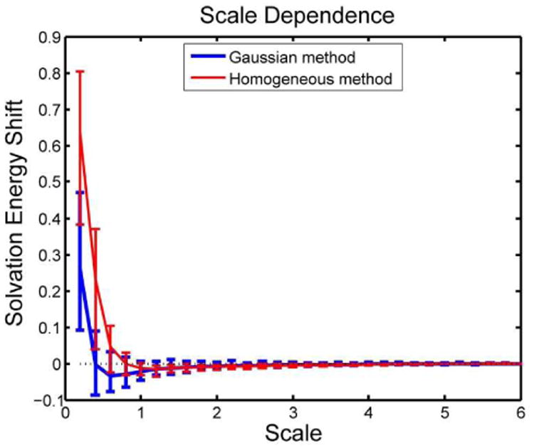
Scale dependence comparison between homogeneous and Gaussian methods on solvation calculations.

Figure 2 shows that at scale=2.0 grid/Å (resolution 0.5 Å/grid), both methods are able to obtain results with scale error < 1%, but the smooth Gaussian-based dielectric function yields better accuracy (scale error <0.8%). The standard deviations are quite similar. However, at scale < 2grids/Å (worsened resolution), the smooth Gaussian-based dielectric function outperforms the two-dielectric model in both the scale error and standard deviation.

What is the reason for the smooth Gaussian-based dielectric method to outperform the two-dielectric method even though it utilizes a less accurate approach (in terms of the grid algorithm) in polar solvation energy calculations? Figure 3 is a cartoon presentation of mapping of a single atom onto the grid and is aimed to offer an explanation of the observed effect. It can be seen that the same atom is represented in quite different ways by the homogeneous and the Gaussian method. In this figure, red lines are epsilon distributions under low scale, blue lines are epsilon distribution under high scale. 1. Homogenous method results sharp epsilon jump near the boundary, no matter how large the scale is used; in contrast, Gaussian model always generates smoother epsilon distribution. When the scale is larger, the epsilon distribution generated by Gaussian model is even smoother. 2. From figure 3 e, one can see that when different scales are used to model the same atom in the homogeneous method, the epsilon distributions could be very different, which results a difference of born radius of this single atom and generates the scale error; however, when scales are different, the epsilon distributions of the Gaussian method are more similar to each other. These two factors are the main reasons which cause the Gaussian method to be less scale dependent than the homogeneous method.

Figure 3.

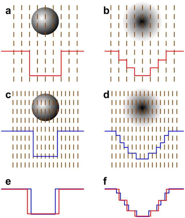
Illustration for scale dependence feature of homogenous method and Gaussian method. a. one-dimensional epsilon distribution in homogeneous method with a low scale. b. one-dimensional epsilon distribution in Gaussian method with a low scale. c. Epsilon distribution in the homogeneous method with a high scale. d. Epsilon distribution in the Gaussian method with a high scale. e. Comparison of epsilon distributions using low and high scales for the same system in the homogeneous method. f. Comparison of epsilon distributions using low and high scales for the same system in the Gaussian method.

3. Upper bound of dielectric constant

Side chain rearrangement affects the dielectric property of biomolecules. If the side chain flexibility is considered (figure S1), the upper bound of the dielectric constant of the biomolecule could be even higher than epsilon for water. Supporting Information (figure S1) offers a simple example illustrating that charged side chain rearrangement can generate local electrostatic field larger than the local electrostatic field generated by water reorientation. Therefore, in principle, the internal dielectric constant of biomolecules could be larger than of the bulk water.

Here we explore the possibility of assigning local internal dielectric constant larger than 80 in a benchmarking test against experimentally determined pKa's taken from pKa-cooperative ^{42, 43} (http://pkacoop.org/wordpress/?p=28). It should be emphasized that these pKa values are highly perturbed resulting in pKa shifts of 5 and more units. Previous continuum electrostatic based pKa calculations showed that the value of internal dielectric constant has prominent effect of the calculated pKa shifts ⁴⁴. It was pointed out that larger internal dielectric constant results in smaller pKa shifts ⁴⁴. Since the experimental dataset is comprised of cases with large pKa shifts, it is anticipated that further rising of the internal dielectric constant above the optimal value for a given model should result worsen pKa shifts predictions. In our previous work ¹⁵, the upper bound of dielectric constant for the Gaussian method was set as 80. Here we carry the same type of calculations, but allow the local internal dielectric constant to sample values larger than 80. Thus, the parameters of the smooth Gaussian-based dielectric function are the same as in the previous work ¹⁵, with the only difference that the ε′_out varies as 100, 120 and 60. The results are summarized in Table 2.

Table 2.

Top 20 results in terms of the RMSD between calculated and experimental pKa shift.

Eps(in)	sigma	Eps'(out)	RMSD
8.0	1.00	120	1.69
8.0	0.99	120	1.70
8.0	1.00	100	1.71
6.0	0.96	120	1.72
8.0	1.01	120	1.72
6.0	0.97	120	1.72
6.0	0.97	100	1.72
8.0	1.01	100	1.73
4.0	0.93	120	1.73
6.0	0.96	100	1.73
4.0	0.93	100	1.73
8.0	0.99	100	1.73
8.0	0.98	120	1.74
4.0	0.94	100	1.74
4.0	0.94	120	1.75
6.0	0.95	120	1.76
8.0	1.02	100	1.77
6.0	0.98	100	1.77

Table 2 shows the best 20 results in terms of the RMSD between calculated and experimental pKa shift along with the corresponding parameters of the protocol. All of these RMSDs are smaller than in the previous work, which was 1.77, indicating better performance. In all top 20 results, the ε′_out value is always larger than 80. This indicates that by increasing the value of upper bound of the dielectric value inside biomolecule, the calculations result in better predicted pKa shifts. Interestingly, the increase of the upper bound of the internal dielectric constant did not result in change of neither the reference dielectric constant nor the variance in the Gaussian formula. Indeed, when ε_in is 4.0, the best σ value is still 0.93, in accordance with our previous results. At the same time, the optimal upper bound of the internal dielectric constant ε′_out is now 120, rather than 80. These results indicate that perhaps the side chain and domain rearrangements occurring in the pKa experiments can be better modeled via dielectric function which can take local values larger than of 80. For illustration figure S3 (in Supporting Information) shows the distribution of the dielectric constant with upper bound of 80 and 120. It can be seen that the change of the upper bound affects not only the surface regions, but also some regions inside the biomolecule.

Conclusion

The scale dependence of the results is one of the most critical drawbacks of finite difference methods. It forces researchers to perform calculations at various scales (resolutions) to test the sensitivity of the results and to use fine scales which results in computationally demanding simulations. To avoid this drawback, the standard homogenous algorithm implemented in DelPhi uses the method of induced surface changes to calculate solvation energy. However, in the case of the Gaussian-based smooth dielectric function, this method cannot be easily applied and the concern was that the smoothed dielectric boundary may result is worsening the grid dependence of the solvation energy calculations. However, the results reported in the paper clearly indicate that this is not the case and that the smooth Gaussian-based dielectric function performs even better than the induced surface charges algorithm. This observation is attributed to the lesser sensitivity of the region solute-water mapping onto the grid as compared with the sharp boundary mapping. Less scale dependence is an inherent feature of the smooth Gaussian-based dielectric distribution.

The protein interior in water phase and in vacuum was modeled with the same dielectric distribution, an important detail of the reported approach. This is justified by the observation that frequently protein molecules retain their structures and functions when transferred in gas phase ^45-48. Because of that, their intrinsic flexibility and therefore dielectric properties in vacuum should remain the same as in water phase.

Since so far, almost all reported modelings of the solvation energy are done with the standard two-dielectric model, one may wonder what the approximate correspondence is with respect to the calculations done with the smooth Gaussian-based dielectric function. It was found that the rough correspondence is 2.5, i.e. the two-dielectric model overestimates the solvation energy by factor of 2.5. However, this observation should be taken with caution since the individual energies could be different by more than several tens of kTs. This indicates that the smooth Gaussian-based model cannot be replaced by the homogeneous model in the way of selecting “proper” dielectric constant, because no matter what dielectric constant value is used, the dielectric distribution of homogeneous model will always lose some atomic details, on the contrast, the smooth Gaussian-based method reflects some of the atomic details of the solute and water phase.

Previous works considered the possibility that the dielectric constant of solute may be a large number ^33-36. Such a possibility was attributed to plausible water penetration inside the solute and therefore the upper bound of dielectric constant inside molecules was considered to be 80. However, the side chains or entire structural domains may be quite flexible and may be charged. Considering the effect of such flexible charges, the upper bound of dielectric constant inside molecules could be even higher than 80. In this work, it is found that by increasing the upper bound of the dielectric constant of biomolecules, we can obtain even more accurate pKa calculations as compared with the case of using 80 for the upper bound of internal dielectric constant.

Figure 1.

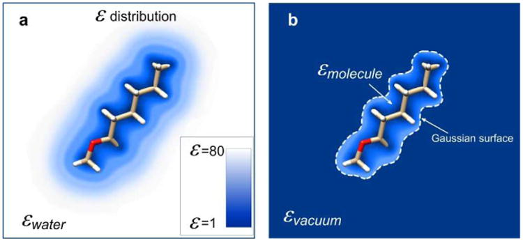
The standard two-step method for solvation energy calculations. The left panel shows the solute in water phase and the levels of the dielectric constant values are color-coded. The right panel illustrates the same solute in vacuum. Note that the dielectric constant distribution inside the molecular surface is identical to the dielectric constant distribution in water.

References

- 1.Warshel A, Papazyan A. Electrostatic effects in macromolecules: fundamental concepts and practical modeling. Current Opinion in Structural Biology. 1998;8(2):211–217. doi: 10.1016/s0959-440x(98)80041-9. [DOI] [PubMed] [Google Scholar]
- 2.Zhang Z, Witham S, Alexov E. On the role of electrostatics in protein–protein interactions. Physical biology. 2011;8(3):035001. doi: 10.1088/1478-3975/8/3/035001. [DOI] [PMC free article] [PubMed] [Google Scholar]
- 3.Ren P, Chun J, Thomas DG, Schnieders MJ, Marucho M, Zhang J, Baker NA. Biomolecular electrostatics and solvation: a computational perspective. Quarterly reviews of biophysics. 2012;45(04):427–491. doi: 10.1017/S003358351200011X. [DOI] [PMC free article] [PubMed] [Google Scholar]
- 4.Boehr DD, Nussinov R, Wright PE. The role of dynamic conformational ensembles in biomolecular recognition. Nature chemical biology. 2009;5(11):789–796. doi: 10.1038/nchembio.232. [DOI] [PMC free article] [PubMed] [Google Scholar]
- 5.Onufriev AV, Alexov E. Protonation and pK changes in protein–ligand binding. Quarterly reviews of biophysics. 2013;46(02):181–209. doi: 10.1017/S0033583513000024. [DOI] [PMC free article] [PubMed] [Google Scholar]
- 6.Li C, Li L, Petukh M, Alexov E. Progress in developing Poisson-Boltzmann equation solvers. Molecular Based Mathematical Biology. 2013;1:42–62. doi: 10.2478/mlbmb-2013-0002. [DOI] [PMC free article] [PubMed] [Google Scholar]
- 7.Chen Z, Zhao S, Chun J, Thomas DG, Baker NA, Bates PW, Wei G. Variational approach for nonpolar solvation analysis. The Journal of Chemical Physics. 2012;137:084101. doi: 10.1063/1.4745084. [DOI] [PMC free article] [PubMed] [Google Scholar]
- 8.Botello-Smith WM, Liu X, Cai Q, Li Z, Zhao H, Luo R. Numerical Poisson-Boltzmann model for continuum membrane systems. Chemical physics letters. 2012 doi: 10.1016/j.cplett.2012.10.081. [DOI] [PMC free article] [PubMed] [Google Scholar]
- 9.Che J, Dzubiella J, Li B, McCammon JA. Electrostatic free energy and its variations in implicit solvent models. The Journal of Physical Chemistry B. 2008;112(10):3058–3069. doi: 10.1021/jp7101012. [DOI] [PubMed] [Google Scholar]
- 10.Baker NA, Sept D, Joseph S, Holst MJ, McCammon JA. Electrostatics of nanosystems: application to microtubules and the ribosome. Proceedings of the National Academy of Sciences. 2001;98(18):10037–10041. doi: 10.1073/pnas.181342398. [DOI] [PMC free article] [PubMed] [Google Scholar]
- 11.Li L, Li C, Sarkar S, Zhang J, Witham S, Zhang Z, Wang L, Smith N, Petukh M, Alexov E. DelPhi: a comprehensive suite for DelPhi software and associated resources. BMC biophysics. 2012;5(1):9. doi: 10.1186/2046-1682-5-9. [DOI] [PMC free article] [PubMed] [Google Scholar]
- 12.Harris RC, Mackoy T, Fenley MO. A Stochastic Solver of the Generalized Born Model. Molecular Based Mathematical Biology. 2013;1:63–74. [Google Scholar]
- 13.Li C, Li L, Zhang J, Alexov E. Highly efficient and exact method for parallelization of grid - based algorithms and its implementation in DelPhi. Journal of Computational Chemistry. 2012;33(24):1960–1966. doi: 10.1002/jcc.23033. [DOI] [PMC free article] [PubMed] [Google Scholar]
- 14.Grant JA, Pickup BT, Nicholls A. A smooth permittivity function for Poisson–Boltzmann solvation methods. Journal of Computational Chemistry. 2001;22(6):608–640. [Google Scholar]
- 15.Li L, Li C, Zhang Z, Alexov E. On the Dielectric “Constant” of Proteins: Smooth Dielectric Function for Macromolecular Modeling and Its Implementation in DelPhi. Journal of chemical theory and computation. 2013;9(4):2126–2136. doi: 10.1021/ct400065j. [DOI] [PMC free article] [PubMed] [Google Scholar]
- 16.Im W, Beglov D, Roux B. Continuum solvation model: computation of electrostatic forces from numerical solutions to the Poisson-Boltzmann equation. Computer Physics Communications. 1998;111(1):59–75. [Google Scholar]
- 17.Word JM, Nicholls A. Application of the Gaussian dielectric boundary in Zap to the prediction of protein pKa values. Proteins: Structure, Function, and Bioinformatics. 2011;79(12):3400–3409. doi: 10.1002/prot.23079. [DOI] [PubMed] [Google Scholar]
- 18.Blinn JF. A generalization of algebraic surface drawing. ACM Transactions on Graphics (TOG) 1982;1(3):235–256. [Google Scholar]
- 19.Zhang Y, Xu G, Bajaj C. Quality meshing of implicit solvation models of biomolecular structures. Computer Aided Geometric Design. 2006;23(6):510–530. doi: 10.1016/j.cagd.2006.01.008. [DOI] [PMC free article] [PubMed] [Google Scholar]
- 20.Lee B, Richards FM. The interpretation of protein structures: estimation of static accessibility. Journal of molecular biology. 1971;55(3):379–IN4. doi: 10.1016/0022-2836(71)90324-x. [DOI] [PubMed] [Google Scholar]
- 21.Connolly ML. Analytical molecular surface calculation. Journal of Applied Crystallography. 1983;16(5):548–558. [Google Scholar]
- 22.Pang X, Zhou HX. Poisson-Boltzmann Calculations: van der Waals or Molecular Surface? Commun Comput Phys. 2013;13:1–12. doi: 10.4208/cicp.270711.140911s. [DOI] [PMC free article] [PubMed] [Google Scholar]
- 23.Grant JA, Pickup B. A Gaussian description of molecular shape. The Journal of Physical Chemistry. 1995;99(11):3503–3510. [Google Scholar]
- 24.Chen Z, Baker NA, Wei GW. Differential geometry based solvation model I: Eulerian formulation. Journal of computational physics. 2010;229(22):8231–8258. doi: 10.1016/j.jcp.2010.06.036. [DOI] [PMC free article] [PubMed] [Google Scholar]
- 25.Wang L, Zhang Z, Rocchia W, Alexov E. Using DelPhi Capabilities to Mimic Protein's Conformational Reorganization with Amino Acid Specific Dielectric Constants. Comm Comp Phys. 2012 doi: 10.4208/cicp.300611.120911s. [DOI] [PMC free article] [PubMed] [Google Scholar]
- 26.Rocchia W, Sridharan S, Nicholls A, Alexov E, Chiabrera A, Honig B. Rapid grid - based construction of the molecular surface and the use of induced surface charge to calculate reaction field energies: Applications to the molecular systems and geometric objects. Journal of Computational Chemistry. 2002;23(1):128–137. doi: 10.1002/jcc.1161. [DOI] [PubMed] [Google Scholar]
- 27.Alexov E. Role of the protein side - chain fluctuations on the strength of pair - wise electrostatic interactions: Comparing experimental with computed pKas. Proteins: Structure, Function, and Bioinformatics. 2003;50(1):94–103. doi: 10.1002/prot.10265. [DOI] [PubMed] [Google Scholar]
- 28.Vaitheeswaran S, Yin H, Rasaiah JC, Hummer G. Water clusters in nonpolar cavities. Proceedings of the National Academy of Sciences of the United States of America. 2004;101(49):17002–17005. doi: 10.1073/pnas.0407968101. [DOI] [PMC free article] [PubMed] [Google Scholar]
- 29.Yin H, Feng G, Clore GM, Hummer G, Rasaiah JC. Water in the Polar and Nonpolar Cavities of the Protein Interleukin-1β†. The Journal of Physical Chemistry B. 2010;114(49):16290–16297. doi: 10.1021/jp108731r. [DOI] [PMC free article] [PubMed] [Google Scholar]
- 30.Klapper I, Hagstrom R, Fine R, Sharp K, Honig B. Focusing of electric fields in the active site of Cu - Zn superoxide dismutase: Effects of ionic strength and amino - acid modification. Proteins: Structure, Function, and Bioinformatics. 1986;1(1):47–59. doi: 10.1002/prot.340010109. [DOI] [PubMed] [Google Scholar]
- 31.Nicholls A, Honig B. A rapid finite difference algorithm, utilizing successive over - relaxation to solve the Poisson–Boltzmann equation. Journal of Computational Chemistry. 1991;12(4):435–445. [Google Scholar]
- 32.Ponder JW, Case DA. Force fields for protein simulations. Advances in protein chemistry. 2003;66:27–85. doi: 10.1016/s0065-3233(03)66002-x. [DOI] [PubMed] [Google Scholar]
- 33.Gunner M, Zhu X, Klein MC. MCCE analysis of the pKas of introduced buried acids and bases in staphylococcal nuclease. Proteins: Structure, Function, and Bioinformatics. 2011;79(12):3306–3319. doi: 10.1002/prot.23124. [DOI] [PubMed] [Google Scholar]
- 34.Warwicker J. pKa predictions with a coupled finite difference Poisson–Boltzmann and Debye–Hückel method. Proteins: Structure, Function, and Bioinformatics. 2011;79(12):3374–3380. doi: 10.1002/prot.23078. [DOI] [PubMed] [Google Scholar]
- 35.Spassov VZ, Yan L. A fast and accurate computational approach to protein ionization. Protein Science. 2008;17(11):1955–1970. doi: 10.1110/ps.036335.108. [DOI] [PMC free article] [PubMed] [Google Scholar]
- 36.Antosiewicz J, McCammon JA, Gilson MK. Prediction of pH-dependent properties of proteins. Journal of molecular biology. 1994;238(3):415–436. doi: 10.1006/jmbi.1994.1301. [DOI] [PubMed] [Google Scholar]
- 37.Alexov E, Gunner M. Calculated protein and proton motions coupled to electron transfer: electron transfer from QA-to QB in bacterial photosynthetic reaction centers. Biochemistry. 1999;38(26):8253–8270. doi: 10.1021/bi982700a. [DOI] [PubMed] [Google Scholar]
- 38.Rocchia W, Alexov E, Honig B. Extending the applicability of the nonlinear Poisson-Boltzmann equation: Multiple dielectric constants and multivalent ions. The Journal of Physical Chemistry B. 2001;105(28):6507–6514. [Google Scholar]
- 39.Bashford D, Case DA. Generalized Born models of macromolecular solvation effects. Annual Review of Physical Chemistry. 2000;51(1):129–152. doi: 10.1146/annurev.physchem.51.1.129. [DOI] [PubMed] [Google Scholar]
- 40.Harris RC, Boschitsch AH, Fenley MO. Influence of Grid Spacing in Poisson-Boltzmann Equation Binding Energy Estimation. Journal of chemical theory and computation. 2013 doi: 10.1021/ct300765w. [DOI] [PMC free article] [PubMed] [Google Scholar]
- 41.Wang J, Cai Q, Xiang Y, Luo R. Reducing Grid Dependence in Finite-Difference Poisson–Boltzmann Calculations. Journal of chemical theory and computation. 2012;8(8):2741–2751. doi: 10.1021/ct300341d. [DOI] [PMC free article] [PubMed] [Google Scholar]
- 42.Pey AL, Rodriguez-Larrea D, Gavira JA, Garcia-Moreno B, Sanchez-Ruiz JM. Modulation of buried ionizable groups in proteins with engineered surface charge. Journal of the American Chemical Society. 2010;132(4):1218–1219. doi: 10.1021/ja909298v. [DOI] [PubMed] [Google Scholar]
- 43.Isom DG, Cannon BR, Castañeda CA, Robinson A. High tolerance for ionizable residues in the hydrophobic interior of proteins. Proceedings of the National Academy of Sciences. 2008;105(46):17784–17788. doi: 10.1073/pnas.0805113105. [DOI] [PMC free article] [PubMed] [Google Scholar]
- 44.Alexov E, Mehler EL, Baker N, Baptista AM, Huang Y, Milletti F, Erik Nielsen J, Farrell D, Carstensen T, Olsson MH. Progress in the prediction of pKa values in proteins. Proteins: Structure, Function, and Bioinformatics. 2011;79(12):3260–3275. doi: 10.1002/prot.23189. [DOI] [PMC free article] [PubMed] [Google Scholar]
- 45.Shelimov KB, Jarrold MF. Conformations, unfolding, and refolding of apomyoglobin in vacuum: An activation barrier for gas-phase protein folding. Journal of the American Chemical Society. 1997;119(13):2987–2994. [Google Scholar]
- 46.van der Spoel D, Marklund EG, Larsson DS, Caleman C. Proteins, lipids, and water in the gas phase. Macromolecular bioscience. 2011;11(1):50–59. doi: 10.1002/mabi.201000291. [DOI] [PubMed] [Google Scholar]
- 47.Deng L, Broom A, Kitova EN, Richards MR, Zheng RB, Shoemaker GK, Meiering EM, Klassen JS. Kinetic stability of the streptavidin–biotin interaction enhanced in the gas phase. Journal of the American Chemical Society. 2012;134(40):16586–16596. doi: 10.1021/ja305213z. [DOI] [PubMed] [Google Scholar]
- 48.Hopper JT, Rawlings A, Afonso JP, Channing D, Layfield R, Oldham NJ. Evidence for the preservation of native inter-and intra-molecular hydrogen bonds in the desolvated FK-binding protein· FK506 complex produced by electrospray ionization. Journal of The American Society for Mass Spectrometry. 2012;23(10):1757–1767. doi: 10.1007/s13361-012-0430-y. [DOI] [PubMed] [Google Scholar]
Associated Data
This section collects any data citations, data availability statements, or supplementary materials included in this article.