Relative Binding Enthalpies from Molecular Dynamics Simulations Using a Direct Method

Abstract

The potential for reliably predicting relative binding enthalpies, ΔΔE, from a direct method utilizing molecular dynamics is examined for a system of three phosphotyrosyl peptides binding to a protein receptor, the Src SH2 domain. The binding enthalpies were calculated from the potential energy differences between the bound and the unbound end-states of each peptide from equilibrium simulations in explicit water. The statistical uncertainties in the ensemble-mean energy values from multiple, independent simulations were obtained using a bootstrap method. Simulations were initiated with different starting coordinates as well as different velocities. Statistical uncertainties in ΔΔE are 2 to 3 kcal/mol based on calculations from 40, 10 ns trajectories for each system (three SH2–peptide complexes or unbound peptides). Uncertainties in relative component energies, comprising solute–solute, solute–solvent and solvent–solvent interactions, are considerably larger. Energy values were estimated from an unweighted ensemble averaging of multiple trajectories with the a priori assumption that all trajectories are equally likely. Distributions in energy–rmsd space indicate that the trajectories sample the same basin and the difference in mean energy values between trajectories is due to sampling of alternative local regions of this superbasin. The direct estimate of relative binding enthalpies is concluded to be a reasonable approach for well-ordered systems with ΔΔE values greater than ∼3 kcal/mol, although the approach would benefit from future work to determine properly distributed starting points that would enable efficient sampling of conformational space using multiple trajectories.

Introduction

The rapid growth in computational capabilities enables the use of computer simulations to help guide our understanding of biomolecules and their interactions at a level previously unrealized. Estimation of thermodynamic quantities by simulation is particularly important to gain insight into the microscopic details and connect physical interactions with thermodynamic measurements. Here, we consider the direct calculation from molecular dynamics (MD) simulation of the binding enthalpy for a protein–peptide complex. A description of how changes in ligand structure perturb molecular interactions, and hence enthalpy, can provide insight into enthalpy–entropy compensation, or help to explain subtle effects on binding energy when these are difficult to resolve based on crystallographic or NMR structures.^1,2 Furthermore, a strategy to improve the affinity of drug candidates is based on optimizing binding enthalpy and entropy,^3,4 for example, by correlating trends in enthalpy with structural properties⁵ such as surface area, chemical composition, etc. This strategy has been challenged on the premise that free energy is more accurately determined experimentally and predicted computationally than enthalpy and entropy,⁶ as well as the observation that binding enthalpy is not always predictive of binding free energy.^7,8 Nonetheless, for some systems, knowledge of the binding enthalpy and/or entropy has uncovered information on molecular association that is not present when examining binding free energy alone; distinguishing patterns in enthalpy/entropy can help to understand the molecular properties that affect molecular association. An interesting case is the issue of anticompensation of entropy and enthalpy in ligand binding,^9,10 to complement the more commonly discussed phenomenon of entropy/enthalpy compensation. In another example, clear trends in binding enthalpy distinguish one group of ligands in a series from another, a trend that is not apparent from free energy alone.¹¹ Thus, a critical assessment of binding enthalpies can provide insights into the physical factors that govern molecular association, with computational methods involving physics-based models contributing an atomic description of the underlying interactions.

The progress of simulation-based methods to estimate binding free energy is well recognized,¹²⁻¹⁹ while the prediction of entropy and enthalpy components remains more challenging.^20,21 The statistical mechanical theory and computational methods for the free energy, as well as the decomposition into enthalpic and entropic components of protein–ligand interactions are well described in an insightful review by Levy and Gallicchio.²² Enthalpy values corresponding to experimental binding measurements can be computed by alternative methods: finite temperature differences to estimate entropy from the temperature derivative of the free energy, and then, the sum of the free energy and entropy times temperature; the derivative methods associated with free-energy perturbation and thermodynamic integration; or a direct estimate from the molecular mechanics energy of end-states. Estimates of the enthalpy and entropy components from derivatives of the free energy function generally are less accurate and have larger errors than estimates of the free energy function itself.

Of the possible approaches to estimate enthalpy, the direct method based on end-states is the most straightforward and offers immediate interpretation of the physical behavior. Nonetheless, the direct method determines the enthalpy of binding from the difference between the energies of the protein–ligand complex and the free molecules obtained from separate simulations. This difference is orders of magnitude smaller than the absolute energy values, and thus, the reliability of the direct method depends on the level of sampling that can be achieved within practical computational times.^15,23 As such, studies to date using the direct method to estimate protein–ligand-binding enthalpies are few in number to our knowledge, and the alternative method based on finite temperature differences has thus far proven more useful for investigating protein–ligand interactions.^24,25 A well-designed, seminal study of small-molecule solvation finds that better convergence and more reliable estimates for entropy and enthalpy are achieved with the finite difference method relative to the direct method or derivative quantities.²⁶ Nevertheless, it should be kept in mind that the accuracy of the finite difference approach is limited by the theoretical assumptions related to the temperature dependence and heat capacity; the finite-difference analysis relates the free energy estimated at different temperatures to the entropy and enthalpy without accounting for changes in the heat capacity, whereas the direct method calculation has the advantage of being carried out at the specified temperature. In addition, the finite difference approach requires that the force field be accurate over the temperature range chosen for the finite difference analysis,^23,27 which is not generally the case.

Here, we examine the use of the direct method to compute the enthalpy of binding of protein–ligand complexes from individual end-state simulations. A specific estimate of enthalpy is of interest because of the direct comparison with calorimetry data and as the primary factor used to understand structural stability. The direct method has been considered impractical because of the difficulty with convergence of the solvent interactions;^22,26 however, the increase in computational power suggests that this barrier is rapidly being overcome. Here, the potential for reliably estimating relative enthalpy for protein–ligand binding with the current computer power typically available to academic research groups is considered. The relative enthalpies for three tetrapeptides binding to Src SH2 domain are estimated. Src SH2 is a well-structured 106-residue protein without substantial conformational heterogeneity apparent from NMR heteronuclear relaxation data.¹

Methods

Molecular Dynamics Simulations

The approach to estimate relative binding enthalpies is tested on a model system of three phosphotyrosyl-containing tetrapeptide ligands binding to the 106-residue Src SH2 domain. This association was previously characterized by ITC.^28,29 The first peptide consists of the canonical Src SH2 recognition sequence (pYEEI). The other two peptides are the conformationally constrained (cpYEEI) or flexible (fpYEEI) mimetics in which the phosphorylated tyrosine residue (pY) is chemically modified (Figure 1A). Equilibrium molecular dynamics simulations were calculated for six systems: three SH2–peptide complexes (SH2–pYEEI, SH2–cpYEEI, SH2–fpYEEI) and three unbound peptides (pYEEI, cpYEEI, fpYEEI).

Figure 1.

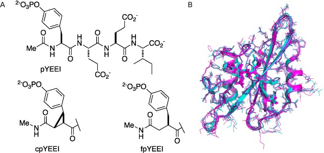
Molecules simulated in this study. (A) The three peptides, denoted as canonical (pYEEI), constrained (cpYEEI), and flexible (fpYEEI). (B) Overlay of the Src SH2–peptide complex X-ray structures used to build initial models: 2 chains from the SH2–cpYEEI complex (1IS0, cyan) and 3 chains from the SH2–pYEEI complex (1SPS, magenta). Bound peptides are rendered with thick lines, protein side-chains in thin lines and the protein main-chains in ribbons.

A set of 40 simulations was generated for each of the six systems. Five sets of starting coordinates for each system were obtained from the crystallographic coordinates of the Src SH2—cpYEEI complex (PDB code 1IS0(29)), containing two copies of the complex in the asymmetric unit, and Src SH2 with a bound 11-residue peptide including the canonical pYEEI sequence (PDB code 1SPS(30)), containing three copies of the complex in the asymmetric unit. An overlay of the crystallographic structures is shown in Figure 1B. Among these five sets of crystallographic coordinates, the pairwise rms differences between Src SH2 Cα coordinates range from 0.49 to 0.83 Å, and between all-heavy atoms from 0.97 to 1.54 Å. For the three complexes, the crystallographic ligand was alchemically mutated to the desired pseudopeptide to yield five sets of starting coordinates. Velocities were randomized using random seeds for each of the five starting coordinate sets to establish the 40 unique starting conditions.

SH2 complexes and peptides were prepared for simulations using CHARMM version c35,³¹ and production runs were performed with NAMD³² using the CHARMM27 all-atom force field³³ with CMAP dihedral angle correction.³⁴ Parameters for the nonstandard cpY and fpY residues were described previously.¹ Solutes were solvated with 6840 TIP3P water molecules for SH2–ligand complexes, or 2310 water molecules for the free peptides in octahedral boxes, so that the box edges were at least 14 Å from the solute. Nonbonded lists were generated with a 14 Å cutoff using the BYCUBES method,³¹ and nonbonded interactions were calculated with a 12 Å cutoff and truncation functions applied starting at 10 Å. van der Waals interactions were treated with an atom-based switching function and short-range electrostatics with an atom-based shifting function. Long-range electrostatic interactions were estimated using the particle mesh Ewald method. The energy of the initial systems was minimized for 500 steps with the steepest descent algorithm and then with the adopted basis Newton–Raphson algorithm for 1000 steps or until the energy change between steps was less than 1 kcal/mol, first with the solute atoms fixed, then with harmonic constraints on solute main chain atoms, then finally without constraints.

Molecular dynamics trajectories were calculated with the leapfrog integrator using a 1 fs time step. Constant pressure and temperature (CPT) Nosé–Hoover–Andersen–Klein dynamics used a reference pressure of 1 atm and temperature of 298 K. Simulations were equilibrated for 2500 ps. Production runs of 10 ns were recorded for each of the 40 simulations per system, yielding a total MD run time of 400 ns for each of the six systems. Coordinates were saved every 1 ps. Potential energy values for estimating binding enthalpy were calculated from postprocessing of the trajectories.

Relative Binding Enthalpy Calculation

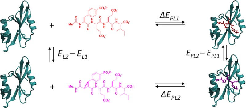
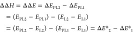
Relative enthalpies (ΔΔH) for binding various ligands to a single protein were calculated by the direct method of estimating the internal energy of end-states according to Scheme 1. For a protein (P), two ligands (L1 and L2), and protein–ligand complexes (PL1 and PL2), ΔΔH is estimated from internal energy given there is negligible change in molecular volume between the bound and unbound states at constant pressure. From the thermodynamic cycle in Scheme 1,

1

with the energy difference, ΔE*, for each ligand being

2

where ⟨···⟩ is the expectation, or time-averaged value obtained from simulations (details given below), and “*” emphasizes the quantity is not the true binding energy given that the energy of the unbound state of the protein (⟨E_P⟩) does not appear in eq 1. An unbound protein simulation is omitted in the analysis because ⟨E_P⟩ cancels in the relative binding enthalpies.

Scheme 1. Thermodynamic Cycle for the Relative Binding Enthalpy Calculation by the Direct End-State Method.

The internal energy of the system is from the molecular mechanics force field of simulations calculated for each protein–ligand complex and the unbound ligand. The total system energy, E^T, can be partitioned into components corresponding to the geometry and intramolecular nonbonded interactions of the solute, E^UU, where the solute is either PLn or Ln, the intermolecular interactions between the solute and solvent, E^UV, and interactions between water molecules, E^VV:

3

Mean Energy Values and Uncertainties

A set of trajectories for each state was obtained by calculating multiple, independent MD trajectories. Multiple simulations are considered to provide a broader sampling of conformational space than a single simulation extended for an equivalent total simulation time.³⁵⁻³⁸ The simulations in this study were calculated independently and not subjected to replica exchange³⁹ or other collective weighting scheme,⁴⁰ and thus the resulting trajectories serve as a set of repeated measurements of the energy with mean values distributed across the potential energy surface.

The local mean energy, , is estimated from the molecular mechanics force field of the simulations from a single trajectory as the time-average value for trajectory k over the time period corresponding to N snapshots,

4

where E_k,n is the energy value of the nth snapshot of the kth trajectory.

The expected energy value for the set of trajectories, ⟨E⟩, is determined from the set of local means, E̅_k, of the individual trajectories. For K trajectories, the ensemble mean is

5

For the total ensemble here, K equals 40 trajectories and N corresponds to the number of snapshots from a 10 ns trajectory. Certain of the results that follow examine convergence by using cumulative averages for which the value N is varied. Analysis of the simulation ensemble by the simple average defined with eq 5 assumes individual trajectories, k, to be equally likely, an assumption discussed in Results.

The uncertainty in the energy values estimated from K independent trajectories was obtained by the bootstrap method⁴¹ rather than estimating the error from variances of individual trajectories. For a small sample number, the uncertainty obtained by the bootstrap method is expected to better estimate the width of the underlying Gaussian distribution of mean values than does the standard error. Additionally, applying the bootstrap method to K independent trajectories satisfies the condition of independence among sample observations; thus, the uncertainty of the energy values is reliably estimated using the bootstrap method. 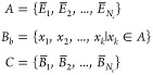Given the set A of K local means determined for the independent trajectories, a set C of synthetic ensemble means, , was constructed, where each is the mean of K values selected randomly from the set A. The uncertainty of the ensemble mean value, δ_⟨E⟩, is the standard deviation of the bootstrap sample C,

6

7

where N_c is the number of resampled ensembles in the bootstrap sample, and C̅ is the average of the bootstrap sample. In this study, N_C equals 400. The 95% confidence interval (CI) is calculated from the standard deviation of the bootstrap means: 1.96δ_⟨E⟩. We also calculated the 95% CI from standard error of the local mean values for comparison (see Supporting Information). As expected, the two procedures approach each other as the number of simulations increases so that the bootstrap error and the standard error are similar for our 40 trajectories.

To examine the efficiency for estimating the expected value of the energy, we estimated uncertainty of mean energies for a range of schedules by varying both the number of simulations and the time period of each simulation for a given total simulation time. Bootstrap analysis was applied to randomly selected subsets of trajectories from the ensemble to assess the convergence of the ensemble mean with increasing time per simulation (N) and number of simulations (K). We find the mean energy value for 2 ≤ K ≤ 40 individual trajectories from 50 to 10000 ps, or 50 ≤ N ≤ 10000 (eq 4). This set of K mean values, E̅_K^N, is used to generate a bootstrap sample of size 100, and the standard error from sample i, δ_⟨E⟩, calculated by eq 7. The random selection of K trajectories is repeated 50 times and the final standard error determined from the average variance

8

The matrix of 39 × 9951 standard error values is visualized in a two-dimensional plot.

Two-Dimensional Histograms of Total Energy and rmsd

The potential energy of each system was obtained from postprocessing the corresponding trajectories using the ENER module in CHARMM. For every system, the conformation having the lowest potential energy was chosen as the reference structure for subsequent rms deviation calculations. The rmsd of the backbone heavy atoms (N, Cα, C) with respect to the lowest-energy conformation at every snapshot was calculated using the CORREL module in CHARMM. Then, the ensemble of energy and rmsd values were binned into a two-dimensional histogram to illustrate the distribution of population sampled in the energy–rmsd phase space.

All-Against-All (Pairwise) rmsd Calculations

For every system, the backbone heavy atoms were aligned to the lowest-energy conformation before pairwise rmsd calculations. Nonweighted pairwise rmsd values were calculated among the 40 aligned trajectories using backbone heavy atoms every 10 ps. Subsequently, calculated pairwise rmsd values were binned into histograms and plotted.

Results and Discussion

Estimates of Relative Binding Enthalpies

The relative binding enthalpy for three Src SH2–ligand complexes was estimated by the direct method (eq 1) using ensemble-averaging and the a priori assumption that the trajectories sample the same energy basin and have equal likelihood (eq 5). Forty 10 ns trajectories, a total of 400 ns simulation time, were generated from equilibrium molecular dynamics simulations for each of the bound and unbound states of the three Src SH2 ligands illustrated in Figure 1. The two pseudopeptides, cpYEEI and fpYEEI, differ from pYEEI by altering only the pY residue to a constrained isopropyl form or its flexible analogue, respectively. Mean energy values, ⟨E^T⟩, and the 95% confidence intervals determined from the bootstrap analysis for each system are presented in Table 1, along with the calculated energy differences relative to the Src SH2–pYEEI complex, ΔΔE, and the corresponding experimental enthalpies, ΔΔH. The 95% confidence interval (CI) from the bootstrap analysis in the mean total energy is ±1.6 to ±2.6 kcal/mol for the complexes, and ±0.5 to ±0.8 kcal/mol for the free peptide simulations. Even though the mean energies for the simulation systems are on the order of 10⁵ kcal/mol, the magnitude of the ΔΔE values is small (0.14 and 2.2 kcal/mol) and of the same order as the experimental values (1.5 kcal/mol and −1.2 kcal/mol). Nonetheless, the 95% CI in ΔΔE is approximately 2 to 3 kcal/mol, which is similar magnitude to the experimental differences, so that rank order cannot be reliably predicted in this case of Src SH2 binding analogue peptides.

Table 1. Ensemble Mean Values and 95% Confidence Interval (CI) for the Total Potential Energy, E^T, and the Relative Binding Energies, ΔΔE, from Calculations, Along with the Relative Binding Enthalpies, ΔΔH, from Experiment.

	total system energya (kcal/mol)
	⟨ET⟩	95% CI
SH2–pYEEI	–73777.8	±2.1
SH2–cpYEEI	–73741.3	±1.6
SH2–fpYEEI	–73753.9	±2.6
pYEEI	–24137.1	±0.5
cpYEEI	–24100.8	±0.6
fpYEEI	–24115.5	±0.8

	relative binding enthalpyb (kcal/mol)
	calcd. ΔΔE	95% CI
pYEEI	0.0	±2.2
cpYEEI	0.1	±2.2
fpYEEI	2.2	±3.2

	exptl. ΔΔHc	δexp
pYEEI	0.0	0.07
cpYEEI	1.5	0.06
fpYEEI	–1.2	0.06

^aEnsemble mean energy from 40 10 ns trajectories according to eq 5 with uncertainty from bootstrapping according to eq 7.

^bΔΔE = (⟨E⟩_SH2–X – ⟨E⟩_X) – (⟨E⟩_SH2–pYEEI – ⟨E⟩_pYEEI)

^cExperimental ΔΔH values determined from ITC ΔH data^1,29 and propagated errors determined from experimental standard deviations.²⁹

To better understand the potential for estimating differences in the enthalpies of binding small peptides to a globular protein, in the following subsections we examine the convergence behavior of the mean energy values of the set of trajectories, including the relative binding energies for the SH2–ligand complexes calculated from the MD trajectories. An energy distribution of conformations sampled from multiple trajectories is used to characterize the alternative regions in conformational space visited by the trajectories.

Convergence and Certainty of Energy Values and Relative Binding Energy

The direct method for estimating the relative enthalpy of binding, ΔΔE = ΔE₂^* – ΔE₁, depends on the total potential energy of the system for the SH2–peptide complexes and free peptide ligands (Table 1). Thus, the ability to resolve the relatively small energy differences of ΔΔE from the large E^T values relies on determining the average values of the energies with high confidence. A necessary condition for this reliability is that the value be well converged, although it is recognized that such convergence does not guarantee sampling is complete in a true global sense and can be an indicator of only a localized sampling.⁴² The ensemble-averaged value as a function of the production time per simulation used for averaging is one indicator for the convergence of the estimated value. This cumulative ensemble average for ΔΔE, as well as for E^T of the complexes and peptides and ΔE*, is shown in Figure 2. The limiting slopes (Table 2) for E^T are approximately −0.2 to −0.6 kcal/mol·ns for the complexes and 0.02 to 0.08 kcal/mol·ns for unbound peptides. These cumulative averages of the energy from the ensemble mean over 40 trajectories are considerably more stable than the cumulative average of a single trajectory; single-trajectory cumulative averages fluctuate over much larger magnitudes and have limiting slopes that range from 2.1 to −2.3 kcal/mol (see Supporting Information). The absolute difference in the ensemble-mean energy, ΔE*, Figure 2C continues to drift at the end of the 10 ns simulation time period as a result of the difference in the limiting slopes for the complex and peptide ensemble averages. The drift in ΔE* partially cancels when comparing two complexes so that the relative energies, ΔΔE, plotted in Figure 2D with pYEEI as the reference ligand 1, appear better converged with flatter curves at shorter times. Nevertheless, smaller limiting slopes in E^T over a longer simulation time period would yield greater confidence in the calculated values for ΔΔE and estimating differences of one to two kcal/mol. The limiting slopes in Figure 2A suggest that 400 ns molecular dynamics simulations are not sufficient to exhaustively sample the complex superbasin of the potential energy surface of these reasonably “simple” protein complexes.

Figure 2.

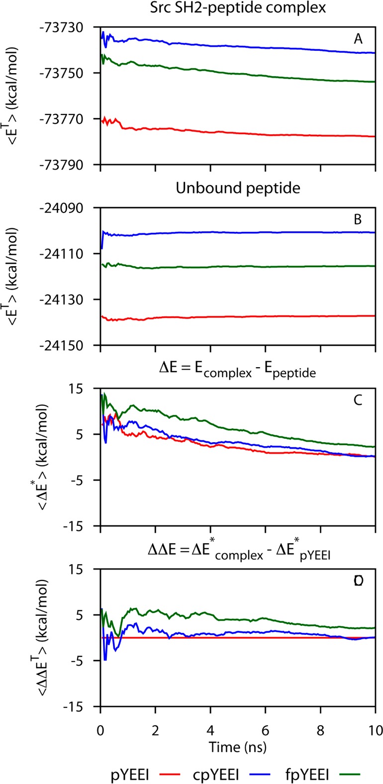
Convergence of the 40-trajectory ensemble averages (eq 5) accumulated over increasing production time of the simulations for various energies: (A) the total energy (E^T) for the complexes, (B) total energy for the ligands, (C) effective binding enthalpies (ΔE*), and (D) relative binding enthalpies (ΔΔE). Red, SH2–pYEEI or pYEEI; blue, SH2–cpYEEI or cpYEEI; green, SH2–fpYEEI or fpYEEI. Points in C are shifted by subtracting the final value of ΔE* for pYEEI (10 ns/simulation).

Table 2. Least-Squares Fitted Slopes at the Long-Time Limit of the Ensemble Mean Cumulative Averages, the 8 to 10 ns Regions in Figure 2.

		slope (kcal/mol·ns)
⟨ET⟩	SH2–pYEEI	–0.16
	SH2–cpYEEI	–0.56
	SH2–fpYEEI	–0.36
⟨ET⟩	pYEEI	0.08
	cpYEEI	0.02
	fpYEEI	0.06
⟨ΔET⟩	pYEEI	–0.26
	cpYEEI	–0.56
	fpYEEI	0.44
⟨ΔΔET⟩	pYEEI	0.000
	cpYEEI	−0.32
	fpYEEI	–0.16

The dependence of the statistical certainty of the energy estimates on simulation time was determined using the bootstrap method⁴¹ (see Methods). The decrease of the 95% CI for ⟨E^T⟩ is shown in Figure 3 for the Src SH2–pYEEI with a 2-dimensional plot as a function of the length of the individual trajectories and as a function of the number of trajectories, for which a subset of the 40 trajectories is used in the bootstrap analysis. Black contour lines in the figure denote a constant computer simulation time according to the combined number and length of the individual trajectories. Analogous plots are provided in Supporting Information for the other systems. The uncertainty converges approximately as expected from sampling a single statistical population; the 95% CI for 100 ns computer time is ranges from 3 to 4 kcal/mol and for 400 ns computer time is 2.2 kcal/mol. The efficiency for diminishing the statistical uncertainty is nearly uniform along the contour lines for computer times greater than 200 ns, so that increasing the time period of the simulation or the number of simulations is equally effective.

Figure 3.

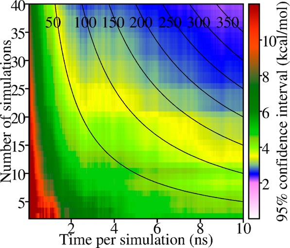
Convergence of the statistical uncertainty in the estimate of potential energy of SH2–pYEEI. The 95% CI (1.96 δ_⟨E⟩) for E^T narrows with increasing number of simulations and time per simulation. Uncertainties were determined by bootstrap for subsets of the 40, 10 ns SH2–pYEEI simulations as detailed in Methods. Solid black curves mark subsets with equal total simulation time (labeled in ns) spread over the number of simulations and the time per simulation.

In addition to the convergence of E^T, the convergence of the estimate for the components of the total potential energy was evaluated. The cumulative ensemble-averaged values for the difference in binding enthalpy contributed by solute–solute (E^UU), solute–solvent (E^UV), and solvent–solvent (E^VV) interactions are shown in Figure 4. (Note the large scale of A relative to the panels B–D). Because the total energy is constant but partitioned among these three components, the convergence is slower depending on the relaxation time for partitioning. The convergence behavior manifests in the time dependence of the cumulative average of the ensemble component energies is therefore poor and the estimates vary tens of kcals/mol over the full 400 ns simulation time.

Figure 4.

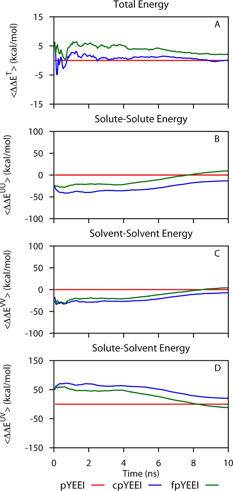
Convergence of cumulative averages as in Figure 2 for the decomposition of relative binding energies into solute and solvent contributions for the three SH2 complexes. (A) Total potential energy shown for comparison (note the difference in scale of the ordinate between the total potential energy and the component terms.); (B) solute–solute energy; (C) solvent–solvent energy; (D) solute–solvent energy. All difference terms are calculated relative to values for Src SH2–pYEEI.

Overlap of Trajectories in Conformational Space

The cumulative ⟨E^T⟩ values of individual trajectories vary, as noted above and shown in Supporting Information. This behavior raises the question of whether the trajectories sample the same energy basin in the conformational space of the bound complex, as assumed a prior for ensemble averaging. To gain insight into the actual overlap and nature of the conformational regions populated by individual trajectories, we examine distributions in an energy–rmsd system, a natural choice to address this question. The energy is the total potential energy and the rmsd value is the pairwise root-mean-square difference in the N, Cα, C atoms of the SH2 backbone between the trajectory snapshots and the structure with the lowest potential energy in the 40-trajectory ensemble.

Presented in Figure 5 are the projected distributions in the energy–rmsd space for the three Src SH2–peptide complexes. Results for one complex are shown in a group of two rows: SH2–pYEEI is the top group, SH2–cpYEEI is the middle group, and SH2–fpYEEI is the bottom group. Each plot in the top row displays the projection for simulations initiated from five different sets of coordinates, while the plots in the bottom row correspond to the same individual simulations but separated by those initiated from one set of coordinate with five different velocities. (Twenty-five of the forty trajectories are shown to facilitate comparison of the initial conditions that vary by either coordinates or velocities.) Thus, a distribution in the top rows indicates the coverage of conformational space achieved by starting simulations with different initial coordinates, while that in the bottom rows reflects the coverage achieved by starting simulations with one initial coordinate set and varying velocities, as is more typically done to generate multiple trajectories. The fluctuations in energy values cover a broad range of roughly 500 kcal/mol for values of rmsd that mostly vary in the region from 1.0 to 1.5 Å. Some distributions in panel A through J show one peak with a maximum that is more or less centrally positioned, while others show two peaks distinguished along the rmsd coordinate. One might anticipate that multiple trajectories initiated with different initial coordinates (top rows A–E) might show greater dispersion in the energy–rmsd distribution than multiple trajectories initiated with the same coordinates but varying velocities (bottom panels F–J); however, that is not the case: the dispersions in the distributions do not differ significantly.

Figure 5.

Two-dimensional projection for the distribution of E^T as a function of Src SH2 rmsd for (top) SH2–pYEEI, (middle) SH2–cpYEEI, and (bottom) SH2–fpYEEI. The rmsd is summed over N, Cα, C backbone coordinates of a snapshot against the lowest-energy structure of the 40-trajectory ensemble. Top rows (A–E): each plot represents five trajectories started with different initial coordinates. Bottom rows (F–J): each plot represents five trajectories started with the same initial coordinates from the PDB code and chain identifier for protein and peptide indicated in the plot. Panel K: 40 trajectories.

Nearly all of the individual trajectories visit two or more regions in energy–rmsd space (see Supporting Information), consistent with different trajectories sampling overlapped parts of conformational space and that the barriers in the underlying potential energy surface giving rise to differences between the trajectories are low. In addition, the combined population from the 40-trajectory ensemble (panel K) is one broad peak in energy–rmsd space with a single maximum indicating the overlap of individual trajectories. Together, the energy–rmsd distributions are consistent with the individual trajectories sampling one superbasin in conformational space, albeit sampling different parts of that basin, and thus support this assumption for ensemble averaging.

The different regions apparent in plots A–J are close in energy for a given Src SH2–peptide complex. For each of the three complexes, regions in energy–rmsd were determined from the distinct peaks in panels A–J, and the mean energy calculated from the conformations in the 400 ns ensemble falling into a given region. The average energies and populations for each energy–rmsd region are listed in Table 3. The mean energies differ by a few kcal/mol; the largest difference is approximately 7 kcal/mol. Thus, the peak regions in Figure 5 are nearly degenerate in energy.

Table 3. Average Energy of Snapshots Falling in the Different Peak Regions Populated in the Energy–rmsd Space of the Src SH2 Complexes.

complexes	rmsda range (A)	E̅T (kcal/mol)	σETb (kcal/mol)	populationc
SH2–pYEEI	0.42 to 1.25	–73779.0	132.0	231 461
	1.25 to 1.96	–73776.2	132.4	168 539
SH2–cpYEEI	0.46 to 1.08	–73742.0	131.9	93 600
	1.08 to 1.58	–73741.2	132.4	281 492
	1.58 to 2.32	–73740.2	132.4	24 908
SH2–fpYEEI	0.45 to 1.08	–73756.6	132.8	170 977
	1.08 to 1.38	–73752.7	132.5	164 773
	1.38 to 1.83	–73750.0	132.5	52 797
	1.83 to 2.50	–73749.2	133.1	11 453

^aThe rmsd range is estimated for the peak regions.

^bσ is the energy standard deviation.

^cNumber of snapshots in the peak region.

Conclusion

The relative enthalpies for the binding of the 106-residue Src SH2 domain to three flexible peptides were estimated using the direct method of MD determined from the end-states. Notably, the estimated ΔΔE values were of similar magnitude as the differences in the experimental enthalpies, which are only 1–3 kcal/mol. Nonetheless, the rank order was not predicted correctly for these three complexes. The statistical error in the estimates for ΔΔE from 40 10 ns simulations for each bound and unbound peptide system is 2 to 3 kcal/mol (Table 1). Based on cumulative ensemble-averaged values (Figure 2), the end-state energies are not fully converged; the cumulative averages for E^T of the complexes have a limiting rate of change from 0.2 to 0.6 kcal/mol·ns, although there is some cancellation in the ΔΔE values so that these appear better converged. These results support the application of the direct method of MD simulations to predict relative binding enthalpies for ΔΔH values greater than 3 kcal/mol. Longer simulations are expected to yield improvements over the predictions reported here, which correspond to 400 ns total simulation time. Likely, the most successful application of the direct method of MD simulations for predicting ΔΔH values will be to complexes that are conformationally well-ordered and absent of longer-time scale conformational fluctuations that substantially alter the protein energetics.

Multiple trajectories starting from closely related but alternative configurations, or different velocities exhibit different E̅_K^T values with poorer convergence than the ensemble-averaged values. That individual trajectories have different energies suggests that trajectories need to be weighted.³⁵ How to weight trajectories is an important but difficult consideration. The analysis here has utilized a simplistic, unweighted ensemble averaging with the a priori assumption that all trajectories are equally likely. Clustering in energy–rmsd space indicates the trajectories sample the same basin and the apparent difference in mean energy value between trajectories is due to sampling alternative local regions of this superbasin. Clearly, the sampling is incomplete. For more reliable estimates of binding enthalpies, additional theoretical development is needed; in particular, the direct method would gain from reliable methods to achieve canonically distributed starting conditions both in terms of reaching statistical certainty efficiently and, importantly, complete sampling for accurate ensemble-averaged end-state energy values.

An advantage of the direct method for estimating the relative binding enthalpies is its basis on the total energy of the system rather than a summation of various energy terms, for example solvation energy plus protein internal energy. The fluctuations in the total energy are small relative to the fluctuations of any set of component energy terms; component terms freely exchange energy and thus exhibit large fluctuations. Therefore, the certainty in the total energy converges more rapidly while component energies by nature are more difficult to converge. Nonetheless, decomposition of thermodynamic values can provide useful insight where accurate quantification is not essential. An example we note here is the observation that the fluctuations in the cumulative mean values for the components ΔΔE^UU, ΔΔE^VV, and ΔΔE^UV have the same convergence behavior and are close to being perfectly correlated either negatively (ΔΔE^UV with either ΔΔE^UU or ΔΔE^VV) or positively (ΔΔE^UU with ΔΔE^VV) (Figure 4). Correspondingly, an inverse correlation of E̅_k^UU and E̅_k is observed upon examination of the mean values from individual trajectories (Supporting Information). The E̅_k^UV variance among the multiple trajectories is large compared to E̅_k and approximately equal to the sum of the variances in E̅_k^UU and E̅_k. This macroscopic behavior is reminiscent of the microscopic property whereby the reaction field solvation energy cancels the Coulombic interaction.

Supporting Information Available

Plots of the cumulative average of E^T for the individual trajectories of the six simulations systems (Figure S1); plots analogous to Figure 4 showing 95% CI results for the ensemble-averaged E^T values for SH2–cpYEEI, SH2–fpYEEI (Figure S2), and the three unbound peptide ligands (Figure S3), as well as the ensemble-averaged E^UU, E^VV, E^UV, values for the three complexes (Figure S4) and unbound peptide ligands (Figure S5); plots of pairwise, or all-against-all, rmsd distributions to examine overlap of individual trajectories in sampling conformational space (Figure S6); a plot showing the deviation from the ensemble mean energy of the local mean energy from individual trajectories, where the energy is the total potential, E̅_k^T, or the highly correlated component terms E̅_k, E̅_k^VV, and E̅_k (Figure S7); a plot showing 95% CI from standard error calculation for ET values (Figure S8) and for E^UU, E^UV, E^VV values (Figure S9) for complex SH2-pYEEI. Table S1 lists the limiting slopes in the cumulative potential energy of forty trajectories for each of the three SH2-peptide simulations. This material is available free of charge via the Internet at http://pubs.acs.org.

Author Present Address

^‡ Department of Chemistry, University of Oulu, PO Box 3000, FIN-90014 Oulu, Finland

Author Contributions

^† A.R., D.P.H., and J.M.W. contributed equally to this work.

The authors declare no competing financial interest.

Funding Statement

National Institutes of Health, United States

References

- Ward J. M.; Gorenstein N. M.; Tian J.; Martin S. F.; Post C. B. Constraining Binding Hot Spots: NMR and Molecular Dynamics Simulations Provide a Structural Explanation for Enthalpy–Entropy Compensation in SH2–Ligand Binding. J. Am. Chem. Soc. 2010, 1323211058–11070. [DOI] [PMC free article] [PubMed] [Google Scholar]
- Yu B.; Martins I. R. S.; Li P.; Amarasinghe G. K.; Umetani J.; Fernandez-Zapico M. E.; Billadeau D. D.; Machius M.; Tomchick D. R.; Rosen M. K. Structural and Energetic Mechanisms of Cooperative Autoinhibition and Activation of Vav1. Cell 2010, 1402246–256. [DOI] [PMC free article] [PubMed] [Google Scholar]
- Freire E. A Thermodynamic Approach to the Affinity Optimization of Drug Candidates. Chem. Biol. Drug Des. 2009, 745468–472. [DOI] [PMC free article] [PubMed] [Google Scholar]
- Chaires J. B. Calorimetry and Thermodynamics in Drug Design. Annu. Rev. Biophys. 2008, 371135–151. [DOI] [PubMed] [Google Scholar]
- Makhatadze G. I.; Privalov P. L. Energetics of Protein Structure. Adv. Protein Chem. 1995, 47, 307–425. [DOI] [PubMed] [Google Scholar]
- Chodera J. D.; Mobley D. L. Entropy–Enthalpy Compensation: Role and Ramifications in Biomolecular Ligand Recognition and Design. Annu. Rev. Biophys. 2013, 421121–142. [DOI] [PMC free article] [PubMed] [Google Scholar]
- Reynolds C. H.; Holloway M. K. Thermodynamics of Ligand Binding and Efficiency. ACS Med. Chem. Lett. 2011, 26433–437. [DOI] [PMC free article] [PubMed] [Google Scholar]
- Fenley A. T.; Muddana H. S.; Gilson M. K. Entropy–Enthalpy Transduction Caused by Conformational Shifts Can Obscure the Forces Driving Protein–Ligand Binding. Proc. Natl. Acad. Sci. U.S.A. 2012, 1094920006–20011. [DOI] [PMC free article] [PubMed] [Google Scholar]
- Gallicchio E.; Kubo M. M.; Levy R. M. Entropy–Enthalpy Compensation in Solvation and Ligand Binding Revisited. J. Am. Chem. Soc. 1998, 120184526–4527. [Google Scholar]
- Ford D. M. Enthalpy–Entropy Compensation is Not a General Feature of Weak Association. J. Am. Chem. Soc. 2005, 1274616167–16170. [DOI] [PubMed] [Google Scholar]
- DeLorbe J. E.; Clements J. H.; Teresk M. G.; Benfield A. P.; Plake H. R.; Millspaugh L. E.; Martin S. F. Thermodynamic and Structural Effects of Conformational Constraints in Protein–Ligand Interactions. Entropic Paradoxy Associated with Ligand Preorganization. J. Am. Chem. Soc. 2009, 1314616758–16770. [DOI] [PubMed] [Google Scholar]
- Simonson T.; Archontis G.; Karplus M. Free Energy Simulations Come of Age: Protein–Ligand Recognition. Acc. Chem. Res. 2002, 356430–437. [DOI] [PubMed] [Google Scholar]
- Gohlke H.; Klebe G. Approaches to the Description and Prediction of the Binding Affinity of Small-Molecule Ligands to Macromolecular Receptors. Angew. Chem., Int. Ed. 2002, 41152644–2676. [DOI] [PubMed] [Google Scholar]
- Lazaridis T.; Karplus M. Thermodynamics of Protein Folding: A Microscopic View. Biophys. Chem. 2003, 1001–3367–395. [DOI] [PubMed] [Google Scholar]
- Gilson M. K.; Zhou H. X. Calculation of Protein–ligand Binding Affinities. Annu. Rev. Biophys. Biomol. Struct. 2007, 36, 21–42. [DOI] [PubMed] [Google Scholar]
- Christ C. D.; Mark A. E.; van Gunsteren W. F. Basic Ingredients of Free Energy Calculations: A Review. J. Comput. Chem. 2010, 3181569–1582. [DOI] [PubMed] [Google Scholar]
- Deng Y.; Roux B. Computations of Standard Binding Free Energies with Molecular Dynamics Simulations. J. Phys. Chem. B 2009, 11382234–2246. [DOI] [PMC free article] [PubMed] [Google Scholar]
- Gallicchio E.; Levy R. M. Advances in All Atom Sampling Methods for Modeling Protein–Ligand Binding Affinities. Curr. Opin. Struct. Biol. 2011, 212161–166. [DOI] [PMC free article] [PubMed] [Google Scholar]
- Wereszczynski J.; McCammon J. A. Statistical Mechanics and Molecular Dynamics in Evaluating Thermodynamic Properties of Biomolecular Recognition. Q. Rev. Biophys. 2012, 45011–25. [DOI] [PMC free article] [PubMed] [Google Scholar]
- Karplus M. Dynamical Aspects of Molecular Recognition. J. Mol. Recog. 2010, 232102–104. [DOI] [PubMed] [Google Scholar]
- Genheden S.; Ryde U. Will Molecular Dynamics Simulations of Proteins Ever Reach Equilibrium?. Phys. Chem. Chem. Phys. 2012, 14248662–8677. [DOI] [PubMed] [Google Scholar]
- Levy R. M.; Gallicchio E. Computer Simulations with Explicit Solvent: Recent Progress in the Thermodynamic Decomposition of Free Energies and in Modeling Electrostatic Effects. Annu. Rev. Phys. Chem. 1998, 49, 531–567. [DOI] [PubMed] [Google Scholar]
- Lu N.; Kofke D. A.; Woolf T. B. Staging Is More Important than Perturbation Method for Computation of Enthalpy and Entropy Changes in Complex Systems. J. Phys. Chem. B 2003, 107235598–5611. [Google Scholar]
- Setny P.; Baron R.; McCammon J. A. How Can Hydrophobic Association Be Enthalpy Driven?. J. Chem. Theory Comput. 2010, 692866–2871. [DOI] [PMC free article] [PubMed] [Google Scholar]
- Shi Y.; Zhu C. Z.; Martin S. F.; Ren P. Probing the Effect of Conformational Constraint on Phosphorylated Ligand Binding to an SH2 Domain Using Polarizable Force Field Simulations. J. Phys. Chem. B 2012, 11651716–1727. [DOI] [PMC free article] [PubMed] [Google Scholar]
- Wan S.; Stote R. H.; Karplus M. Calculation of the Aqueous Solvation Energy and Entropy, as Well as Free Energy, Of Simple Polar Solutes. J. Chem. Phys. 2004, 121199539–9548. [DOI] [PubMed] [Google Scholar]
- Kubo M. M.; Gallicchio E.; Levy R. M. Thermodynamic Decomposition of Hydration Free Energies by Computer Simulation: Application to Amines, Oxides, and Sulfides. J. Phys. Chem. B 1997, 1014910527–10534. [Google Scholar]
- Davidson J. P.; Martin S. F. Use of 1,2,3-Trisubstituted Cyclopropanes As Conformationally Constrained Peptide Mimics in SH2 Antagonists. Tetrahedron Lett. 2000, 41499459–9464. [Google Scholar]
- Davidson J. P.; Lubman O.; Rose T.; Waksman G.; Martin S. F. Calorimetric and Structural Studies of 1,2,3-Trisubstituted Cyclopropanes As Conformationally Constrained Peptide Inhibitors of Src SH2 Domain Binding. J. Am. Chem. Soc. 2002, 1242205–215. [DOI] [PubMed] [Google Scholar]
- Waksman G.; Shoelson S. E.; Pant N.; Cowburn D.; Kuriyan J. Binding of a High Affinity Phosphotyrosyl Peptide to the Src SH2 Domain: Crystal Structures of the Complexed and Peptide-Free Forms. Cell 1993, 725779–790. [DOI] [PubMed] [Google Scholar]
- Brooks B. R.; Brooks C. L. 3rd; Mackerell A. D. Jr.; Nilsson L.; Petrella R. J.; Roux B.; Won Y.; Archontis G.; Bartels C.; Boresch S.; Caflisch A.; Caves L.; Cui Q.; Dinner A. R.; Feig M.; Fischer S.; Gao J.; Hodoscek M.; Im W.; Kuczera K.; Lazaridis T.; Ma J.; Ovchinnikov V.; Paci E.; Pastor R. W.; Post C. B.; Pu J. Z.; Schaefer M.; Tidor B.; Venable R. M.; Woodcock H. L.; Wu X.; Yang W.; York D. M.; Karplus M. CHARMM: The Biomolecular Simulation Program. J. Comput. Chem. 2009, 30101545–1614. [DOI] [PMC free article] [PubMed] [Google Scholar]
- Phillips J. C.; Braun R.; Wang W.; Gumbart J.; Tajkhorshid E.; Villa E.; Chipot C.; Skeel R. D.; Kalé L.; Schulten K. Scalable Molecular Dynamics with NAMD. J. Comput. Chem. 2005, 26161781–1802. [DOI] [PMC free article] [PubMed] [Google Scholar]
- MacKerell A. D. J.; Bashford D.; Bellott M.; Dunbrack R. L.; Evanseck J. D.; Field M. J.; Fischer S.; Gao J.; Guo H.; Ha S.; McCarthy J. D.; Kuchnir L.; Kuczera K.; Lau F. T. K.; Mattos C.; Michnick S.; Ngo T.; Nguyen D. T.; Prodhom B.; Reiher W. E.; Roux B.; Schlenkrich M.; Smith J. C.; Stote R.; Straub J.; Karplus M. All-Atom Empirical Potential for Molecular Modeling and Dynamics Studies of Proteins. J. Phys. Chem. B 1998, 102, 3586–3616. [DOI] [PubMed] [Google Scholar]
- MacKerell A. D.; Feig M.; Brooks C. L. Improved Treatment of the Protein Backbone in Empirical Force Fields. J. Am. Chem. Soc. 2004, 1263698–699. [DOI] [PubMed] [Google Scholar]
- Caves L. S. D.; Evanseck J. D.; Karplus M. Locally Accessible Conformations of Proteins: Multiple Molecular Dynamics Simulations of Crambin. Protein Sci. 1998, 73649–666. [DOI] [PMC free article] [PubMed] [Google Scholar]
- Monticelli L.; Sorin E. J.; Tieleman D. P.; Pande V. S.; Colombo G. Molecular Simulation of Multistate Peptide Dynamics: A Comparison between Microsecond Timescale Sampling and Multiple Shorter Trajectories. J. Comput. Chem. 2008, 29111740–1752. [DOI] [PubMed] [Google Scholar]
- Genheden S.; Ryde U. How to Obtain Statistically Converged MM/GBSA Results. J. Comput. Chem. 2010, 314837–846. [DOI] [PubMed] [Google Scholar]
- Grossfield A.; Zuckerman D. M.. Quantifying Uncertainty and Sampling Quality in Biomolecular Simulations. In Ann. Rep. Comput. Chem., Ralph A. W., Ed.; Elsevier: New York, 2009; Vol. 5, Ch. 2, pp 23–48. [DOI] [PMC free article] [PubMed] [Google Scholar]
- Sugita Y.; Okamoto Y. Replica-Exchange Molecular Dynamics Method for Protein Folding. Chem. Phys. Lett. 1999, 3141–2141–151. [Google Scholar]
- Christen M.; van Gunsteren W. F. On Searching in, Sampling of, and Dynamically Moving through Conformational Space of Biomolecular Systems: A Review. J. Comput. Chem. 2008, 292157–166. [DOI] [PubMed] [Google Scholar]
- Efron B.; Tibshirani R. Bootstrap Methods for Standard Errors, Confidence Intervals, and Other Measures of Statistical Accuracy. Stat. Sci. 1986, 1154–75. [Google Scholar]
- Straub J. E.; Rashkin A. B.; Thirumalai D. Dynamics in Rugged Energy Landscapes with Applications to the S-Peptide and Ribonuclease A. J. Am. Chem. Soc. 1994, 11652049–2063. [Google Scholar]
Associated Data
This section collects any data citations, data availability statements, or supplementary materials included in this article.