Abstract
Algorithms for fully automatic segmentation of images are often not sufficiently generic with suitable accuracy, and fully manual segmentation is not practical in many settings. There is a need for semi-automatic algorithms which are capable of interacting with the user and taking into account the collected feedback. Typically such methods have simply incorporated user feedback directly. Here we employ active learning of optimal queries to guide user interaction. Our work in this paper is based on constrained spectral clustering that iteratively incorporates user feedback by propagating it through the calculated affinities [17]. The original framework does not scale well to large data sets, and hence is not straightforward to apply to interactive image segmentation. In order to address this issue, we adopt advanced numerical methods for eigen-decomposition implemented over a subsampling scheme. Our key innovation, however, is an active learning strategy that chooses pairwise queries to present to the user in order to increase the rate of learning from the feedback. Performance evaluation is carried out on the Berkeley segmentation and Graz-02 image data sets, confirming that convergence to high accuracy levels is realizable in relatively few iterations.
Index Terms: Interactive image segmentation, affinity propagation, pairwise querying, active learning, spectral clustering
I. Introduction
Image segmentation refers to the task of grouping image pixels into a meaningful partition such that pixels falling in the same group are similar to each other, and different than those in other groups, in terms of a perceptually meaningful similarity measure. Segmentation often is used as a pre-processing step before higher level image processing or understanding. Manually segmenting images can be laborious and time-consuming, especially for large images, and can be prone to subjectivity. At the same time, developing a generic unsupervised segmentation algorithm that can be accurately applied to all, or even many, types of images is not straight-forward. This is mainly because automatic image segmentation is known to be an ill-posed problem [3] in the sense that images can be segmented differently depending on hard-to-specify high level goals. For example, in a street image, the user might desire to segment cars or buildings depending on the underlying application: urban traffic or architecture respectively. Alternatively, supervised algorithms are provided with training sets to learn what the user wants to segment. This strategy, although not as tedious as manual segmentation, still requires the user to do the laborious task of fully labeling a sufficient number of training images to assure generalization over the full class of images of interest.
Hence one promising approach, which has recently received more attention, is to leverage both automatic and manual segmentation in a user-interactive fashion that is tunable to the user’s target segmentation outcome with as few interactions as possible. In typical examples of these methods, a semi-automatic segmentation algorithm is constructed over a classical fully-automatic core method, where the user’s feedback is viewed as a set of constraints on the core.
The user constraints can be either on class assignment of individual pixels or pairwise relationships between them. The former suggests requesting labels for a subset of individual pixels (individual constraints) [3], [7], [9], [11]–[13], [16], [23], [27] and is usually used with supervised cores, while the latter is based on specifying whether a pair of pixels should be in the same or different clusters (pairwise constraints) [17], [33], [35] and is more compatible with unsupervised methods1. There are also methods encoding both types of constraints in their formulation [4]. Here, since we approach the segmentation problem from an unsupervised point of view, we work with pairwise labeling.
Semi-automatic algorithms inherit some basic features from their core methods. One principal distinction among segmentation methods is whether they use features extracted from boundaries or regions. A boundary-based core method uses the constraints over the boundary locations [5], [21] to relocate them while a region-based core exploits constraints on the region assignments [2], [7], [8], [24] to re-characterize and re-group the pixels. Boundary-based interactive techniques are easy to run with the user in a loop [14]; however, the information provided by boundary constraints is local and not easy to propagate. Methods introduced by Zhang and Ji [34] and Lu and Carreira-Perpiñán [17] are two examples of region-based methods that interact with the user iteratively. In the former [34] a probabilistic framework was built for semi-supervised segmentation, whereas the latter [17] presented a constrained spectral clustering method. The major bottleneck of Lu and Carreira-Perpiñán’s work is the expensive computational cost, which makes its application to large images impractical. This difficulty is mainly due to the eigen-decomposition required by its spectral core method (O(ñ3) with ñ as the number of samples).
There have been two main directions reported to scale up spectral clustering: (1) using numerical eigen-decomposition methods, as in the pioneering work of Shi and Malik [30] where the Lanczos method (with complexity of O(ñ3/2)) was employed to estimate the first few eigenvectors; and (2) data subsampling; for instance Fowlkes et. al [6] exploited the Nystrom sampling technique (with complexity O(ñn + n3) where n is the number of samples) for estimating eigenvectors of the affinity matrix. In this work, we used both types of strategies for further acceleration: subsampling the pixels using the so-called novelty selection method [26], which tries to avoid choosing redundant samples in a greedy fashion, and estimating the eigenvectors with a numerical method called orthogonal iteration [10], a generalization of the power method to multiple eigenvector estimation.
Speed issues also arise in terms of convergence rate when the interactions are done iteratively: it is desirable for the algorithm to choose constraints such that the number of interactions required to achieve the desired segmentation is reasonably small. This is a learning problem; as an educational metaphor consider a learning system, with a student (here the algorithm asking for individual/pairwise constraints) and a teacher (corresponding to the source of labels, or oracle) to help the student with answers. A sophisticated method of teaching is to involve the student in the learning process by guiding him/her to ask about the most troublesome topics. The problem of how to choose questions to learn as fast as possible is widely studied under the title of active learning (see [29] for a tutorial).
Computing the uncertainty about the segment assignment of individual pixels in a given segmentation is common in active semi-automatic segmentation techniques: as two examples, Zhang and Ji [34] ranked image entities based on their impact on the uncertainty of a constructed Bayesian Network model; and Top et. al [31] selected the slice with the most uncertainty to be labeled for segmenting 3D images interactively. Almost all reported segmentation methods equipped with active learning, request user labels for individual pixels. Here, since we focus on pairwise constraints, we ask about the comparative assignments of pairs of samples.
The interactive framework described here builds on a constrained spectral clustering core method using affinity propagation [17], where user feedback is used to learn new pairwise similarities. The central idea relies on the assumption of a Gaussian process prior over the vector containing the segmentation assignments. Here we use this algorithm iteratively, alternating between updating the segmentation and requesting pairwise constraints from the user, until the user is satisfied with the result (or in effect, the iterations converge). We scale up the original algorithm from the synthetic small data sets in [17] to handle large images by reducing the computational burden of each iteration. Additionally, we accelerate the learning process by actively learning which pairs of pixels to query. Focusing on binary segmentation problems, the performance of our algorithm is evaluated using the Berkeley segmentation dataset [20]. We show that it converges reasonably quickly to the target segments even though the input image is represented only by naive pixel-wise features. Similar to other stochastic algorithms observing partial labels coming from the user at each iteration does not guarantee monotonically improving performance; however when it is likely to see performance fluctuations along the iterations, the algorithm is expected to climb up to a reasonable result at the convergence. We analyzed stability through the softness parameter of affinity propagation and found that a well-chosen dynamic schedule performed best in terms of convergence rate. We also investigated how generalizable this schedule is by running it over two other sets of images chosen from Graz-02 data set [19], [25].
II. Preliminaries
In this section, after introducing our notations, we give an overview of the graph-cut problem for which spectral clustering gives an approximate solution, and then briefly describe the constrained spectral clustering algorithm based on affinity propagation which we adopt.
A. Notations
Throughout this paper, lower case letters such as a ∈ ℝ denote scalar variables; lower case bold-faced letters like a ∈ ℝn, n > 1 denote vectors; upper case letters like A represent sets and upper case bold-faced letters like A ∈ ℝn×m, n, m > 1 represent matrices. Moreover, aij denotes (i, j)’th element of matrix A and ak indicates its k’th column. In ∈ ℝn×n and 0n×m ∈ ℝn×m denote the identity and all-zeros matrices respectively, and 1n represents an n × 1 all-ones vector. We represent the i’th canonical vector by ei. The operator |.| returns the absolute value for scalars and cardinality for sets. The indicator function
 (a) indicates if the object a belongs to set A:
Finally, p denotes a probability density function (pdf) while P denotes a probability mass function (pmf).
B. Spectral Clustering
Let us represent each image as a set of feature vectors X = {x1, …, xn} ∈
 ⊆ ℝd where xi collects the features of the i’th pixel. In order to construct a graph over the image, we use a positive definite kernel k(·, ·) :
 ×
×
 → ℝ+ for measuring similarity between pairs of data points. The Gaussian kernel is a common function of this type:
| (1) |
where Σ ⪰ 0 is the covariance matrix. Here the kernel is assumed to have uncorrelated variables yielding a diagonal matrix Σ with possibly different diagonal terms. We collect the calculated similarities leading to a positive definite affinity matrix2 K ≻ 0 such that kij = k(xi, xj). This matrix induces an undirected graph G = (X, K) over the set of pixels X and with edge weights defined by equation (1).
The binary graph-cut problem is how to bipartition X into two balanced groups C = {C1, C2}, such that the sum of the similarities between nodes in different groups is minimized. One way of solving this NP-complete problem is by relaxing the discreteness and defining a continuous cluster assignment vector f that can be estimated by eigen-decomposition of the Laplacian matrix3 where D is the degree matrix whose i-th diagonal term is dii = Σj kij. In order to discretize this solution, k-means clustering is usually used over the rows of the partially estimated eigenvector matrix [22].
C. Affinity Propagation
In the method proposed by Lu and Carreira-Perpiñán [17], constraints are propagated through pairwise affinities by assuming that f is a realization of a Gaussian process:
| (2) |
where the covariance, K, is the similarity matrix of the data. A pairwise constraint ωij between two given pixels xi and xj, is either a must-link (ωij ∈
 ) or a cannot-link (ωij ∈
 ), ensuring that the points are in the same or different clusters respectively. In the affinity propagation technique [17], ωij is modeled probabilistically such that fi and fj tend to have the same or different signs if ωij belongs to
 or
or
 respectively:
| (3a) |
| (3b) |
where fi is the i-th component of the continuous label vector,
 denotes a Gaussian distribution and variances
and
specify softness of our belief about the user’s constraints (here for simplicity we assumed εm = εc = ε). Using (2) as the prior and (3a) or (3b) as the likelihood function of the constraints, the posterior distribution over f given a set of independent constraints Ω = ∪(i,j)ωij would also be a Gaussian:
| (4) |
where M(Ω) = M is a sparse matrix. Then the new affinity matrix would be the covariance of the obtained posterior: K̄ = [K−1+M]−1 (for details see the original work [17] and Appendix A). It can be verified easily that K̄ is also positive definite and therefore invertible.
After computing K̄, the new degree matrix D̄ and consequently the updated Laplacian L̄ can also be obtained and used to update the clustering result.
III. The Proposed Algorithm
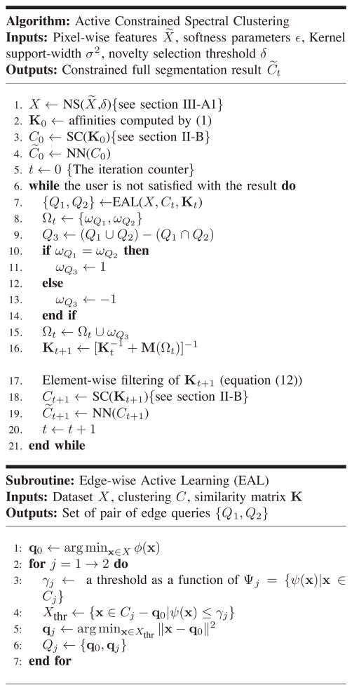
Here we explain the main parts of our proposed algorithm, Active Constrained Spectral Clustering. A pseudocode is shown in Figure 1. There are four subroutines in the main body of the algorithm: (1) novelty selection (NS: line 1) for subsampling the data (see section III-A1); (2) Spectral Clustering (SC: lines 3 and 18) (see section II-B); (3) nearest neighbors (NN: lines 4 and 19) for generalizing labels from a subset of pixels to all the pixels and (4) Edge-wise Active Learning (EAL: line 7) for querying a pair of edges (see section III-B).
Fig. 1.
The main algorithm and subroutine EAL explained in section III
The algorithm starts by subsampling the image and computing the initial similarity matrix K0. This subsampling is carried out to control the computational complexity of the iterations, as described below. Using K0 an initial segmentation result C̃0 will be obtained. If the result is not satisfactory, the algorithm enters the while-loop (an interactive human-computer active learning loop) on line 6. Within this loop, from line 7 to line 15, pairwise queries are selected and appropriate constraints are generated accordingly. We discuss our pairwise query selection method in the next subsection. Finally, the similarity matrix is updated to Kt+1 (the same as K̄ in section II-B) on line 16 and the constrained segmentation result C̃t+1 is obtained. This procedure is iteratively repeated until it converges to the user’s satisfaction.
In the remaining parts of this section, we first describe the computational methods employed to speed-up the spectral core method. Then the learning accelerator component of our algorithm is presented, that is the edge-wise active learning (EAL) subroutine.
A. Computational Speed-up Techniques
The algorithm described in section II-B is not practical to apply to large datasets, and in particular to typical digital images. This is mainly due to the costly eigen-decomposition of the Laplacian matrix. As mentioned before, there are several ways of combating this problem. In this work, we joined two approaches: (1) subsampling the data and (2) efficient numerical eigen-decomposition of the Laplacian matrix. These two methods are described in the following two sub-sections:
1) Sub-sampling
We simply reduce the size of the similarity matrix by subsampling the data, while trying to preserve as much information as possible. Novelty selection, introduced by Paiva and Tasdizen [26], is a greedy sampling approach aiming to select samples with low redundancy.
Suppose is the feature set of all the pixels in the image. We start from an empty subsample set, add the first point x̃1 and go through the remaining data points one by one. Each time, the minimum Euclidean distance between a candidate point and the already selected samples is computed and compared with a pre-specified threshold δ. The point will be added to the sample set only if the minimum distance is larger than δ, otherwise its nearest neighbor among the selected samples will be stored. Therefore the denser a region is, the more samples are generated around that area. Clearly for homogeneous regions the algorithm is equivalent to uniform sampling. For the rest of the paper, we denote X as the set of selected samples using this technique and also assume that |X| = n. Note that this technique has the computational complexity of O(nñ).Our segmentation algorithm runs on X to get a sparse set of labels C followed by generalization to the full set of labels C̃ by means of Nearest Neighbors (NN).
2) Numerical Eigen-decomposition
Numerical approaches are widely used to scale large eigen-decomposition problems. Orthogonal iteration4 is a generalization of the well-known power method to estimating multiple eigenvectors associated with the largest eigenvalues iteratively [10]. Specifically, since we work with two clusters, the goal is to estimate an orthonormal basis for the dominant 2-dimensional invariant subspace of the Laplacian L. Here we give a very brief description of the algorithm; more details together with pseudo-code are provided in Appendix B.
The algorithm is initialized with two orthonormal vectors. The following iterations can be summarized in two steps: the result of the last iteration is left-multiplied by Lq where q ≥ 1 is an integer parameter chosen according to the structure of L. Then we orthonormalize the resulting vectors using a Gram-Schmidt process. Iterations of this procedure have been shown to converge to the true dominant eigenvectors if the second and third eigenvalues are not equal. In Appendix B, we show that the number of operations required for this algorithm is linear with respect to n, and therefore it runs faster than the Lanczos and Nystrom methods mentioned earlier.
B. Edge-wise Active Learning (EAL)
As described, the goal in active learning is to minimize the number of queries required to obtain the desired segmentation outcome. We can achieve that by asking for feedback on samples about whose cluster assignments we are most uncertain [29]. Specifically, the sample with the largest uncertainty score is selected to be queried and correspondingly constrained, with the hope of decreasing total uncertainty of the segmentation.
Since we work with pairwise constraints, our query selection strategy is over pairs of samples or edges. This suggests linking a point with high uncertainty to another point with low uncertainty (or high certainty) and asking if they should be linked. In order to avoid being biased to the cluster of the high-confidence point, we also query the edge between the uncertain point and a high-confidence point in the other cluster.
Let us now clarify the notation used in Figure 1. Each edge Q connecting the points q1 and q2 is denoted by a set comprised of its end-points: Q = {q1, q2}. ωQ indicates the edge label over Q provided by the user: 1 if Q is specified as a must-link and −1 otherwise. Our active learning strategy aims to generate two edges Q1 = {q0, q1} and Q2 = {q0, q2} where the central point q0 has low confidence, whereas the other two points are highly certain samples assigned to different clusters.
The standard measure of uncertainty is entropy, which requires us to construct a probabilistic model for each cluster:
Probabilistic Modeling of the Clusters
To compute the assignment entropy at a given sample x ∈ X, we need to estimate the posterior probability that a sample belongs to a certain cluster given its features. Note that the posterior probability is computed based on a given clustering result C = {C1, C2}
| (5) |
The likelihood function p(x|x ∈ Ci) for each cluster i = 1, 2 can be estimated using kernel density estimation (KDE):
| (6a) |
| (6b) |
where k is the same kernel function as in (1). The class priors can also be computed empirically (P(x ∈ Ci) = P(Ci) = |Ci|/n, i = 1, 2), which results in the following class posterior probabilities:
| (7) |
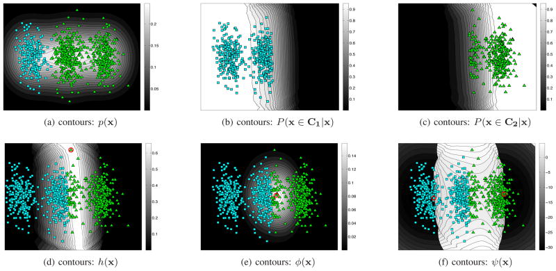
Note that in equations (5) and (7), , the evidence, is just a normalization constant. Figure 2 gives a simple 2-dimensional example used to illustrate the probabilistic concepts introduced here and also later in section III-B. In the first row, Figure 2a shows synthetic data generated by a mixture of three Gaussian components. The samples are colored according to the true clusters and displayed on top of the marginal density contours. Figures 2b and 2c show the two clusters resulting from an unconstrained spectral clustering, each of which is shown over its own posterior distribution contours computed by (7).
Fig. 2.
Illustrating probabilistic concepts of our approach: (a) three Gaussian components with different means and equal covariances used to generate the points that are displayed over contours of their marginal distribution. The points in each desired (gold-standard) cluster are shown in a different color and shapes; (b,c) the resulting groups after doing an unconstrained spectral clustering lying on contours of their corresponding posterior distribution; (d) the resulting groups shown together over contours of the posterior entropy h, with the encircled point as the one with the largest h; (e) the resulting groups over contours of the density weighted entropy ϕ, with the encircled point as the one with maximum ϕ (i.e. q0); (f) the resulting groups over contours of the inverse-density weighted entropy ψ, with the encircled points having the minimum ψ and shortest distance to q0 in each cluster (i.e. q1 and q2).
Finally the posterior entropy can be obtained using Shannon’s definition:
| (8) |
One problem is that entropy-based querying is not robust to low-evidence points (outliers), which does not lead to maximal affinity propagation (discussed in section IV-A). This fact is illustrated in figure 2d where the result of unconstrained spectral clustering is shown together with the contours of its posterior entropy. As can be seen, the entropy is independent of the evidence and is large everywhere close to the boundary between the clusters. Indeed, in this specific example, maximum entropy occurred in a low-evidence region.
Density-Weighted Entropy
One solution is to weight the entropies by marginal distributions to get a density-weighted scoring metric [29]:
| (9) |
where h(x) is defined in equation (8). The uncertain point q0 is selected by maximizing ϕ(x), which selects points with both high uncertainty and high evidence, and thus ignores outliers. Figure 2e shows contours of ϕ for our example, where the sample with the largest value is located in a crowded region close to the boundary.
Inverse-Density-Weighted Entropy
Similarly, using entropy by itself to find the high confidence end-points would suffer from outlier vulnerability (observe in Figure 2d that minimum entropy happens in low-density tails of each cluster). Again a weighting technique is used to make the metric more robust, but since here we encounter a minimization problem, we define an inverse-density-weighted entropy:
| (10) |
The behavior of this function is shown for our toy example in Figure 2f, where contours of ψ(x) are shown on a logarithmic scale. It can be observed that the lowest values occur in low-entropy high-density regions.
We chose the confident points to be the closest ones to q0 in a pool of samples with sufficiently high ψ (line 5 in EAL). Thresholding parameters are tuned based on statistical information about each cluster (line 3 in Figure 1). In Figure 2f, the encircled points are q1 and q2 selected with respect to q0 displayed in Figure 2e.
Finally, the edges Q1 and Q2 can be viewed as edges of an incomplete triangle. Label of the third edge Q3 can be easily inferred in a binary clustering (lines 9 through 15). By adding this additional label to the collection of constraints, the current iteration of query generation finishes.
The generated pairwise queries Q1, Q2 and Q3 are then labeled and used to update the similarity matrix by affinity propagation described in section II-C.
IV. Experimental Results
In this section, first we present some details about algorithm implementation, and then describe its performance as evaluated using the Berkeley segmentation dataset. We also report specifically on evaluation of our active learning strategy by comparing it to four different strategies.
A. Implementation Details
Some practical points regarding the affinity update process are discussed here. To analyze this process theoretically, we consider only one constraint ωij for simplicity. We rewrite the update equation in a linear form (using the matrix inversion lemma and after some simplifications) so that K̄ = KT(ωij). The transformation matrix T(ωij) can be described columnwise as:
| (11) |
where
Equation (11) implies that each column of the updated matrix is a modification of the corresponding column in the original affinity matrix. This modification is minimal for regions far away from xi and xj. Also observe that as ε grows, θt and hence the impact of the constraints, decreases.
The update shown in (11) suffers from the fact that there is no upper bound on the value of the modifications. As a result they may violate two key properties of the Gaussian assumption on the affinities in K̄; non-negativity of the elements, and the requirement that self-similarities should be equal to unity and greater than or equal to cross-similarities. In Lu and Carreira-Perpiñán’s work [17], a heuristic was introduced for shrinking all negative updated elements to zero. Here, we also imposed a heuristic for projecting values larger than one to unity. Specifically, we limit each element of the updated matrix k̄ij between zero and one as follows:
| (12) |
Another observation is that if both end-points of a constraint ωij are outliers, then the updates would be too small (kit, kjt ≪ 1, ∀ t ∈ {1, …, n}−{i, j}). Even if only one end-point is an outlier, the amount of propagation is limited. This is the reason why in our active learning strategy we avoided choosing outliers.
B. Results on Berkeley Segmentation Dataset
In order to test the performance of our algorithm, we first applied it to the Berkeley segmentation dataset [20]. We selected 55 images from both training and testing categories based on the existence of a meaningful object in each selected image that was not trivial to cluster using our core method. We use the Rand Index (RI) with respect to the gold-standard segmentation as a clustering metric:
with TP and TN true positive and true negative pixels with respect to the targeted object. Note that although the tasks of constraining and clustering are performed over the subsampled pixels, the accuracy is measured on the entire image.
To avoid subjectivity from a particular user and for ease of testing, we ran the evaluation reported here in a fully automated mode. In particular we substituted a perfect oracle for the user, represented by the program itself, which answered queries using the ground truth segmentation. The while-loop in the main algorithm (Figure 1) was thus replaced by a for-loop whose length was fixed to a sufficiently large number (here 500). After processing all 55 images we computed the average and standard deviation of RI across the images as a function of iteration index. With the computational acceleration described earlier, the algorithm ran quickly in MATLAB on a standard desktop with 12 GB of memory with no further optimization beyond the eigen-decomposition method described above. Computed time per iteration varied from 0.05 to 4 seconds with an average of 0.8 seconds and a standard deviation of 0.65 seconds.
To minimize the effect of particular choice of features, we used a very simple pixel-wise features, namely the spatial coordinates and the luminance intensities (d = 3), all normalized to unit variance.
Throughout this section we used the following parameter values chosen empirically: the threshold δ in the novelty selection algorithm was set to 0.2; the diagonal terms in Σ were set to 0.25 for both spatial features (normalized x- and y-coordinates) and to 0.5 for intensity; kernel values smaller than 5×10⁻² were shrunk to zero; and γj = min Ψj, j = 1, 2 in EAL. See Appendix B for details regarding the orthogonal iteration and the default values used there.
A nice property of our constrained spectral clustering algorithm is that it allows incorporation of the confidence of the labeler regarding the constraints they provide through the softness parameter ε (see equations 3). In real-world scenarios, we expect that during later stages of active learning, the labeler will be queried with more and more difficult edge queries and hence would have less confidence in their provided constraints. Mimicking such scenario, we introduce a dynamic parameter ε(t) where the labeler’s confidence diminishes with iteration index t. In this section, we present experimental results for two settings: (1) constant softness parameter, where we assume that the labeler/oracle confidence in their constraint information is constant, and (2) dynamic softness parameter, where we assume that the labeler’s confidence diminish with iteration.
1) Constant Softness Parameter
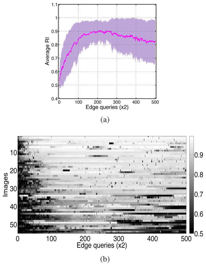
The softness parameter ε is fixed to a small constant, 10−5. The mean and standard deviation of clustering accuracy measured for all iterations are shown in Figure 3a. We recall that each iteration of the algorithm queries two edges, so that 500 iterations implies that 2×500 = 1000 edges have been labeled in total. The average RI starts from about 55% for the unconstrained segmentation and at its peak (around 2×200 labeled queries) achieves about 90% accuracy.
Fig. 3.
Results of running the algorithm with constant ε: (a) average and std RI versus different number of constraints; (b) the accuracy image: RI of segmenting individual images versus the iteration index
It can be observed that after getting about 2 × 250 constraints the average accuracy gradually starts decreasing. At the same time, the standard deviation also increased. This means that continued imposition of even correct constraints may cause accuracy reduction. We are observing a decrease in performance as labels are increased because at this point the learning algorithm is over-fitting the constraints. An accuracy image is shown in Figure 3b, which displays a matrix whose rows and columns correspond to RI of individual images and iteration index respectively. A dark region on the left part of this figure means that the unconstrained segmentation gives a poor result. Ideally the figure should uniformly get brighter as we move towards the right. In contrast, although for most of the images (rows) the accuracy is much higher than that at the start, as we scan to the right we see many black spots and dark regions confirming that the aforementioned decrease in the average accuracy is mainly due to sharp decreases in the accuracy of individual results after getting close to a perfect segmentation. Figure 4 illustrates how over-fitting can occur. The transition between the objects in natural images usually takes place smoothly. Consequently some object pixels near the boundary can have intensities similar to nearby background pixels as shown in Figure 4. At the same time, such pixels are the likeliest ones to be selected by EAL as the most uncertain point, especially when the current segmentation result is nearly perfect. Putting constraints in these cases can be misleading because it can easily push many background pixels into the segmented object. Note that in real settings, because active learning segmentation is interactive, the user will stop the iteration once almost perfect segmentation is met, which would thus avoid the over-fitting issues that usually occur in later iterations.
Fig. 4.
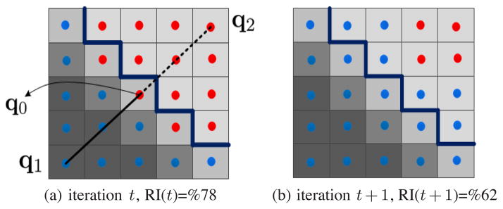
Illustration of a potential reason for fluctuating results. Blue and red pixels form two clusters and the thick dark blue boundary separates the correct segments. (a) The segmentation result at iteration t which is close to the ground-truth together with the constraints Ωt+1 including a must- (Solid edge) and cannot-link (dashed line). Observe that the central point q0 is an object pixel with features very similar to background. (b) The results after applying Ωt+1. Notice that many background pixels have been pushed into the object cluster and the accuracy is reduced RI(t)>RI(t + 1).
2) Dynamic Softness Parameter
In real interactive settings, the user can also incorporate their uncertainty in their labels through the softness parameter ε. Because, we are simulating the user labeling automatically, we make the softness parameter ε dynamic so that it increases (reflecting diminishing confidence) according to some schedule. This implies the algorithm will put less weight on the constraints as the iterations continue. Here we use a linear schedule for the softness parameter of the algorithm (t = 0 corresponds to the unconstrained initialization):
| (13) |
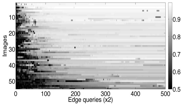
where ε0 is the minimum softness. We tried such linear schedules on the Berkeley dataset with ε0 = 10−5 and different values for the slope m. According to Figure 5a, which shows the average accuracies, using m = 10−4 yielded practically the same result as m = 0. Increasing m to 10−3 reduced the decrease in the average accuracy to some degree while setting it equal to 10−2 eliminated the decrease along with the fluctuations. Further increase in m caused the algorithm to become saturated prematurely before reaching an acceptably high accuracy. Figure 5b indicates that the value m = 10−2 outperformed others in terms of RI standard deviation too. An accuracy map of individual images in the dynamic case is shown for m = 10−2 in Figure 6, confirming the stabilizing effect of using a dynamic parameter. We observed that incorporating a dynamic schedule makes our constrained spectral clustering with active learning robust to over-fitting.
Fig. 5.

(a) Average and (b) standard deviation RI of trying different values for m in equation (13) (m = 10−4, 10−3, 10−2 and 10−1); average RI obtained by running the dynamic algorithm with m = 10−2 over (c) Cars and (d) People categories of INRIA image data set.
Fig. 6.
RI measurements for segmentation of individual images while using dynamic softness with a linear schedule and m = 10−2.
In order to investigate the generalization of the described dynamic algorithm, we ran it with the same set of parameter values mentioned above and with the best schedule understood from the results coming from the Berkeley data set (that is m = 10−2) on the Graz-02 image dataset [19], [25], categories of Cars and People. We chose 80 images from each category and applied our dynamic algorithm on them for 500 iterations. The resulting average and standard deviation RI are shown in Figures 5c and 5d implying that the results are very similar to what we got from the Berkeley data set.
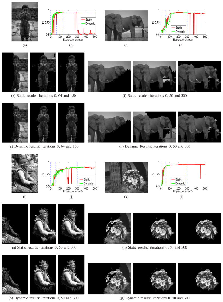
Figure 7 shows the results on four individual images. The first and fourth rows show the gray-scale original images and the RI accuracy plots. The dashed lines in the plots show the iterations from which the results have been selected to be displayed in the other rows: the second and fifth rows containing the static results, and the third and sixth rows showing the dynamic results (where a linear schedule with m = 10−2 was used). The selected iterations for all, except the child image are the same. They were chosen to show the initial, pre-convergence and post-convergence cases. In the first image, they were chosen such that the second phase coincides with a valley and the third happened before a permanent break in the static case.
Fig. 7.
Segmentation results of some iterations on four individual images: the first and fourth rows indicate the original gray-value images together with their corresponding RI plot for all iterations. The blue lines over these plots show the iterations whose results are selected to be displayed in other rows. The second and fifth rows show the static results, and the dynamic results are in the third and sixth rows.
Since the feature set used here is not descriptive enough, the initial unconstrained segmentations are far from the desired result, but, as expected, constraining them increases the accuracy. We observe that there are sharp valleys in the accuracy plots, especially in static cases. The valleys usually occur after convergence. In real settings, users would have terminated the iterations before they occur because they would have been already satisfied with the segmentation (see the plots in 7d, 7j, 7l). But some valleys occur in earlier iterations (see figure 7b). The algorithm was able to recover to high accuracy from these values most of the time.
In Figure 7 we can see that the boundary of clusters are not smooth and sometimes small isolated components appeared. These are the effects of generalization of the cluster assignments from a sparse set of labels to the full set that contains all the pixels. By decreasing the sampling threshold δ we may reduce this sampling effect at the expense of higher computational complexity.
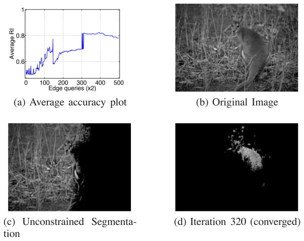
Finally, as Figure 6 implies, for a few images the algorithm did not converge to high accuracy in 500 iterations even when using dynamic softness. An example of such a failure is shown in Figure 8. This is likely caused when the features are too naive (note that we are only using intensity and the x, y location as features), thoroughly mixing up the clusters, so that restoring a small portion of all possible pairwise constraints to correct assignments cannot help discriminate the clusters [15].
Fig. 8.
One of the few images for which the algorithm failed to converge to a high accuracy.
C. Active Learning Evaluation
We evaluated our active learning strategy against four different scenarios explained below. The first three applies active learning strategies based on three simulated users (cases (i), (ii) and (iii)) and the segmentation is learned via our constrained spectral clustering approach. The fourth one is an alternative active learning strategy and constrained clustering proposed by Wang and Davidson [32] (case (iv)).
Random query selection: the query points q0, q1 and q2 are chosen randomly from the samples.
Object-oriented query selection: we simulate a smarter user who looks at the structure of the target object. Specifically, the user starts by putting cannot-links between interior and exterior points that are located close to the object’s border, and gradually moves to points further from the borders. Interior and exterior points themselves are must-linked separately.
Boundary-oriented query selection: We simulate another user behaving similar to our active learning strategy. The central point q0 is chosen randomly as a pixel on the current segmentation boundary and the other end-points, q1 and q2, are selected randomly from within a ball of a specific radius around q0.
Wang and Davidson’s method [32]: Their active learning strategy selects the best edge to query that minimizes the expected error. To perform constrained spectral clustering, they add must-links and cannot-links as additional constraints to the spectral clustering optimization formulation. All the parameters in this algorithm here are set to the recommended values given in the original work [32].
Cases (i), (ii) and (iii) are compared in Figure 9 against EAL in both static and dynamic modes. It shows that random querying increased the accuracy more slowly compared to our method, EAL, and also did not achieve the same accuracy. The object-oriented strategy improved the accuracy as rapidly as EAL during the first iterations, but totally failed before convergence. Note that for the images with small target objects, the number of possible constraints with this strategy was less than 2 × 500. Also querying based on (iii) produced very slow improvement in terms of the average RI.
Fig. 9.
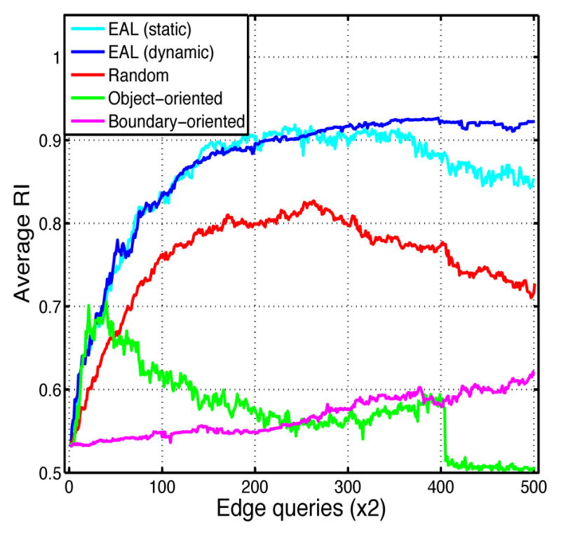
Comparing EAL ran with static affinity propagation (ε = 10−5) with three different query selection scenarios described as cases (i), (ii), (iii) in section IV-C, all of which ran with the sampling factor δ = 0.2.
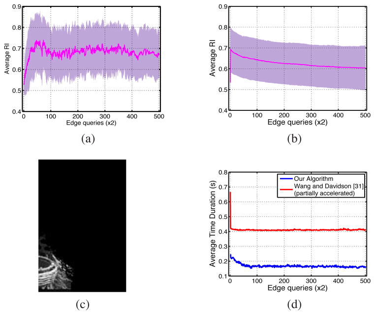
The active learning strategy in (iv) uses a different base constrained clustering algorithm. The numerical acceleration technique described in III-A2 cannot be directly applied to their method and therefore it is not computationally cheap enough to be applied to the same data used in the last section (obtained using δ = 0.2). Therefore we increased the sampling threshold to δ = 0.5 in order to reduce the number of samples and used it for comparison. The results are illustrated in Figures 10a and 10b. Note that in order to make Wang and Davidson’s algorithm comparable to ours we queried two pair-wise edges at each of its iterations. While our algorithm behaved similar to the case when δ was 0.2, the alternative active spectral clustering method increased the accuracy in early iterations but then failed to consider efficiently further constraints. This method was designed for general data and not ready for scaling to large data, such as images, unlike our method, EAL. Furthermore, [32] optimizes for expected error. Note that in images, typically there are more background pixels than foreground. We noticed empirically that the results of their algorithm tend to converge to unbalanced segmentations (see the individual segmentation example in Figure 10c for the old woman image shown in Figure 7i). Correctly classifying background tends to reduce the error. We investigated and found that their active learning strategy tends to select edge queries in the background region, rather than querying foreground or boundary information, leading to poorer segmentation performance. Our proposed active learning strategy, on the other hand, optimizes for uncertainty. This tends to pick points on image boundaries, which is important for image segmentation.
Fig. 10.
(a,b) the average and std RI of EAL and Wang and Davidson’s algorithm on a smaller dataset obtained by using δ = 0.5; (c) the segmentation result of Wang and Davidson’s algorithm [32] on the old woman image shown in Figure 7i picked from an iteration after convergence. Observe that it has converged to an unbalanced segmentation with low accuracy; (d) Average running time of Wang and Davidson’s constrained spectral clustering [32] and our algorithm ran with constant ε = 10−5
Since the cases (i), (ii) and (iii) all use our constrained clustering approach, their average running time for individual iterations are similar, removing the need for any comparison. Figure 10d shows that the average running time for case (iv) is almost twice as large as our algorithm in all iterations. This illustrates the speed improvement effect of our fast numerical eigen-decomposition.
V. Limitations
There are shortcomings that we did not eliminate in this work and which need further research. The major drawback of the algorithm is that it does not guarantee that all the constraints are satisfied. More specifically, the algorithm tends to strictly satisfy the most recent constraints and “forget” the earlier ones. If the algorithm could recall previous constraints, the instabilities we have observed would be less probable. One possible solution to this shortcoming is to re-emphasize the constraints while discretizing the labels in the spectral space (for example by doing constrained k-means [1]).
Another issue is related to the stabilization of the algorithm along the iterations (see section IV-B2): it is not always possible to design an efficient schedule for ε(t) automatically if labelers do not indicate their confidence in labeling.
Finally, we have used heuristics in order to restore some of the key characteristics of the updated affinity matrix K̄. Post-processing K̄ in equation (12) might weaken the effect of constraints by eliminating the information hidden in truncated values. An elegant solution could be obtained by defining a subspace of similarity matrices and projecting the updated affinity onto this group; however this is not a straightforward procedure. Klein et. al [15] post-processed the modified affinity matrix by computing the all-pair-shortest-paths using the updated values and substituting the result into the new matrix. This technique was useful for re-establishing the missing triangle inequality but cannot cope with negativity.
VI. Conclusion and Future Work
This work addresses the problem of constrained unsupervised segmentation. We have built a framework based on constrained spectral clustering with affinity propagation proposed by Lu and Carreira-Perpinán [17] to incorporate pairwise constraints in the form of must- or cannot-links. The main purpose is to accelerate the convergence to the user’s desirable segmentation by both directly reducing computational costs and also choosing edge queries between the most effective pairs of pixels. The former is performed by subsampling the input image and employing a numerical method to do the eigen-decomposition needed in spectral clustering, and the latter is addressed by devising an edge-wise active learning (EAL) technique to propose edge queries which will have the largest impact on the total uncertainty about the clustering assignment.
Performance of the algorithm is evaluated using 55 general images selected from the Berkeley segmentation dataset. The results showed that starting from a very poor, close to random unconstrained segmentation, the algorithm could approach the gold standard segmentation reasonably fast in comparison with random query selection and other simulated strategies. The major shortcomings of the algorithm include its violation of earlier constraints and instability along iterations. One reasonably effective solution developed to cope with the latter was to set up a monotonically increasing schedule for the softness parameter of the algorithm. This dynamic algorithm is also tested on two alternative data sets containing 80 images from the Cars and People categories of Graz-02 data set.
Our major future direction towards designing a constrained segmentation method will be on developing an algorithm with fewer heuristics while addressing the aforementioned shortcomings. Furthermore, there are other challenging issues to work on, such as batch-mode active learning, noisy oracles, and including variable labeling cost.
Acknowledgments
This project was supported by the National Institute of General Medical Sciences of the National Institutes of Health under grant number P41GM103545.
Biographies

Jamshid Sourati received his B.S. degree in Electrical Engineering at Sharif University of Technology, Tehran, in 2006 and is currently pursuing his Ph.D. degree in Electrical and Computer Engineering at Northeastern University, Boston. He is a member of Cognitive Systems Laboratory (CSL), Machine Learning (ML) and Biomedical Signal Processing, Imaging, Reasoning, and Learning (B-SPIRAL) groups at Northeastern. His main research interest includes active learning tied with spectral and probabilistic methods for doing semi-supervised and unsupervised data processing, combinatorial optimization and its usage in various machine learning applications and constrained density estimation/ clustering with non-parametric Bayesian models such as Dirichlet Process Mixture Models.

Deniz Erdogmus received BS degrees in EE and Mathematics in 1997, and MS in EE in 1999 from the Middle East Technical University, Ankara, Turkey. He received his PhD in ECE from the University of Florida in 2002, where he stayed as a postdoctoral research associate until 2004. He was an Assistant Professor of Biomedical Engineering at the Oregon Health and Science University until 2008. Then he joined Northeastern University, where he is currently an Associate Professor in the Electrical and Computer Engineering Department. His research focuses on statistical signal processing and machine learning with applications to contextual signal/image/data analysis with applications in cyberhuman systems including brain computer interfaces and technologies that collaboratively improve human performance. He has served as an associate editor and program committee member for a number of journals and conferences in these areas, including IEEE Signal Processing Letters, and the following IEEE Transactions: Signal Processing, Biomedical Engineering, and Neural Networks.

Jennifer G. Dy is an associate professor at the Department of Electrical and Computer Engineering, Northeastern University, Boston, MA, where she first joined the faculty in 2002. She received her M.S. and Ph.D. in 1997 and 2001 respectively from the School of Electrical and Computer Engineering, Purdue University, West Lafayette, IN, and her B.S. degree (Magna Cum Laude) from the Department of Electrical Engineering, University of the Philippines, in 1993. Her research is in machine learning, data mining and their application to biomedical imaging, health, security, science and engineering, with a particular focus on clustering, multiple clusterings, dimensionality reduction, feature selection and sparse methods, large margin classifiers, learning from the crowds and Bayesian nonparametric models. She received an NSF Career award in 2004. She serves as an associate editor for Machine Learning, an editorial board member for JMLR, organizing/senior/program committee member for ICML, ACM SIGKDD, AAAI, IJCAI, AISTATS and SIAM SDM, and program chair for SIAM SDM 2013.

Dana H. Brooks received the BA in English (‘72) from Temple University, and the BSEE (‘86), MSEE (‘88), and PhD (‘91) in Electrical Engineering from Northeastern University. He is a Professor of Electrical and Computer Engineering, Associate Director of the Center for Communications and Digital Signal Processing, co-founder of the Biomedical Signal Processing, Imaging, Reasoning, and Learning (B-SPIRAL) group, and PI of the BioMedical Imaging and Signal Processing Laboratory, at Northeastern, and a member of the Center for Integrative Biomedical Computing headquartered at University of Utah. He was a visiting professor during 1999–2000 at the Universitat Polit’ecnica de Catalunya in Barcelona, Spain, and visiting investigator at Memorial Sloan Kettering Cancer Center in New York, NY, in fall 2013 and at Massachusetts General Hospital’s Martinos Imaging Center in spring 2014. His research interests lie in application of statistical and digital signal and image processing to biomedical signal processing and medical and biological imaging, and in open-source software systems for these applications. Recent research projects include regularization for multimodal and dynamic biomedical inverse problems, fluoresence molecular and diffuse optical tomography, models of brain dynamics in relationship to imaging, inverse electrocardiography, modeling and optimization of non-invasive brain stimulation, and segmentation of lowcontrast and high-volume biomedical images.
Appendix A. Affinity Update
The basic derivations of the affinity matrix update can be found in [17]. Here we give a more detailed explanation of them.
For a constraint set Ω = ∪ (i,j) ωij, the non-zero elements of the sparse matrix M = M(Ω) appeared in (4), are as follows:
where the plus and minus signs in the off-diagonal terms are associated with cannot- and must-links respectively. This characterization implies that M(Ω) = Σωij∈ΩM(ωij). Therefore the update equation for Ω can be written as a sequential updates for the individual constraints:
where we associate each individual constraint with an index between 1 and |Ω|. Here we focus on one of the individual updates for a given ωij. From the structure of M(ωij), it is clear that there exists a permutation matrix such as P ∈ {0, 1}n×n that can make it block diagonal:
where . Also define
Now we show that if the update equation is written in terms of Mp and Kp, K̄ can be computed efficiently. To do this, first we define K̄p and relate it to K̄:
In this derivation, we used the orthogonality of permutation matrices (PTP = PPT = In). Using the Woodbury inversion identity, we can expand the equation for K̄p as:
| (14) |
Now it’s easy to verify the following key point regarding the inversion that appeared in the expanded format:
Plugging this result into equation (14) for computing K̄p yields:
The inversion here operates on a 2 × 2 matrix, and hence is straightforward to compute. Note that the condition number of this matrix for a given constraint ωij is proportional to
(plus when ωij ∈
 and minus when ωij ∈
 ). So one should be careful not to make ε2 too small such that the machine precision cannot handle inverting this ill-conditioned matrix. Moreover, the left and right matrix products, plus the necessary permutations for getting back to K̄ have the complexity of O(n), therefore the whole update can be done with O(n) operations.
Appendix B. Orthogonal Iteration
The eigendecomposition process is the main bottleneck in scaling up spectral clustering. Accurate estimation of all eigenvalues of L is very time consuming (O(n3)) and often not practical, especially when working with images. We employed the so-called orthogonal iteration method to numerically estimate the first two eigenvectors. This algorithm along with its extensions are discussed in many sources such as [10], [28]. Here we explain it in terms of our notations.
For any estimated eigenpair (v̂, λ̂) of a symmetric matrix L, where λ̂ is computed using the Rayleigh quotient, i.e. λ̂ = v̂TLv̂/v̂T v̂, the residual vector is defined as:
| (15) |
Provided that ||v̂||2 = 1 the eigenvalue estimation error is upper-bounded as below [28]:
| (16) |
Therefore the 2-norm of the residual vector can be used as a stopping criterion in iterative eigen-decomposition methods.
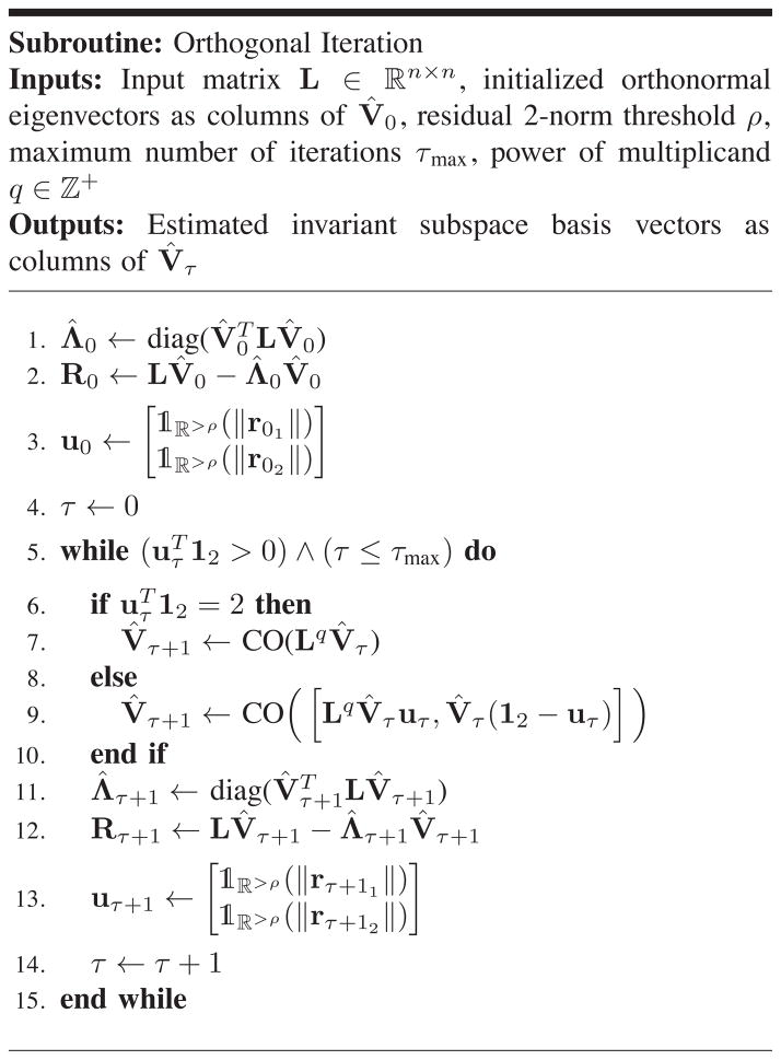
Figure 11 shows different steps in orthogonal iteration. Except for the initialization step (lines 1 through 3), each iteration (lines 4 to the end) consists of two phases: (1) updating the estimations and (2) computing the 2-norm of the residuals.
Fig. 11.
Orthogonal iteration subroutine used in Spectral Clustering (SC) to estimate eigenvectors associated with the two largest eigenvalues of the Laplacian matrix.
The algorithm is initialized by a random orthonormal matrix V̂0 ∈ ℝn×2. At each iteration τ = 0, …, τmax, in the first phase, either one or both columns of V̂τ are left-multiplied by the q’th power of L followed by orthonormalization to get V̂τ+1 (CO in lines 7 and 9 stands for column-orthonormalization). In our implementation we empirically fix q to 100. In the second phase, the Rayleigh quotient for each column of V̂τ+1 is computed (line 11) followed by calculating the residuals rτ+11 and rτ+12 as defined in (15) and forming the residual matrix Rτ+1. Finally computing the 2-norm of the residuals specifies if any of the iterating vectors has converged, so that it can stay fixed. The initialization only consists of phase (2) applied over the initial matrix V̂0.
Let us start from the second phase (lines 1–3 and 11–13). First, it implements equation (15) and then creates an indicator vector uτ+1 of length two whose components indicate whether the 2-norm of each individual column of Rτ+1 is greater than a pre-specified threshold ρ (fixed to 10−5 in our implementation). There are three possibilities for the element wise summation of this vector:
meaning that none of the columns in V̂τ+1 has converged and both of them will be updated during phase (1) of the next iteration (line 7, both columns of the estimation multiplied by Lq).
meaning that only one of the vectors has not yet converged, thus the algorithm keeps iterating on that, fixing the other one (line 9: just one column of the estimation multiplied by Lq).
meaning that both vectors have already converged, so that the loop can be terminated.
The convergence rate can be shown to be proportional to which is small when the data has two well-separated partitions. Moreover, the major operations of each iteration consist of the matrix-vector product and the orthonormalization process for which Gram-Schmidt algorithm is used. Since the input matrix is sparse, the product Lq V̂τ+1 has the complexity of order O(nq). Performing Gram-Schmidt process on the product result with size n ×2 takes O(n) operations [10]. Therefore complexity of the whole algorithm will be O(τmax.n(q + 1)) which is linear with respect to n.
Footnotes
In the context of machine learning, supervised and unsupervised methods are two extremes of a spectrum where the learning process is done with and without training labels respectively. Semi-supervised learning and constrained clustering are their user-interactive correspondences and sit closer towards each other along that spectrum.
In this paper, the terms affinity and similarity are used interchangeably.
More specifically, L, as defined above, is the normalized symmetric Laplacian matrix. According to Luxburg [18] there are other forms of Laplacian as well.
also known as subspace or staircase iteration.
Contributor Information
Jamshid Sourati, Email: sourati@ece.neu.edu.
Deniz Erdogmus, Email: erdogmus@ece.neu.edu.
Jennifer G. Dy, Email: jdy@ece.neu.edu.
Dana H. Brooks, Email: brooks@ece.neu.edu.
References
- 1.Basu S, Banjeree A, Mooney E, Banerjee A, Mooney RJ. Active Semi-Supervision for Pairwise Constrained Clustering. SIAM International Conference on Data Mining; 2004.pp. 333–344. [Google Scholar]
- 2.Boykov YY, Jolly MP. Interactive graph cuts for optimal boundary amp; region segmentation of objects in N-D images. IEEE International Conference on Computer Vision. 2001;1:105–112. [Google Scholar]
- 3.Ding L, Yilmaz A, Yan R. Interactive Image Segmentation Using Dirichlet Process Multiple-View Learning. IEEE Transactions on Image Processing. 2012;21(4):2119–2129. doi: 10.1109/TIP.2011.2181398. [DOI] [PubMed] [Google Scholar]
- 4.Eriksson AP, Olsson C, Kahl F. Normalized Cuts Revisited: A Reformulation for Segmentation with Linear Grouping Constraints. IEEE International Conference on Computer Vision; 2007.p. 18. [Google Scholar]
- 5.Falco AX, Udupa JK, Samarasekera S, Sharma S, Hirsch BE, de R, Lotufo A. User-steered image segmentation paradigms: live wire and live lane. Graphical Models Image Processing. 1998 Jul;60(4):233–260. [Google Scholar]
- 6.Fowlkes C, Belongie S, Chung F, Malik J. Spectral grouping using the Nystrom method. IEEE Transactions on Pattern Analysis and Machine Intelligence. 2004;26(2):214–225. doi: 10.1109/TPAMI.2004.1262185. [DOI] [PubMed] [Google Scholar]
- 7.Friedland G, Jantz K, Rojas R. SIOX: simple interactive object extraction in still images. IEEE International Symposium on Multimedia; 2005. [Google Scholar]
- 8.Gao J, Kosaka A, Kak A. Interactive color image segmentation editor driven by active contour model. International Conference on Image Processing. 1999;3:245–249. [Google Scholar]
- 9.Gao Y, Kikinis R, Bouix S, Shenton M, Tannenbaum A. A 3D interactive multi-object segmentation tool using local robust statistics driven active contours. Medical Image Analysis. 2012;16(6):1216– 1227. doi: 10.1016/j.media.2012.06.002. [DOI] [PMC free article] [PubMed] [Google Scholar]
- 10.Golub GH, Loan CFV. Matrix Computations. JHU Press; 1996. [Google Scholar]
- 11.Grady L. Random Walks for Image Segmentation. IEEE Transactions on Pattern Analysis and Machine Intelligence. 2006;28(11):1768– 1783. doi: 10.1109/TPAMI.2006.233. [DOI] [PubMed] [Google Scholar]
- 12.Hu YC, Grossberg MD, Wu A, Riaz N, Perez C, Mageras GS. Interactive semiautomatic contour delineation using statistical conditional random fields framework. Medical Physics. 2012;39(7):4547–4558. doi: 10.1118/1.4728979. [DOI] [PMC free article] [PubMed] [Google Scholar]
- 13.Hussein AA, Yang X. A statistical approach to interactive image segmentation. International Conference on Multimedia Technology; 2011.pp. 5260–5263. [Google Scholar]
- 14.Kang HW, Shin SY. Enhanced lane: interactive image segmentation by incremental path map construction. Graphical Models. 2002 Sep;64(5):282–303. [Google Scholar]
- 15.Klein D, Kamvar SD, Manning CD. From Instance-level Constraints to Space-Level Constraints: Making the Most of Prior Knowledge in Data Clustering. International Conference on Machine Learning; 2002.pp. 307–314. [Google Scholar]
- 16.Law YN, Lee HK, Ng MK, Yip AM. A Semisupervised Segmentation Model for Collections of Images. IEEE Transactions on Image Processing. 2012;21(6):2955–2968. doi: 10.1109/TIP.2012.2187670. [DOI] [PubMed] [Google Scholar]
- 17.Lu Z, Carreira-Perpiñán MA. Constrained Spectral Clustering Through Affinity Propagation. IEEE Conference on Computer Vision and Pattern Recognition; 2008.pp. 1–8. [Google Scholar]
- 18.Von Luxburg U. A tutorial on spectral clustering. Statistics and computing. 2007;17(4):395–416. [Google Scholar]
- 19.Marszalek M, Schmid C. Accurate Object Localization with Shape Masks. IEEE Conference on Computer Vision & Pattern Recognition; 2007. [Google Scholar]
- 20.Martin D, Fowlkes C, Tal D, Malik J. A database of human segmented natural images and its application to evaluating segmentation algorithms and measuring ecological statistics. International Conference in Computer Vision; 2001.pp. 416–423. [Google Scholar]
- 21.Mortensen EN, Barrett WA. Interactive Segmentation with Intelligent Scissors. Graphical Models and Image Processing. 1998 Sep;60(5):349–384. [Google Scholar]
- 22.Ng AY, Jordan MI, Weiss Y. On Spectral Clustering: Analysis and an algorithm. Advances in Neural Information Processing Systems; 2001.pp. 849–856. [Google Scholar]
- 23.Nguyen TNA, Cai J, Zhang J, Zheng J. Robust Interactive Image Segmentation Using Convex Active Contours. IEEE Transactions on Image Processing. 2012;21(8):3734–3743. doi: 10.1109/TIP.2012.2191566. [DOI] [PubMed] [Google Scholar]
- 24.Noma A, Graciano ABV, Cesar RM, Jr, Consularo LA, Bloch I. Interactive image segmentation by matching attributed relational graphs. Pattern Recognition. 2012;45(3):1159–1179. [Google Scholar]
- 25.Opelt A, Pinz A, Fussenegger M, Auer P. Generic Object Recognition with Boosting. IEEE Transactions on Pattern Recognition and Machine Intelligence. 2006 Mar;28(3) doi: 10.1109/TPAMI.2006.54. [DOI] [PubMed] [Google Scholar]
- 26.Paiva ARC, Tasdizen T. Fast semi-supervised image segmentation by novelty selection. IEEE International Conference on Acoustics Speech and Signal Processing; 2010.pp. 1054–1057. [Google Scholar]
- 27.Protiere A, Sapiro G. Interactive Image Segmentation via Adaptive Weighted Distances. IEEE Transactions on Image Processing. 2007;16(4):1046–1057. doi: 10.1109/tip.2007.891796. [DOI] [PubMed] [Google Scholar]
- 28.Saad Y. Numerical methods for large eigenvalue problems. Manchester University Press; 1992. [Google Scholar]
- 29.Settles B. Active Learning, Synthesis Lectures on Artificial Intelligence and Machine Learning. 2012;6(1):1–114. [Google Scholar]
- 30.Shi J, Malik J. Normalized cuts and image segmentation. IEEE Transactions on Pattern Analysis and Machine Intelligence. 2000 Aug;22(8):888–905. [Google Scholar]
- 31.Top A, Hamarneh G, Abugharbieh R. Active learning for interactive 3d image segmentation. International Conference on Medical Image Computing and Computer-assisted Intervention - Volume Part III; 2011; pp. 603–610. [DOI] [PubMed] [Google Scholar]
- 32.Wang X, Davidson I. Active spectral clustering. IEEE 10th International Conference on Data Mining; 2010.pp. 561–568. [Google Scholar]
- 33.Yu SX, Shi J. Grouping with Directed Relationship. Lecture Notes in Computer Science. 2001:283–291. [Google Scholar]
- 34.Zhang L, Ji Q. A Bayesian Network Model for Automatic and Interactive Image Segmentation. IEEE Transactions on Image Processing. 2011;20(9):2582–2593. doi: 10.1109/TIP.2011.2121080. [DOI] [PubMed] [Google Scholar]
- 35.Zou H, Zhou W, Zhang L, Wu C, Liu R, Jiao L. A new constrained spectral clustering for SAR image segmentation. Asian-Pacific Conference on Synthetic Aperture Radar; 2009.pp. 680–683. [Google Scholar]


