Imaging of Buried 3D Magnetic Rolled-up Nanomembranes

Abstract

Increasing performance and enabling novel functionalities of microelectronic devices, such as three-dimensional (3D) on-chip architectures in optics, electronics, and magnetics, calls for new approaches in both fabrication and characterization. Up to now, 3D magnetic architectures had mainly been studied by integral means without providing insight into local magnetic microstructures that determine the device performance. We prove a concept that allows for imaging magnetic domain patterns in buried 3D objects, for example, magnetic tubular architectures with multiple windings. The approach is based on utilizing the shadow contrast in transmission X-ray magnetic circular dichroism (XMCD) photoemission electron microscopy and correlating the observed 2D projection of the 3D magnetic domains with simulated XMCD patterns. That way, we are not only able to assess magnetic states but also monitor the field-driven evolution of the magnetic domain patterns in individual windings of buried magnetic rolled-up nanomembranes.

The urge to create energy efficient and ultrafast electronics led to the development of three-dimensional (3D) compact architectures in many disciplines including microelectronic chip design for optics¹⁻⁴ and magnetics.⁵⁻⁹ The application potential of those 3D systems have not been entirely explored due to the lack of a thorough fundamental understanding of the system’s response to external stimuli.^100−102 While engineering on-chip ring/tubular resonators provides unique opportunities to design three-dimensional optical logic and transmitter devices,⁴ magnetic tubular architectures reveal a significantly enhanced magnetoresistive/magnetoimpedance response,¹⁰ which may be applied in magnetoencephalography^11,12 and potentially faster memory devices.⁷ However, both fabrication and investigation of nonplanar high-quality three-dimensional architectures remains challenging.

Regarding the production of tubular architectures, electrochemical deposition in porous templates¹³⁻¹⁵ allows for fabricating submicrometer tubes but also leads to an unavoidable surface roughness.¹⁶ This is particularly crucial for magnetic materials due to intrinsic pinning of magnetic domain walls,¹⁶ which could lower the performance of future memory devices based on displacing magnetic domain walls in wires, such as the racetrack memory.¹⁷ An alternative fabrication approach of realizing 3D functional elements is strain-engineering and rolling up planar nanomembranes,^18,19 which provide similar film quality as of planar architectures^5,20,21 and an on-chip integretability combined with enhanced compactness.^5,22 The magnetization configuration of those tubular systems is commonly measured by integral means, such as ferromagnetic resonance,^6,20 anisotropic magentoresistance (MR)²³⁻²⁵ and cantilever magnetometry^26,27 measurements. The magnetic states can become rather complex due to the three-dimensionality of the architecture. For instance, six different states were proposed to explain the MR response of tubular magnetic architectures.^25,26 An experimental imaging of these magnetic textures is still lacking, though.

As the magnetic pattern determines the electrical response of the tubular elements, clear identification of magnetic states and monitoring their field- or current-driven transitions are crucial, particularly with respect to sensing¹² and memory⁷ applications. However, an essential aspect that has to be considered is the modification of physical properties of on-chip integrated functional elements due to encapsulation for the sake of protection. For instance, encapsulating magnetic nanostructures or thin nanomembranes results in a substantial change of the magnetic properties, including magnetic anisotropy energy and saturation magnetization, that further affects their magnetic response.²⁸ The actual performance of those functional elements can only be acquired by visualizing the magnetic states and their transition in buried architectures.

Whereas magnetization reversal and domain pattern evolution in buried planar architectures are successfully studied using well-established synchrotron methods, such as XPEEM²⁹ and MXTM,³⁰ microscopy on 3D magnetic structures is not yet accomplished. Pioneering works on imaging free-standing 3D magnetic objects rely on magnetic force microscopy,³¹ magnetooptical Kerr microscopy,^21,32 transmission XPEEM (T-PEEM)^33,34 and MXTM.²¹ While MXTM averages over all layers, ordinary XPEEM reveals no information about buried layers. Advancing these XMCD-based microscopies to visualize buried 3D magnetic architectures represents a milestone in investigating novel on-chip devices.

Here, we present an approach to retrieve information about the magnetization within three-dimensional buried magnetic layers utilizing the shadow contrast in T-XPEEM and exemplarily demonstrate the visualization of the magnetization configuration within magnetic 3D rolled-up nanomembranes with multiple windings (Figure 1a). The observed 2D projection of the domain patterns are correlated with those obtained by simulating the XMCD contrast in the shadow for an assumed magnetization. High-symmetry objects, such as tightly wound tubes, have simple magnetic configuration that are analytically defined. More complex geometries require to perform anterior micromagnetic simulations. In the particular case of a magnetic rolled-up membrane (Figure 1a), the shadow contrast consists of narrow stripes aligned along the tube axis, which is used to assign the magnetization orientation in a certain segment on the magnetic layer. Assuming a continuous distribution of the magnetization, the pattern can be expanded to reveal the magnetization configuration and reversal of the entire buried object.

Figure 1.

Utilizing the shadow contrast in transmission XPEEM to visualize buried magnetic domain patterns in 3D magnetic architectures such as magnetic rolled-up nanomembranes with multiple windings. (a) Schematic of projecting the magnetization vector field as a negative onto the planar substrate. XMCD signal is taken from experiment. The transparent nonmagnetic outer layer hides the actual magnetic domain patterns from direct observation. Signal contributions from various layers can be identified. (b) Fabrication of magnetic rolled-up nanomembranes: selective release of the magnetic/nonmagnetic heterostructure (Permalloy/InGaAs/GaAs) and rolling up into tubular architectures leads to either tightly wound tubes or loosely wound rolled-up nanomembranes as exemplarily shown by SEM (c). Scalar bars indicate 1 μm. (d) Energy profile scan around the nickel L₃ and L₂ absorption edges perpendicular to a rolled-up nanomembrane shown above. Intensity is shown in black–brown–white colorspace with white representing zero intensity. Energy scans for several regions are plotted in (e) and indicated in (d). No signal is acquired from the tube; the shadow contrast reveals an inverted signal. (f) Magnetic hysteresis loop of a rolled-up nanomembrane obtained by longitudinal magnetooptical Kerr effect magnetometry by applying an in-plane magnetic field at an angle of 45° with respect to the tube axis.

The peculiarity of nonplanar three-dimensional architectures when illuminating at a shallow angle is the emanation of both direct (ordinary) and indirect (shadow contrast) electrons with opposite XMCD signals.³⁴ However, photoelectrons excited in buried 3D magnetic architectures cannot escape the sample surface due to the capping layer and do not contribute to the XMCD signal directly. The corresponding shadow image represents a negative with an enhanced contrast because it does not only refer to the magnetization at the very surface (as in XPEEM) but also to the underlying “bulk” region. The projection further enlarges the spatial resolution, as it expands the magnetization pattern along the x-ray propagation direction, e.g. perpendicularly to the tube axis. In our case at an incidence angle of 74°, the shadow expands by a factor of 3.6, enhancing also the signal-to-noise ratio.

We applied rolled-up nanotechnology based on strain engineering^18,19 to fabricate tubular architectures out of 15 nm-thick soft-magnetic Permalloy (Ni₈₀Fe₂₀, Py) films on strained [In₃₃Ga₆₆As(5 nm)/GaAs(5.6 nm)] bilayers with a diameter of ≲3 μm (Figure 1b,c). In particular, the strained InGaAs/GaAs bilayer was epitaxially grown on top of an AlAs sacrificial layer prepared on semi-insulating single-crystal GaAs(001) wafers by molecular beam epitaxy (MBE). The strain had been optimized to achieve rolled-up tubes with a diameter of 600 nm after selective underetching of AlAs layer in hydrofluoric acid (HF).³⁵ To fabricate a 3D magnetic rolled-up nanomembrane, a 15 nm thick Py film capped with a 2 nm thick Al layer were deposited via direct current (dc) magnetron sputtering at room temperature (base pressure, 7 × 10^–8 mbar; Ar pressure, 10^–3 mbar) before selective release of the stack from the wafer. As the unstrained Py layer becomes thicker (up to 15 nm), the diameter increases linearly up to 3 μm. The rolling-up process led to tubular architectures with different compactness as exemplarily shown in SEM images taken under oblique illumination at the edge of the tube (Figure 1c). The focus of our work is set on buried magnetic film that resemble tightly wound tubes or loosely wound rolled-up nanomembranes with a spacer separation up to 400 nm (Figure 1c). The large separation allows for discriminating layers in transmission XPEEM, where the circular polarized X-ray beam penetrates through a magnetic object. The difference in intensity of left and right circular polarized transmitted X-ray beam causes different number of photoelectrons emanated upon interaction with a substrate. The resulting intensity distribution is a 2D projection of the magnetization pattern within the 3D object. Throughout the experiments, the X-ray beam hits the sample at 74° with respect to the surface normal and at 45° to the tube axis. Although the first angle is setup dependent, it turned out to be perfectly suited to image in transmission^33,34 with an enlarged image of the magnetic contrast along the incidence direction. The latter angle is chosen to discriminate the magnetization with both longitudinal and azimuthal alignment in a single experiment assuring time efficiency of the measurement. Figure 1d maps the photoelectron intensity perpendicularly to the tube axis (line profile indicated in the top panel) as a function of the X-ray photon energy around the Ni L₂ and L₃ absorption edges. Extracting the energy scans at different locations reveals a nonzero measurable signal in the shadow region (−7% of the signal of the extended Py film) (Figure 1e). Thus, the magnetic signal acquired by T-XPEEM represents a negative of the magnetic domain pattern in the object. Furthermore, we emphasize that the signal directly measured on the tube is negligible and cannot be used for visualization of buried 3D objects. Longitudinal magnetooptical Kerr effect magnetometry was applied to investigate integral magnetic properties of the samples by exposing it to an in-plane magnetic field applied at 45° with respect to the tube axis (Figure 1f). By focusing the laser beam on the tube, the hysteresis loop was measured revealing a coercive field of (7 ± 1) Oe. Please note that only the top part of the tube within the light penetration depth (∼20 nm) contributes to the acquired signal.²¹ The two small kinks in the normalized Kerr rotation angle θ/θ_s originate from the surrounding planar film, which was confirmed by defocusing the laser beam to enlarge the film contribution to the Kerr signal.

We first demonstrate the approach by determining the magnetization pattern in a tightly rolled-up tube. Balhorn et al.⁶ showed by ferromagnetic resonance spectroscopy that tightly rolled-up Py nanomembranes behave like closed tubes due to magnetostatic coupling between adjacent windings. In this respect, basic spin configuration including azimuthal, longitudinal, and onion states are considered. The corresponding shadow contrast of these states is shown in Figure 2. The magnetization component along the propagation direction of the X-ray beam, namely 45°, is shaded in blue/red with white referring to a component perpendicular to the X-ray beam. The dashed–dotted lines enclose the shadow region of the tube located at the top. In contrast to Figure 1, the magnetization is projected onto a uniformly magnetized planar Py film. The homogeneously changing signal refers to layers with same magnetization configuration. In order to identify the corresponding magnetization patterns, we calculate the XMCD contrast in the shadow region.

Figure 2.

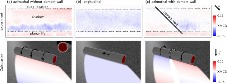
Comparison of the experimental XMCD data and shadow contrast simulation of (a) an azimuthally and (b) a longitudinally magnetized state (orientation of the magnetic moments is indicated by arrows) within a hollow magnetic tube. X-ray beam hits the tube at 45° with respect to the tube axis and 16° with respect to the substrate and projects the shadow onto a uniformly magnetized planar Py film. The magnetization component along the beam propagation is depicted in blue–red colorspace. Dashed–dotted lines enclose the shadow region of the tube with one winding. (c) An azimuthal state with a 180° domain wall domain wall perpendicular to the tube axis (double line).

The simulated contrast is obtained by taking the magnetization-dependent absorption of a circular polarized X-ray beam through a magnetic tube into account. The transmitted intensity of left and right circular polarized light reads I± = exp(−μ_±d) with the helicity-dependent absorption coefficient μ_± and the penetration depth d defined at each point of the tube. In case of Permalloy, the absorption coefficient may be approximated in first order as μ_± = μ_±^Fe[(a_Fe in Py)/(a_Fe)] + μ_±[(a_Ni in Py)/(a_Ni)] with the atomic density a. The individual absorption coefficients are estimated based on the work of Stöhr³⁶ (e.g., μ₊^Fe ≈ 1 μm^–1, μ_– ≈ 5 μm^–1, μ₊^Ni ≈ 3 μm^–1 at Fe L₃ absorption edge). Furthermore, the effective absorption is obtained by linear interpolation between μ_– and μ₊ with the scalar product of magnetization and X-ray propagation direction and scaled by the X-ray polarization degree. The magnetization field is analytically defined on a tube assuming a uniform distribution like longitudinal or azimuthal magnetization alignment. The accordingly defined intensity at each point j on the tube is multiplied along the X-ray propagation direction [I_± = exp(−∑_jμ₊d^(j))] and projected onto a plane representing the substrate.

From the comparison between experimental and simulated data, we identify states with azimuthal (Figure 2a) and longitudinal (Figure 2b) magnetization. As the X-ray beam hits the sample at 45° with respect to the tube axis, 180° domain walls perpendicular to the tube axis are projected under 45° in the shadow contrast. XMCD signals from overlapping regions with opposite magnetization orientation close to a domain wall cancel out each other and form in case of azimuthal orientation an elliptical region with zero XMCD contrast aligned along the beam propagation direction (Figure 2c). The good correspondence between experiment and simulation suggests that indeed tightly wound rolled-up nanomembranes with multiple windings can be treated as a hollow tube⁶ with a commensurable domain pattern throughout all windings driven by the magnetostatic interaction.

After successful visualization of these basic configurations, we further focus on a rolled-up nanomembrane with loosely wound layers that are separated by 180 to 270 nm, as revealed by the shadow contrast in qualitative agreement with SEM (Figure 1c). The corresponding XMCD signal of the object consists of narrow stripes aligned along the tube axis, which refer to the magnetic contrast originating from each winding. This assumption was verified by imaging with linear polarized light showing at the same location dark lines due to an effectively varying thickness. Applying an external magnetic field reveals an independent switching behavior of those stripes (Figure 3). The sample was initially saturated by applying an in-plane magnetic field larger than the switching field and sequentially exposed to increasing negative fields. As the shadow contrast is analyzed on top of a uniformly magnetized planar Py film, an additional but nondisturbing offset has to be considered. The central shadow region refers to layers that experience mainly perpendicular magnetic field components. Hence, contrast changes appear at larger fields. Contrary, the contrast at the edge of a winding fades and reverses at field values (−12∼−16 Oe) similar to those obtained by magnetooptical Kerr effect magnetometry (Figure 1f). The larger XMCD signal originating from the edge of each winding allows for reconstructing more complex magnetization configurations within the 3D magnetic architectures. The dependence of the magnetization reversal on the local magnetization orientation (domains) emphasizes the importance of layer specific imaging of individual windings. We chose three cuts through the loosely wound rolled-up nanomembrane (sections A, B, and C) and plot the magnetization orientation at each winding at these cuts as shown in the corresponding schematic 3D images in panels a–c of Figure 3. Stacking multiple line profiles along the tube axis enables us to assess the magnetization configuration within the 3D magnetic architecture. Our observation hints for a continuous domain pattern in the nanomembrane with oblique domain walls, thus appearing at different locations along the tube axis in each winding.

Figure 3.

Layer-specific imaging of buried three-dimensional magnetic rolled-up nanomembrane with multiple windings using T-XPEEM. The distinction between signals of different windings is accomplished as the absorption at the edges of the windings is pronounced (indicated by dashed–dotted lines). Location of the assigned windings coincided with that obtained by illuminating with linear polarized light due to varying penetration depth. (a–c) XMCD contrast at various external in-plane magnetic fields applied at 45° with respect to the tube axis, after saturating at 30 Oe. The magnetization is projected onto the uniformly magnetized planar film that switches already at −2 Oe. The magnetization at each winding can be reconstructed from the shadow contrast as shown for different line profiles (A, B, and C) and reassembled along the tube axis. (d) Line profiles along the tube, that is, of winding 3, provide insight into the magnetic field-driven evolution, including the distinction between domain wall displacement along or perpendicular to the tube axis (indicated by black arrow).

A more quantitative analysis of the magnetization including domain wall displacement during magnetization reversal is done by extracting the line profile of each winding along the tube axis, exemplarily shown for winding 3 in Figure 3d. The transition region in Figure 3d marked by brown and green arrows for external magnetic fields of −12 and −14 Oe, respectively, refer to the magnetic domain walls indicated by solid double lines in Figure 3a,b. The dashed double lines in Figure 3b represent for illustration the domain wall position at −12 Oe. Analyzing the XMCD signal of the top and bottom part of winding 3 reveals a displacement perpendicular to and along the tube axis, respectively. Assuming a continuous pattern, such a change may be assigned to a combination of domain wall translation and rotation, which is likely to occur in soft-magnetic materials. Moreover, the similarity of the magnetic pattern in Figure 3a–c to Figure 2c suggests an azimuthal or slightly tilted magnetization in the inner winding, whose energetically unfavored domain decreases in size by magnetization rotation and domain wall displacement.

In conclusion, we fabricated magnetic rolled-up nanomembranes of various tightness and retrieved information about the magnetization configuration within these buried three-dimensional magnetic architectures by means of transmission XPEEM. We verified the assumption of magnetostatically coupled layers for tightly wound tubes that lead to longitudinal or azimuthal alignment of the magnetization. Loosely wound rolled-up nanomembranes reveal continuous domain pattern in the nanomembrane with oblique domain walls. Our new approach provides further means to follow the magnetization reversal in each winding of a magnetic rolled-up architectures, which had not been accessible before. Because of the measurement of a single 2D projection of a 3D magnetization texture, merely highly symmetric objects with multiple magnetic layers possessing continuous magnetic domain patterns may be studied with the present approach. In this work, we assumed specific magnetic states to simulate the XMCD contrast, which was possible due to the high symmetry of the investigated architectures. In order to visualize and identify more complex 3D magnetic textures, the XMCD contrast has to be simulated using the magnetization obtained by anterior micromagnetic simulations. Our work represents the first important step toward the realization of magnetic soft X-ray computed tomography for investigating complex magnetic domain patterns in 3D architectures.

The authors declare no competing financial interest.

References

- Sherwood-Droz N.; Lipson M. Opt. Express 2011, 19, 17758–17765. [DOI] [PubMed] [Google Scholar]
- Bianucci P.; Mukherjee S.; Dastjerdi M. H. T.; Poole P. J.; Mi Z. Appl. Phys. Lett. 2012, 101, 031104. [Google Scholar]
- Bessette J. T.; Ahn D. Opt. Express 2013, 21, 13580–13591. [DOI] [PubMed] [Google Scholar]
- Böttner S.; Li S.; Jorgensen M. R.; Schmidt O. G. Appl. Phys. Lett. 2013, 102, 251119. [Google Scholar]
- Smith E. J.; Xi W.; Makarov D.; Monch I.; Harazim S.; Bolanos Quinones V. A.; Schmidt C. K.; Mei Y.; Sanchez S.; Schmidt O. G. Lab Chip 2012, 12, 1917–1931. [DOI] [PubMed] [Google Scholar]
- Balhorn F.; Jeni S.; Hansen W.; Heitmann D.; Mendach S. Appl. Phys. Lett. 2012, 100, 222402. [Google Scholar]
- Yan M.; Kákay A.; Gliga S.; Hertel R. Phys. Rev. Lett. 2010, 104, 057201. [DOI] [PubMed] [Google Scholar]
- Otalora J. A.; Lopez-Lopez J. A.; Vargas P.; Landeros P. Appl. Phys. Lett. 2012, 100, 072407. [Google Scholar]
- Yan M.; Andreas C.; Kákay A.; García-Sánchez F.; Hertel R. Appl. Phys. Lett. 2012, 100, 252401. [Google Scholar]
- Bermúdez Ureña E.; Mei Y. F.; Coric E.; Makarov D.; Albrecht M.; Schmidt O. G. J. Phys. D: Appl. Phys. 2009, 42, 055001. [Google Scholar]
- Hertel R. SPIN 2013, 03, 1340009. [Google Scholar]
- Mellem D.; Toedt J. N.; Balhorn F.; Mansfeld S.; Hansen W.; Mendach S. SPIN 2013, 03, 1340007. [Google Scholar]
- Vázquez M. J. Magn. Magn. Mater. 2001, 226–230Part 1693–699. [Google Scholar]
- Liu L.; Ioannides A. A.; Streit M. Brain Topogr. 1999, 11, 291–303. [DOI] [PubMed] [Google Scholar]
- Dumas T.; Dubal S.; Attal Y.; Chupin M.; Jouvent R.; Morel S.; George N. PLoS One 2013, 8, e74145. [DOI] [PMC free article] [PubMed] [Google Scholar]
- Che G.; Lakshmi B. B.; Fisher E. R.; Martin C. R. Nature (London) 1998, 393, 346–349. [Google Scholar]
- Nielsch K.; Wehrspohn R. B.; Barthel J.; Kirschner J.; Gösele U.; Fischer S. F.; Kronmüller H. Appl. Phys. Lett. 2001, 79, 1360–1362. [Google Scholar]
- Nielsch K.; Choi J.; Schwirn K.; Wehrspohn R. B.; Gösele U. Nano Lett. 2002, 2, 677–680. [Google Scholar]
- Biziere N.; Gatel C.; Lassalle-Balier R.; Clochard M. C.; Wegrowe J. E.; Snoeck E. Nano Lett. 2013, 13, 2053–2057. [DOI] [PMC free article] [PubMed] [Google Scholar]
- Parkin S. S. P.; Hayashi M.; Thomas L. Science 2008, 320, 190. [DOI] [PubMed] [Google Scholar]
- Prinz V. Y.; Seleznev V. A.; Gutakovsky A. K.; Chehovskiy A. V.; Preobrazhenskii V. V.; Putyato M. A.; Gavrilova T. A. Physica E 2000, 6, 828. [Google Scholar]
- Schmidt O. G.; Eberl K. Nature (London) 2001, 410, 168. [DOI] [PubMed] [Google Scholar]
- Balhorn F.; Mansfeld S.; Krohn A.; Topp J.; Hansen W.; Heitmann D.; Mendach S. Phys. Rev. Lett. 2010, 104, 037205. [DOI] [PubMed] [Google Scholar]
- Streubel R.; Lee J.; Makarov D.; Im M.-Y.; Karnaushenko D.; Han L.; Schäfer R.; Fischer P.; Kim S.-K.; Schmidt O. G. Adv. Mater. 2014, 26, 316–323. [DOI] [PubMed] [Google Scholar]
- Bof Bufon C. C.; Espinoza J. D. A.; Thurmer D. J.; Bauer M.; Deneke C.; Zschieschang U.; Klauk H.; Schmidt O. G. Nano Lett. 2011, 11, 3727. [DOI] [PubMed] [Google Scholar]
- Mönch I.; Makarov D.; Koseva R.; Baraban L.; Karnaushenko D.; Kaiser C.; Arndt K.-F.; Schmidt O. G. ACS Nano 2011, 5, 7436. [DOI] [PubMed] [Google Scholar]
- Müller C.; Bof Bufon C. C.; Navarro-Fuentes M. E.; Makarov D.; Mosca D. H.; Schmidt O. G. Appl. Phys. Lett. 2012, 100, 022409. [Google Scholar]
- Rüffer D.; Huber R.; Berberich P.; Albert S.; Russo-Averchi E.; Heiss M.; Arbiol J.; Fontcuberta i Morral A.; Grundler D. Nanoscale 2012, 4, 4989–4995. [DOI] [PubMed] [Google Scholar]
- Weber D. P.; Rüffer D.; Buchter A.; Xue F.; Russo-Averchi E.; Huber R.; Berberich P.; Arbiol J.; Fontcuberta i Morral A.; Grundler D.; Poggio M. Nano Lett. 2012, 12, 6139–6144. [DOI] [PubMed] [Google Scholar]
- Buchter A.; et al. Phys. Rev. Lett. 2013, 111, 067202. [DOI] [PubMed] [Google Scholar]
- Karnaushenko D.; Makarov D.; Yan C.; Streubel R.; Schmidt O. G. Adv. Mater. 2012, 24, 4518–4522. [DOI] [PubMed] [Google Scholar]
- Kronast F.; Ovsyannikov R.; Kaiser A.; Wiemann C.; Yang S.-H.; Bürgler D. E.; Schreiber R.; Salmassi F.; Fischer P.; Dürr H. A.; Schneider C. M.; Eberhardt W.; Fadley C. S. Appl. Phys. Lett. 2008, 93, 243116. [Google Scholar]
- Fischer P.; Kim D.-H.; Chao W.; Liddle E. H.; Anderson J. A.; Attwood D. T. Mater. Today 2006, 9, 26. [Google Scholar]
- Zarpellon J.; Jurca H. F.; Varalda J.; Deranlot C.; George J. M.; Martins M. D.; Parreiras S. O.; Muller C.; Mosca D. H. RSC Adv. 2014, 4, 8410–8414. [Google Scholar]
- Streubel R.; Makarov D.; Lee J.; Müller C.; Melzer M.; Schäfer R.; Bof Bufon C. C.; Kim S.-K.; Schmidt O. G. SPIN 2013, 03, 1340001. [Google Scholar]
- Kimling J.; Kronast F.; Martens S.; Böhnert T.; Martens M.; Herrero-Albillos J.; Tati-Bismaths L.; Merkt U.; Nielsch K.; Meier G. Phys. Rev. B 2011, 84, 174406. [Google Scholar]
- Streubel R.; Kravchuk V. P.; Sheka D. D.; Makarov D.; Kronast F.; Schmidt O. G.; Gaididei Y. Appl. Phys. Lett. 2012, 101, 132419. [DOI] [PubMed] [Google Scholar]
- Streubel R.; Thurmer D. J.; Makarov D.; Kronast F.; Kosub T.; Kravchuk V.; Sheka D. D.; Gaididei Y.; Schäfer R.; Schmidt O. G. Nano Lett. 2012, 12, 3961–3966. [DOI] [PubMed] [Google Scholar]
- Stöhr J. J. Electron. Spectrosc. Relat. Phenom. 1995, 75, 253–272. [Google Scholar]