

Abstract
High density diffuse optical tomography (HD-DOT) is a noninvasive neuroimaging modality with moderate spatial resolution and localization accuracy. Due to portability and wear-ability advantages, HD-DOT has the potential to be used in populations that are not amenable to functional magnetic resonance imaging (fMRI), such as hospitalized patients and young children. However, whereas the use of event-related stimuli designs, general linear model (GLM) analysis, and imaging statistics are standardized and routine with fMRI, such tools are not yet common practice in HD-DOT. In this paper we adapt and optimize fundamental elements of fMRI analysis for application to HD-DOT. We show the use of event-related protocols and GLM de-convolution analysis in un-mixing multi-stimuli event-related HD-DOT data. Statistical parametric mapping (SPM) in the framework of a general linear model is developed considering the temporal and spatial characteristics of HD- DOT data. The statistical analysis utilizes a random field noise model that incorporates estimates of the local temporal and spatial correlations of the GLM residuals. The multiple-comparison problem is addressed using a cluster analysis based on non-stationary Gaussian random field theory. These analysis tools provide access to a wide range of experimental designs necessary for the study of the complex brain functions. In addition, they provide a foundation for understanding and interpreting HD-DOT results with quantitative estimates for the statistical significance of detected activation foci.
Keywords: Diffuse optical tomography, General linear model, Statistical parametric mapping, Non-stationary cluster analysis
1. Introduction
With recent improvements in spatial resolution and brain specificity, along with the advantages of non- ionizing portable and wearable technology, high density diffuse optical tomography (HD-DOT) has become a promising neuroimaging modality for translation to clinical settings and cognitive studies in child brain development (Bluestone et al., 2001; Boas et al., 2004a; Boas et al., 2004b; Eggebrecht et al., 2012; Gibson et al., 2006; Gibson et al., 2005; Habermehl et al., 2012; Joseph et al., 2006; White and Culver, 2010a, b; Zeff et al., 2007). However, thus far HD-DOT reports have lacked event related designs and accurate statistical tools that are common to fMRI and crucial for imaging complex cognitive processes. In this work we focus on developing these analytical tools for HD-DOT. To validate the methods we acquired and analyzed event- related data in several healthy adult volunteers.
In order to extract the brain response to a given task using simple block averaging, task blocks need to be well separated in time (Bandettini et al., 1993; Blamire et al., 1992; Fransson et al., 1999). Blocked experimental designs suffer from predictable task timing and often lead to bored subjects and difficulties in maintenance of attention to task. Rapid “event-related” designs provide faster and more complex naturalistic paradigms (Friston et al., 1995). Developed within the statistical framework of a general linear model (GLM), event- related designs incorporate linear models of the response function into the analysis of time-series data, and enable un-mixing of the response to fast and event-related stimuli (Clark et al., 1997; Dale and Buckner, 1997; Friston et al., 1998; Josephs et al., 1997; Zarahn et al., 1997).
While some papers have implemented selected portions of statistical parametric mapping (SPM) techniques in the framework of GLM, none have done so in a comprehensive manner. For instance, some near infrared spectroscopy (NIRS) studies have implemented GLM to de-convolve overlapping responses (Abdelnour and Huppert, 2009; Ciftci et al., 2008; Cohen-Adad et al., 2007; Hu et al., 2010; Koh et al., 2007; Plichta et al., 2007; Plichta et al., 2006; Schroeter et al., 2004; Ye et al., 2009; Zhang et al., 2005). Some have evaluated Bonferroni corrections to the multiple comparison problem when setting thresholds for statistical significance (Hu et al., 2010; Plichta et al., 2007; Plichta et al., 2006), and some have implemented sophisticated SPM approaches with special considerations for spatially interpolated NIRS data (Ye et al., 2009). However these NIRS studies have not addressed HD-DOT data and imaging.
HD-DOT uses a dense array of optodes (compared to NIRS) which results in higher spatial resolution and its overlapping measurements results in spatially smoother data. With a forward model that describes the light propagation in the underlying tissue, HD-DOT reconstructs three-dimensional images of hemodynamic activity (Boas and Dale, 2005; Boas et al., 2004b; Custo et al., 2010; Eggebrecht et al., 2012; Heiskala et al., 2009; Koch et al., 2010; Zeff et al., 2007). Recently with a quantitative voxel-wise comparison against fMRI, it is shown that this technique can provide lateral resolution at the gyral-level and localization errors on the order of ∼5 mm (Eggebrecht et al., 2012). With these advances, HD-DOT comes closer to representing dense and continuous imaging fields and closer to resembling fMRI data (Eggebrecht et al., 2012; Habermehl et al., 2012). The improved image quality in turn motivates the use of fMRI based statistical approaches. Here we adapt statistical methods from standard fMRI analyses and evaluate the underlying assumptions in the context of HD-DOT imaging. In particular we evaluate local temporal and spatial autocorrelation structures of random fields from the residuals of a GLM. We implement a cluster analysis based on random field theory (RFT) to control the false positive rate in the statistical maps. To account for the potential spatial variance in the HD- DOT point spread function we use a non-stationary RFT approach
The body of this paper is arranged as follows: We begin by describing the data acquisition including the imaging array, subjects, and experimental designs. We then outline the preprocessing, and SPM procedure including; linear modeling of data, dealing with the temporal autocorrelations, and addressing the multiple comparison problem. We then present empirical in vivo results of functional event-related HD-DOT data acquired during visual activation in human adults. Finally we evaluate the performance of the GLM-SPM tools.
2. Methods
2.1. Subjects and experimental protocol
Six healthy right-handed subjects (age range: 17-30 years) were scanned. The research was approved by the Human Research Protection Office at Washington University School of Medicine. Subjects were seated in an adjustable chair in a sound-isolated room facing a 19-inch LCD screen at a viewing distance of 75 cm. All measurements were done with a continuous wave high-density DOT system. The imaging cap with 24 sources (flashing 750 nm and 850 nm LEDs) and 28 detectors was placed on the back of subject's head. For more details on the HD-DOT instrumentation see references (Eggebrecht et al., 2012; Zeff et al., 2007). The visual stimulus consisted of left and right flickering checkerboard wedges (flickering at 10 Hz), presented in a counterbalanced random order. The block design consisted of 10 blocks (5 left, 5 right) with an inter stimulus interval of 30 s. In the event design 15 left and 15 right stimuli were presented with inter stimulus intervals that were randomly distributed between 2-15 s. In both designs stimuli duration was 5s. There was a 30 second long fixation at the beginning of stimulus presentation. All subjects had been previously scanned with MRI (Siemens Trio (Erlangen, Germany) 3T scanner) for another study. Their anatomical T1-weighted MPRAGE (echo time (TE) = 3.13 ms, repetition time (TR) = 2400 ms, flip angle = 8°, 1 × 1 × 1 mm isotropic voxels) and T2- weighted (TE = 84 ms, flip angle = 120°, 1 × 1 × 4 mm voxels) images were used to generate subject-specific head models.
2.2. HD-DOT preprocessing
Raw detector data were decoded to source-detector pair data, and converted to log-ratio to mean values. The data then were band-pass filtered (0.02 Hz - 0.25 Hz) to remove long-term trends and pulse artifacts. All signals from the first-nearest neighbor channels were averaged to create a measure of the superficial hemodynamics. This nuisance signal was removed by linear regression from all channels. Additionally, data were down-sampled to 1 Hz. We used the subjects' T1 and T2 weighted images to segment their heads into five putative different tissue types, including scalp/skin, skull, CSF, white, and gray matter and created the subjects' head meshes (Eggebrecht et al., 2012). Light propagation inside the mesh was modeled using the diffusion approximation and a sensitivity matrix was generated using the finite-element modeling software (NIRFAST). The sensitivity matrix was inverted and smoothed with a Gaussian kernel, and used to reconstruct absorption coefficient changes for each wavelength (750 nm and 850 nm). The field of view (FOV) for a typical subject was a cube containing 26×41×69 voxels, covering occipital cortex, with isometric voxel size of 2×2×2 mm3. Relative changes in the concentrations of oxygenated (HbO), deoxygenated (HbR), and total hemoglobin (HbT) were obtained from the absorption coefficient changes by the spectral decomposition of the extinction coefficients of HbO and HbR at these two wavelengths (Fig.1).
Fig. 1.
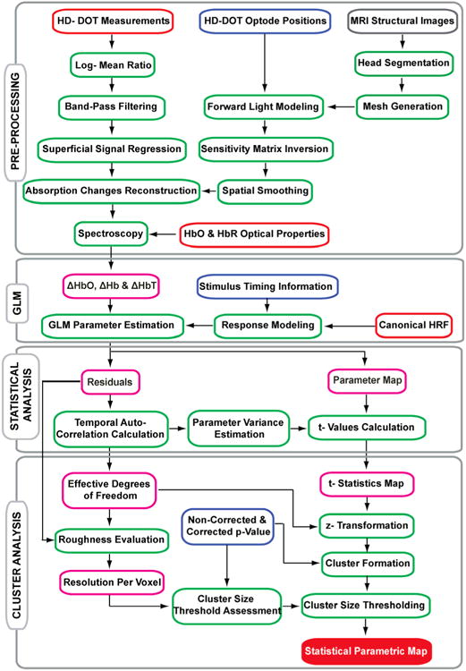
Statistical parametric mapping flowchart. Pre-processing, General linear modeling, Statistical analysis and Cluster analysis.
For visualization of results, we up-sampled the images to 1 mm3. Volumetric activations are overlaid on subject-specific T1 weighted images (with masking skin/scalp and skull). For the cortical surface representation of results all volumetric activation data are mapped onto the subject-specific cortical surface in the Caret 5.65 software package (Van Essen et al., 2001) (http://brainvis.wustl.edu/wiki/index.php/Caret:About).
2.3. General linear model
The general linear model expresses hemodynamic changes at each voxel of the brain as a linear combination of independent variables (i.e. response to different stimuli) and an error term (Friston et al., 1995). Mathematically the GLM is presented by Eq. 1:
| (1) |
The data Y ∈ RT×N are arranged in a matrix that has the dimensions of time (with T elements) and position (a three dimensional space indexed by a single index variable n with N elements). The design matrix X ∈ RT×S has S columns that each represents the modeled response to one of the S different stimuli or conditions. The spatial patterns of responses are embedded in β ∈ RS×N. The error term e ∈ RT×N has the same dimension as the data, and is assumed to be zero-mean Gaussian noise (the assumption of independent errors) with variance matrix Σe = σ2 I (σ2 is variance in the error and I is identity matrix). With these assumptions the method of least squares produces the minumum variance unbiased estimate of the β parameters (Gauss–Markov theorem):
| (2) |
The parameter estimate variance is given by:
| (3) |
In Eq.3, c is the contrast vector which extracts the parameter of interest from β̂, and has the same length as the number of rows of β̂ (e.g. to extract the response to the first condition/stimulus type, c = [1 0], and to extract the response to second condition/stimulus c = [0 1] is used, respectively).
With above assumptions, under the null hypothesis (no activation, H0: ct β̂ = 0), the following statistic,
| (4) |
has a t-distribution with degrees of freedom equal to T – S (Moore and McCabe, 2002).
The design matrix can be constructed by convolving the experimental protocol with a canonical hemodynamic response function (cHRF). cHRF is a standard model for the hemodynamic activity generated in response to an impulse neural activation. In this way, design matrix incorporates a priori knowledge about the timing of stimuli and the hemodynamic response (HDR). We used a two-gamma function (Eq. 5) as our cHRF:
| (5) |
where f(t) is the hemodynamic response t seconds after a stimulus presentation. The first term models the initial signal increase after the stimulus and the second term models the post-stimulus undershoot. For each term, αi determines the amplitude, δi determines delay, ki and τi are two parameters that determine the shape and scale of the curve respectively and Γ(n) = (n − 1)!
The parameters of this function were derived by fitting it to the in vivo data. First, using our traditional block-averaging method, we retrieved the block averaged hemodynamic responses (HDRs) (block averaging was applied to data acquired during block design stimulus) for each subject (here, in addition to our six subjects, we included data from four other subjects which had participated in our previous studies with similar stimulus design). We then fitted the two-gamma function (convolved with a single square wave stimulus) to the average HDRs at a region in the visual cortex with maximum response to visual stimulus (i. e. peak region in the block averaged activation map). Finally, the fitting results were averaged over all subjects and used as parameters for the HD-DOT data-driven cHRF.
2.4. Addressing the temporal autocorrelation issue
In practice the assumption of independent errors (Σe = σ2I) is not met. In addition to some un-modeled physiology, structural noise in the data causes the residuals of GLM to be temporally correlated (Σe = σ2V,where V is the autocorrelation matrix). One of the consequences of this autocorrelation is that Eq. 2 is not the best unbiased estimation of parameters. The other consequence is that the degrees of freedom are decreased to less than the number of samples. In addition, because the structure of noise is not spatially stationary, the degrees of freedom are position dependent.
To deal with the first issue, instead of correcting the β estimate, we corrected the parameter estimate variance (Eq. 3) using information from the statistics for the temporal autocorrelation (Woolrich et al., 2001). The autocorrelation matrix V is assessed for each voxel by evaluating the temporal autocorrelation profile in that voxel's residuals (r = Y − Xβ̂). Details regarding autocorrelation matrix estimation are found in Appendix A. The corrected parameter estimate variance is:
| (6) |
where (X)+ = (XtX)−Xt and σ̂2 is the unbiased estimation of variance σ2 which is given by dividing the sum of squares of the residuals into the expected value for the sum of squares of the standardized residuals (Eq. 7). By standardized we mean normalized so that the variance is one.
| (7) |
R = I − X(XtX)−Xt is the residual forming matrix.
The effective degrees of freedom (for null hypothesis) were estimated using the Satterthwaite approximation, Eq. 8 (Worsley and Friston, 1995):
| (8) |
Details about the Satterthwaite approximation (SA) can be found in Appendix A.
2.5. Addressing the multiple comparison problem
In order to find which regions of the brain show a statistically significant response we need to apply a threshold so that the overall false positive rate in the thresholded map does not exceed the overall false positive rate of interest. There are a variety of solutions to the multiple comparisons problem. Here we used a cluster size analysis based on random field theory (RFT), which is widely used in fMRI (Cao and Worsley, 2001; Friston et al., 1994; Hayasaka and Nichols, 2003; Hayasaka et al., 2004; Worsley et al., 1996). By taking the smoothness (or roughness) of underlying images (random fields) into account, it provides a threshold for the extent of significant foci in a statistical map. This threshold is given by Eq. 9:
| (9) |
where K is the cluster size (in voxel units), p is the overall false positive rate and μ is the expected number of clusters given by RFT (Eq. 10). For more detail please see Appendix B.
| (10) |
Rtotal = N/(FWHM)3, where N is the number of voxels in the image and FWHM is a measure of smoothness of the image in the form of full- width at half maximum (FWHM) of point spread function. Rtotal is called total number of resolution elements (ResEl), it is a concept introduced by (Worsley et al., 1992). zth is the threshold applied to the z-map or Gauassianized t-map (Worsley, 2005) and
| (11) |
where Γ() is mathematical gamma function, and P(Z > zth) is the voxel-level p-value associated with the threshold zth.
Since the point spread function of DOT images is not stationary over the imaging field (resolution depends on location), to calculate the expected number of clusters (μ), we incorporated a non-stationary random field approach in which the local measures of roughness were used to express the resolution per voxel (RPV). RVP can be thought as the ratio of the voxel volume over the volume of the local point spread function, or resolution element (i. e. RPV is a number less than or equal to one, it is one if one voxel is one resolution element). Eq. 12 indicates the relationship between RPV and the local roughness matrix (Λ).
| (12) |
A robust way to estimate the roughness matrix is to calculate the covariance matrix of the spatial partial derivatives of standardized residuals (Kiebel et al., 1999; Worsley et al., 1999). The standardized residual, s, is given by Eq.13.
| (13) |
where r denotes the residual signal (data after subtracting off the GLM). The jkth component of roughness matrix (Λ̂) for voxel ν, λ̂jk(ν), is
| (14) |
where df(ν) is the degrees of freedom for that voxel. ∂S(ν)/∂lj is the spatial derivative of s in direction j. The total number of resolution elements in the whole field (ROI) is
| (15) |
So, substituting Eq. 15, 10 and 11 into Eq. 9 completes the formula for determining the appropriate threshold for a cluster size at given p-value. The cluster size in ResEl units is given by multiplying it by Rtotal/N.
3. Secondary approaches
3.1. Subject specific models
In both fMRI (Aguirre et al., 1998; Handwerker et al., 2004; Miezin et al., 2000) and NIRS (Jasdzewski et al., 2003; Schroeter et al., 2003; Yang et al., 2007) studies, it has been seen that the temporal profile of the HDR varies, in timing, amplitude, and shape from subject to subject, and from region to region within a single subject. Also, the temporal profiles for HbO and HbR are not the same. This means that a cHRF is not the best model for a given HDR since it does not consider these differences. To build a more accurate model for our data, we developed a two-step procedure. From the extracted parametric maps using the canonical GLM, we found a highly responsive voxel for each distinct region (one voxel in the left and one voxel in the right visual cortex) and averaged signals of all voxels inside a cube of 5 by 5 by 5 voxels centered on that voxel. Then using new design matrix, which only incorporated information about the timing of stimuli, we were able to un-mix the HDR to a single stimulus from the overlapping responses to event-related stimuli. By applying this procedure for each region and each contrast for each subject we calculated region-, subject-, and the contrast-specific response models. Finally, we rebuilt the design matrix and extracted the activation maps.
3.2. Temporal autocorrelations
As discussed previously, temporal autocorrelations in the residuals violate the assumption of independent errors made in using the least squares method for parameters' estimation. A number of approaches exist to deal with this issue. One common approach, pre-whitening, removes autocorrelations by applying a pre-whitening matrix, so that the residuals become independent and the assumptions of the least squares method become valid (Bullmore et al., 1996; Friston et al., 2002; Hofmann et al., 2008; Koh et al., 2007; Plichta et al., 2006). A second common method is shaping the structure of autocorrelations by temporally smoothing data (Worsley and Friston, 1995). This method, known as pre-coloring, tries to swamp and negate the effects of not accurately knowing the intrinsic autocorrelations by imposing known autocorrelation. Here we have evaluated and compared the efficiency of those methods with the correction of variance method used in this study. The efficiency of each method is inversely proportional to the variance of the parameter estimates by that method (Woolrich et al., 2001), Eq. 16.
| (16) |
ζ is efficiency. Details regarding the variance estimation for pre-colored and pre-whitened results can be found in Appendix A.
Here we also offer a simple intuitive way for the estimation of effective degrees of freedom and call it the independent sample approximation (ISA). In this approach the FWHM of the temporal autocorrelation function (calculated from residuals, Appendix A) is used as a measure of the extent of dependency between samples. The effective degrees of freedom is given by
| (17) |
Where T is number of samples (the sample rate is 1 Hz) and S is number of regressors (number of columns in the design matrix) (Moore and McCabe, 2002). In principal, either method can be used since both are an approximation, and we evaluate both for completeness.
3.3. Cluster height threshold
In the procedure presented in the previous section, in order to control the false positive rate a threshold for the size of clusters was evaluated. The shortcoming of this approach is that if the cluster height is ignored, then sensitivity to small activation foci is lost. To overcome this issue, we also evaluated a threshold for the cluster height (Friston et al., 1991; Worsley, 1995; Worsley et al., 1992; Worsley et al., 1996) using a non-stationary RF approach and combined these two thresholds. A cluster was classified as significant if its spatial extent was equal to or larger than the cluster size threshold or if its height was equal or larger than the cluster height threshold. To find this cluster we evaluated two different p-values for it: one was pheight, the probability of finding at least one voxel with a statistical value above the height threshold in that cluster by chance (for more details please see Appendix B), and the other was psize, the probability of finding a cluster of that size in whole FOV by chance. If any of these p-values was less than p-value of interest, then that cluster would be known as a region with significant activation
4. Experimental results
4.1. General linear model
Extracted hemodynamic responses from block and event-related data demonstrate that the linear model effectively de-convolves oxy-hemoglobin (HbO) concentration changes during a fast (relative to the HDR function) series of mixed visual stimuli (Fig. 2 (a-f)). Similar results were obtained for deoxy-hemoglobin (HbR) and total hemoglobin (HbT) (Supplementary Figure 1). To localize activation responses with the event related data, we first estimated a canonical hemodynamic response function (cHRF) by fitting the two-gamma function to the block averaged HbO signals at the peak signal region in the individual subjects' block averaged maps (Fig. 2(g)). Averaged parameters (Table 1) were used to define a cHRF and form the design matrix for the GLM. The event-related activation maps, as we expected, represent a localized response in the contralateral side of the visual cortex very similar to block averaged maps (Fig. 2 (h-k)). Similar maps were obtained for deoxy-hemoglobin (HbR) and total hemoglobin (HbT) (Supplementary Figure 1). To evaluate the full statistical parametric mapping, we evaluated the degrees of freedom (Fig. 3), the spatially dependent smoothing (Fig. 4) and the cluster analysis based SPMs (Fig. 5).
Fig. 2.

GLM un-mixing works for rapid event related multi-stimuli design. (a) HbO changes during left and right visual stimulus presentation in a block design for a voxel in the left and a voxel in the right visual cortex (LVC and RVC respectively) of subject 1. Stimulus is on for 5 s and off for 30 s. (b) and (c) are extracted hemodynamic (in these two voxels) using GLM un-mixing of response to the left and right stimuli respectively. (d), (e) and (f) are similar results for the event-related stimulus design, where stimulus is on for 5 s and off for an interval randomly selected from 2 – 15 s. Mean inter stimulus interval is 8.4 s. (g) A modeled hemodynamic response function (HRF). Two-gamma function was fitted to block averaged HbO changes for different subjects. Two gamma function for the averaged values of the parameters over 10 subjects'/sessions' fits (black line) used as canonical HRF. Delay, raising time and decay times are shown. (h) and (i) are activation maps showing the location of activation in response to the left and right stimuli, respectively, presented in the block design. (j) and (k) are activation maps in response to event-related presentation of the left and right stimuli. These are subject 1's HbO responses. Maps are shown in parasagittal, axial, coronal and posterior views. The volumetric activations are overlaid on subjectspecific T1 images and thresholded at 10% of maximum.
Table 1.
Parameters of two-gamma function averaged over 10 subjects and sessions fitting results.
| Parameter | α1 | τ1 | k1 | δ1 | α2 | τ2 | k2 | δ2 |
|---|---|---|---|---|---|---|---|---|
| Mean± Std | 1.3±0.2 | 2.5±0.9 | 3.2±0.8 | 2.6±1.3 | -0.5±0.2 | 3.0±0.8 | 2.2±0.8 | 11.5±2.0 |
Fig. 3.
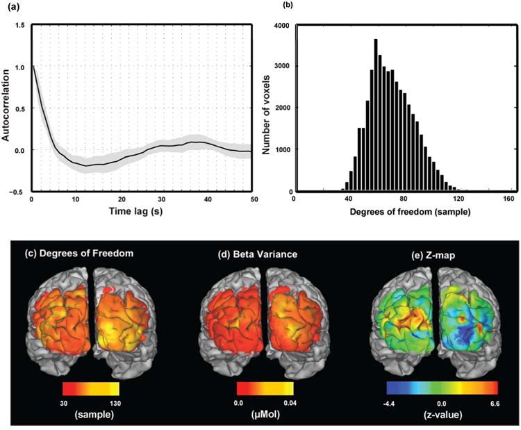
Temporal autocorrelation and degrees of freedom depend on location. (a) Average temporal autocorrelation profile in GLM residuals (averaged over all voxels in ROI). Only the first 50 time lags are shown. (b) Histogram of effective degrees of freedom estimated using Satterthwaite approximation. (c) Map of the effective degrees of freedom. (d) Square root of the variance in the parameter estimates. (e) Map of z-statistics for estimated response to stimulus on the right side of the visual field. These results are for subject 1.
Fig. 4.

Resolution per voxel (RPV) and spatial smoothness are not stationary over ROI. (a) Histogram of resolution per voxel in Voxel-3 units (1 Voxel-3 is 0.125 mm-3). (b) Histogram of geometric mean of full width in half maximum (FWHM) in voxel units (1 voxel is 2 mm). (c) Map of FWHM in posterior surface view. These results are for subject 1.
Fig. 5.

Statistical parametric maps for six subjects: (a-f) SPMs after applying size and height thresholds (see text) for subjects 1-6 respectively.
4.2. Addressing the temporal autocorrelation issue
To assess the effective degrees of freedom (eDOF) in the data and calculate the variance of (GLM) parameter estimates, we evaluated the temporal autocorrelation of the residual signal for each voxel (Fig. 3 (a)) and corresponding autocorrelation matrix. Using these estimates, eDOF and t-statistics maps were generated and transformed to z-statistics maps (Gaussianized t-map) (Fig. 3 (b-e)). Results show that eDOF over whole FOV and for all subjects almost always (> 96%) is above 30 (Supplementary Fig. 2 (a-f)) which meets one of requirements for random field theory (Hayasaka and Nichols, 2003).
4.3. Addressing the multiple comparison problem
To account for the multiple comparison problem, a cluster size threshold was assessed. First the number of resolution elements per voxel (RPV) was evaluated for each data set from residuals of the corresponding GLM fitting (Fig. 4 (a)). The geometric averages of the FWHM of the spatial smoothing curve (= RPV-1/3) were calculated at each voxel (Fig. 4 (b-c)). Results show that the FWHM is not the same everywhere in the FOV however almost all (> 99%) of voxels (in all subjects' data) have FWHM greater than three voxels (Supplementary Fig. 3(a-f)). So, the second requirement of the RFT (smoothness larger than three voxels, (Hayasaka and Nichols, 2003)) is met. Note that the FWHM is distributed around the size of the point spread function for our imaging array which is estimated to be ∼14 mm or 7 voxels (White and Culver, 2010b). We also checked the RPV numbers by summing the RPV values across all voxels in the FOV. The total number of resolution elements, for these six subjects, ranges from 0.2 % to 0.4 % of the total number of voxels in the FOV (which matches the FWHM estimate of 73 ∼ 430 voxels).
To establish the cluster size we set the overall false positive rate p to 0.05and cluster forming threshold zth to 3.09 (corresponding to an uncorrected voxel level p-value of 0.001) and calculated the cluster size threshold (from Eq. 9) and converted it to ResEl units (by multiplying it into the total number of ResEl and dividing into the toltal number of voxels in the FOV). The estimated cluster size threshold for these data ranges from 0.35 to 0.37 ResEls. By applying threshold zth to the Gaussianized t-map (Gt-map), a number of clusters were obtained. The size of each cluster, in ResEl units, was calculated by summing the RPV of all voxels inside that cluster. Clusters with the size equal or larger than the estimated cluster size threshold were defined as significant activation foci in the statistical parametric maps (Fig. 5 (a-f)).
These results conclude the full statistical analysis of the event-related data using the primary processing stream. We also evaluated three alternate approaches previously established in fMRI, including the use of: a) subject specific hemodynamic response models, b) alternate approaches to dealing with the temporal autocorrelation and eDOF estimation, and c) the use of cluster height in addition to the cluster size for setting significance thresholds.
4.5. Subject specific model – Secondary approach
To evaluate the potential optimization of data modeling the subject specific hemodynamic response model was directly extracted from data for each subject (Fig.6 (a)) and incorporated into a subject specific design matrix. The statistical comparison between results of the canonical GLM (cGLM) and the subject specific GLM (ssGLM) indicates a significant (p < 10-5) increase in average z-value (so in the statistical power) for oxy-hemoglobin (Fig. 6 (b)). Similar results were obtained for other hemoglobin contrasts. As with the previous results, the localization of activation using HbO, HbR and HbT are qualitatively similar, however the ssGLM model resulted in higher β (and z-values) (Fig. 7). A paired comparison of statistical power between HbO, HbR and HbT did not show any significant difference (p >0.05) between the three contrasts (Fig. 7 (b)). These comparisons were done by averaging the z-values over all subjects' voxels (inside the significant clusters).
Fig. 6.

Subject specific model increases statistical power. (a) Extracted hemodynamic response (HDR) from different subjects' HbO data acquired during a 5 s event-related stimuli. Canonical HRF convolved with a single trial of stimulus (a 5 s box car function) is shown in black. (b) Comparison of statistical values between canonical model (cGLM) and subject-specific model (ssGLM). These z-values are averaged z-values over all voxels known as significant in the SPMs' of all subjects. Significant difference between two models found at p < 10-5.
Fig. 7.
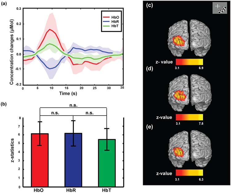
Localization and statistical power of oxy- and deoxy- and total-hemoglobin (HbO, HbR and HbT respectively) are similar. (a) Extracted changes in HbO, HbR and HbT for six subjects, in response to 5 s event-related stimulus, are averaged. (b) Comparison of statistical values between HbO, HbR and HbT shows that there is not a significant difference between statistical values for HbO, HbR and HbT results at p<0.05. These z-values are averaged z-values over all voxels known as significant in the SPMs' of all subjects for each contrast. (c) Activation maps extracted for HbO, HbR and HbT using subject and contrast-specific GLM (ssGLM).
4.6. Temporal autocorrelation – Secondary approach
Since there are several approaches to address the temporal autocorrelation we evaluated them by comparing their efficiency. The comparison (Table 2) showed that the pre-whitening is the most efficient and the correction of variance, is more efficient than the pre-coloring. Since pre-whitening needs very accurate estimation of whitening matrix, otherwise it will introduce bias to the parameter estimate, it needs an iteration to accurately whiten data, and hence increased computation time is required. Considering this, we preferred the correction of variance which needs less computational time and has reasonable efficiency. For the sake of completeness we estimated the eDOF using independent sample approximation (ISA) approach in addition to Satterthwaite approximation. Both approaches appear to give similar results and no clear pattern or significant difference between two methods was detected (Table 3).
Table 2.
A comparison of pre-coloring, variance correction and pre-whitening, applied to HbO data of 6 subjects. The efficiency of pre-coloring and pre-whitening relative to efficiency of variance correction are shown in this table.
| Subject | Pre-Whitening | Pre-Coloring |
|---|---|---|
| 1 | 1.27 | 0.20 |
| 2 | 1.25 | 0.09 |
| 3 | 1.317 | 0.09 |
| 4 | 1.33 | 0.12 |
| 5 | 1.30 | 0.60 |
| 6 | 1.33 | 0.16 |
Table 3.
Effective degree of freedom, estimated by Satterthwaite approximation (SA) method and independent sample approximation (ISA) method. These are results for six subjects and two experimental (Block and Event) protocols. These numbers are averaged over all voxels in the FOV. The number of samples was 381 and 404 for Block and Event protocol respectively.
| Subject | Method | Block | Event |
|---|---|---|---|
| 1 | ISA | 57 | 71 |
| SA | 50 | 70 | |
|
| |||
| 2 | ISA | 74 | 81 |
| SA | 90 | 97 | |
|
| |||
| 3 | ISA | 66 | 75 |
| SA | 73 | 78 | |
|
| |||
| 4 | ISA | 62 | 75 |
| SA | 62 | 70 | |
|
| |||
| 5 | ISA | 75 | 81 |
| SA | 91 | 93 | |
|
| |||
| 6 | ISA | 56 | 81 |
| SA | 48 | 66 | |
4.7. Cluster height threshold – Secondary approach
To facilitate locating small foci with significant activation strength, we also considered the magnitude, or height of each cluster. We applied threshold at zth = 3.09 (corresponding to uncorredted voxel level p-value of 0.001). For all clusters we evaluated the corresponding false positive rate for the height and extent (size), pheight and psize. If one or both of them were less than the p-value of interest (set to 0.05), the cluster was classified as significant. As expected, by adding in an optional test of significance, this procedure captures and defines more clusters as significant (Table 4).
Table 4.
This table contains information about the clusters in the statistical maps of six subjects. The total number of clusters above threshold zth = 3.09 (corresponding with voxel level p-value (non-corrected p-value) of 0.001) on the left and right visual cortex, the height (amplitude) and size (extent) of each cluster are shown. Cluster size is in ResEl units. The pheight and psize (as defined in the text) are also included.
| Subject | Total number of clusters | Cluster's Height (z-value) | Cluster's Size (ResEls) | pheight | psize |
|---|---|---|---|---|---|
| 1 | Left : 2 | 4.8933* | 1.5353 | 0.0007 | 0.0064 |
| 3.1264 | 0.0249 | 0.3240 | 0.7234 | ||
|
| |||||
| Right: 3 | 5.6580* | 3.3949 | 0.0000 | 0.0002 | |
| 3.0906 | 0.0002 | 0.3530 | 0.9864 | ||
| 3.4339 | 0.0545 | 0.1454 | 0.5796 | ||
|
| |||||
| 2 | Left : 2 | 6.0323* | 6.5460 | 0.0000 | 0.0000 |
| 4.2157* | 0.3230 | 0.0136 | 0.1346 | ||
|
| |||||
| Right: 1 | 5.5483* | 2.1155 | 3.6235e-05 | 8.9350e-04 | |
|
| |||||
| 3 | Left : 1 | 4.9198* | 1.9672 | 6.7708e-04 | 0.0018 |
| 4.6893* | 2.4688 | 0.0019 | 0.0006 | ||
|
| |||||
| Right: 3 | 3.6118 | 0.0729 | 0.0932 | 0.4945 | |
| 4.7991* | 0.8882 | 0.0012 | 0.0240 | ||
|
| |||||
| 4 | Left : 1 | 5.5429* | 3.3056 | 3.0654e-05 | 2.3089e-04 |
|
| |||||
| Right: 2 | 4.6239* | 0.8469 | 0.0022 | 0.0341 | |
| 3.8269* | 0.0902 | 0.0436 | 0.4682 | ||
|
| |||||
| 5 | Left : 2 | 4.1475* | 0.6069 | 0.0075 | 0.1404 |
| 3.3215 | 0.2013 | 0.1016 | 0.3903 | ||
|
| |||||
| Right: 1 | 5.4230* | 1.5197 | 3.0000e-5 | 0.0217 | |
|
| |||||
| 6 | Left : 2 | 3.7393 * | 0.4460 | 0.0777 | 0.1229 |
| 3.1181 | 0.0635 | 0.4389 | 0.5646 | ||
|
| |||||
| Right: 1 | 4.1187* | 0.6245 | 0.0215 | 0.0725 | |
Means the cluster is known as significant.
5. Discussion
This paper demonstrates a comprehensive set of statistical tools for analysis of HD-DOT data. Considering temporal and spatial characteristics of HD-DOT signals, we have extended fundamental elements of the statistical parametric mapping of fMRI for HD-DOT. Although previous NIRS studies have addressed these topics in NIRS measurement space, this paper uniquely focuses on the analysis in HD-DOT image space, utilizing the relatively higher image quality afforded by High-Density DOT imaging arrays.
In order to use a rapid event related design with a general linear model to generate activation maps, a priori knowledge about the hemodynamic response function (HRF) is needed. Previous work with NIRS (Zhang et al., 2005) has mixed temporal, spatial, and spectral a priori knowledge about data into a single design matrix, to extract temporal profiles of oxy- and deoxy-hemoglobin changes directly from simulated source-detector measurements, though block averaging has often been used to generate activation maps. In most NIRS's GLM works (Abdelnour and Huppert, 2009; Ciftci, et al., 2008; Cohen-Adad, et al., 2007; Plichta, et al., 2007; Plichta, et al., 2006; Ye, et al., 2009) this prior knowledge is borrowed from the fMRI literature (Glover, 1999; Woolrich et al., 2004). It has usually been either a Gaussian function or a two-gamma function with the BOLD signal's shape and timing characteristics. Although fMRI signal and NIRS signals are correlated (Cui et al., 2011; Huppert et al., 2006; Mehagnoul-Schipper et al., 2002; Sassaroli et al., 2006; Strangman et al., 2002; Toronov et al., 2001), there is still enough deviation in their temporal profile to suggest that a response model specific to NIRS/DOT data can provide better statistical power in detection and localization of brain response. Therefore assuming a generic form of a two-gamma function for HDR, we found that following a brief (duration ≪ 1s) visual stimulation, HbO signal changes start with 2-3 s delay and raises to its peak in approximately 6 s (time to peak from the start of stimulus was ∼ 8 s), with an undershoot that happens at around 18 s. The approximate FWHM was found to be 7.5 s for first peak and ∼ 8 s for the undershoot. These numbers are different from the numbers mentioned in fMRI literature for several potential reasons (see (Savoy et al., 1994) (Glover, 1999) and the cHRF used in SPM software package (Wellcome Trust Centre for Neuroimaging, London, UK), and the supplementary table). In addition to differences in the physiology and measurement physics of the BOLD and HbO signals, these differences are also likely due to a number of differences in protocol (e.g. stimuli duration) and signal processing (e.g. temporal filtering).
By incorporating the obtained cHRF in linear modeling of event-related data, we confirmed that HD-DOT is capable of de-convolving overlapping responses and producing localized brain responses for two inter-mixed stimuli (Fig. 2). This important test of rapid event-related functional imaging demonstrates that un-mixing of two different stimuli with overlapping hemodynamic responses is possible. It tailors access to more flexible paradigms that model neuronal events associated with real cognitive processes (D'Esposito et al., 1999) and reduces potential confounds due to strategy effects, prediction and habituation (Dale, 1999; Rosen et al., 1998).
A comparison of the different hemoglobin contrasts shows that the activation patterns are very similar (Supplementary Figure 1) while the amplitude of the spatial response is higher for HbO compared to two others. The stronger HbO response results from a larger change in the oxygenated hemoglobin concentration and possibly due to a better fitting of the model to the HbO data since the cHRF was built based on the HbO data. These ambiguities in addition to differences in the individual's brain response that has been reported in previous fMRI (Aguirre et al., 1998; Handwerker et al., 2004; Miezin et al., 2000) and NIRS literatures (Jasdzewski et al., 2003; Schroeter et al., 2003; Yang et al., 2007), necessitates additional work to optimize the model. A common way to overcome this issue has been using the first and sometimes first and second derivatives of the cHRF in the design matrix. Although using this approach they were able to accommodate variabilities, the main weakness of this approach is that it introduces further complexity into the interpretation and statistical inference about obtained results. We incorporated a method that can help us better model the data, and provides a more straightforward interpretation of the activation maps, and subsequently the SPMs. By implementing prior knowledge about the stimulus timing in a linear model, we extract the temporal profile of HDR for each contrast, each region, and each subject. We limit this estimation to a set of voxels that were highly responsive to the external stimulus in activation maps resulted from the canonical GLM. So a subject- and contrast specific HDR in each functionally distinct region (left and right visual cortex) were estimated. This approach yielded a similar statistical power for different contrasts and more importantly it caused an improvement in the statistical power in respect to the canonical model (Fig. 6 and Fig. 7). However, a voxel-wise response model or another way to take the differences in the response of different voxels is not addressed in this work.
While most fMRI-SPM and NIRS-SPM (Ye et al., 2009) approaches address the temporal dependency of the residuals, heterogeneity of the temporal autocorrelations is rarely addressed. However it is known that the error variance structure is not the same at all voxels (Friston et al., 2006). Herein we have considered this spatial non-uniformity of noise structure and have evaluated spatially specific measures of the residual signal autocorrelation function and variance-covariance matrix. To correctly calculate statistical t- values we considered three alternative approaches: variance correction, pre-whitening and pre-colouring, and picked the first one for the following reasons. Comparing efficiency, the correction of variance (primary approach) is more efficient than pre-coloring, but is not remarkably less efficient compared to pre-whitening (Table 2). In addition, correction of variance is computationally faster. In addition the correction of variance avoids the potential bias to the GLM solution that might occur with pre-whitening due to potential errors in the pre- whitening matrix. To determine effective degrees of freedom (eDOF), in addition to using Satterthwaite approximation, which is commonly used in previous works, we introduced a simple and intuitive method of independent sample approximation. eDOF in the entire FOV for all subjects estimated with these two methods although were not exactly same they were relatively high (> 96 % eDOF was above 30). Having eDOF at each voxel we transformed t-maps to z-maps.
The next step was defining confidence thresholds for specified p-values across the images. To do so, we must address the multiple comparisons problem in order to control the false positive rate. There are numerous approaches to this issue (Nichols and Hayasaka, 2003), here we demonstrated the use of RFT. While permutation and RFT provide thresholds for both height and spatial extent of the significant activation, Bonferroni correction adjusts the height threshold by decreasing the per voxel false positive rate proportionally to the number of voxels. However, HD-DOT data are spatially correlated (smooth) mainly due to smooth physiological signal (collective response of neighboring neurons, and expanded vascular response) and a limited resolution (point spread function). While RFT explicitly takes into account this spatial smoothness and provides a formula for the estimation of thresholds (Friston et al., 1994; Petersson et al., 1999; Worsley et al., 1992; Worsley et al., 1996), the Bonferroni correction ignores this and assumes data are spatially independent, and becomes overly conservative in these conditions. RFT is valid under specific assumptions: sufficient smoothness, sufficiently high threshold, and stationary smoothness all over the imaging field (Petersson et al., 1999; Worsley et al., 1992; Worsley et al., 1996). An evaluation of this method (Hayasaka and Nichols, 2003) with simulation of data under a varying smoothness, threshold and degree of freedom showed that it is valid for degrees of freedom higher than 30 and FWHM of smoothness larger than 3 voxels. Although the stationary assumption does not exist for our data (Fig. 4), the degrees of freedom (Fig. 3(b)) and smoothness (Fig. 4) meet required conditions. Quantitatively speaking the effective degrees of freedom in most of voxels (>96%) in the FOV for all subjects found to be above 30 (from ∼ 404 samples). From table 3, mean of degrees of freedom of all subjects' is 87. Roughly speaking to have at least 30 degrees of freedom we need around 150 samples (30*(404/87)∼150). Also our results show that above 99% of voxels in the FOV have FWHM of higher than 3 voxels. Accordingly, to take the non-uniformity of smoothness into account we implemented a non-stationary cluster analysis based on RFT (Hayasaka et al., 2004; Worsley, 2002; Worsley et al., 1999). We estimated roughness at each voxel and the contribution of each voxel in the total number of resolution elements in terms of resolution per voxel (RPV). Generally borders of ROI are the roughest areas (maximum RPV for 6 subjects in this study ranged from 0.004 to 0.008) and roughness deceases with depth (minimum RPV ranged from 10-5 to 10-4) and the mean value was 0.0028. These numbers are more intuitive if we convert them to the FWHM of the point spread function (FWHM =2×RPV-1/3 mm), where the mean RPV converts to mean FWHM of 14 mm. Our results are in agreement with (White and Culver, 2010b) who reported the resolution of similar imaging array to be 14 mm and (Zhan Y, 2012) who showed the resolution decreases with depth. The extent (size) of the clusters in the statistical maps thresholded at primary height threshold of 3.09 was compared with the estimated size thresholds to determine the significance of the cluster. In order to optimize the detection power we also considered the height of the cluster. So, a cluster was labeled as significant if either its size was larger than size threshold or its height passed the height threshold. This procedure resulted in detection of at least one significant activation foci per stimulus type for all subjects (Table 4). However, if the Bonferroni correction was used no significant activations were found in subject 6 or for the right stimulus in subject 5. Quantitatively, the voxel – level height threshold given by Bonferroni correction for these six subjects ranged from 4.17-4.45 which exceeds the threshold used in the RFT approach and the maximum z- value in the SPMs of subject 5 and 6 (Fig.5 (e) and (f)).
Future extensions of this research may continue to optimize aspects of the modeling. For instance, the noise structure in GLM residuals could be modeled explicitly in the design matrix. So, instead of applying temporal high and low pass filters on raw data in measurement space (source-detector pair measurements) to remove low frequency drifts (e.g. respiration and cardiac pulsations), the noise sources could be included as regressors in the GLM to explicitly model these nuisance signals. Since RFT has some limitations (assumptions), a more general way to address the multiple-comparison problem is desired. For instance the permutation test is known to perform well under any setting such as low degrees of freedom and low smoothness (Hayasaka et al., 2004; Nichols and Holmes, 2002; Smith and Nichols, 2009; Worsley, 1977) and can be used to build the probability distribution of cluster height and size (under null hypothesis) from data. However permutation based approaches are computationally intensive.
6. Conclusion
We have demonstrated how HD-DOT data can be accurately and efficiently analyzed within a comprehensive GLM-SPM framework comparable to that widely-used for fMRI data. Most importantly, this includes the use of event-related designs and principled control for false positives. These advances facilitate the adoption of more complex event-related experimental paradigms and a more rigorous treatment of the results, paving the way for future advancement of HD-DOT.
Supplementary Material
Supplementary Fig. 1: Similar results are obtained for deoxy- and total- hemoglobin (HbR and HbT respectively) changes during rapid event related visual stimulation (a) HbR changes during left and right visual stimulus presentation for a voxel in the left and a voxel in the right visual cortex (LVC and RVC respectively) of subject 1. (b) and (c) are extracted hemodynamic (in these two voxels) using GLM un-mixing of response to the left and right stimuli respectively. (d) and (e) are activation maps showing the location of activation in response to the left and right stimuli, respectively. (f-j) are similar results for HbT data.
Supplementary Fig. 2: (a-f) Histogram of effective degrees of freedom for subjects 1-6 respectively.
Supplementary Fig. 3: (a-f) Histogram of FWHM for subjects 1-6 respectively.
Acknowledgments
We thank Gavin Perry and Martin Olevitch for help with HD-DOT instrumentation and software and Jonathan Peelle for critical reading and review. This work was supported in part by NIH grants R01-EB009233 (J.P.C), R01-NS078223 (J.P.C.), Autism Speaks Postdoctoral Translational Research Fellowship 7962 (A.T.E.), and a Fulbright Science and Technology Ph.D. Award (S.L.F.). The funding source had no involvement in the study design, collection, analysis, interpretation of the data, writing of the paper, or decision to submit the paper for publication. J.P.C and Washington University have financial interests in Cephalogics LLC based on a license of related optical imaging technology by the University to Cephalogics LLC.
Appendix A
Autocorrelation matrix estimation
For given voxel j the temporal autocorrelation at time lag of m is given by
| (A.1) |
is the residual at voxel j at timepoint i and is the mean of residuals at that voxel.
The covariance matrix V would be
| (A.2) |
Satterthwaite approximation
In Satterthwaite approximation we assume sum of squares of residuals (rtr) follows χ2-distribution with scaled χ2-variant (ax)
| (A.3) |
where p(x)∼χ2(df), df is effective degrees of freedom. For χ2(df) distribution we have, E{x} = df and Var{x} = 2df (E{.} is expectation operator and Var{.} is variance operator). So,
| (A.4) |
| (A.5) |
So,
| (A.6) |
Note that r = RY and R = I − X(XtX)−Xt and it is easy to show that R = Rt = RtR and Var{Y} = Var{e} = σ2V.
| (A.7) |
Basic properties of trace operator is used such as trace(AtB) = trace(BtA) and trace(ABCD) = trace(BCDA) = trace (CDAB) = trace(DABC).
In the similar way one can show
| (A.8) |
So, the effective degree of freedom is
| (A.9) |
Pre-coloring and Pre-whitening
One of approaches to deal temporal autocorrelation issue in parameter estimation is pre-coloring which substitutes unknown autocorrelation with a known autocorrelation. Data are temporally smoothed with a known smoothing kernel that matches the hemodynamic response function (Friston et al., 1995; Worsley and Friston, 1995). The variance of the parameter estimates would be
| (A.10) |
where G is smoothing kernel.
Other method is pre-whitening (Bullmore et al., 1996) which estimates the autocorrelation structure and removes it from data. The variance of parameter would be
| (A.11) |
where V = KKt is the covariance matrix and K− is pre-whitening matrix.
Efficiency (ζ) of these methods can be evaluated using Eq. A.12 (Woolrich et al., 2001).
| (A.12) |
Appendix B
Random field theory
Random field theory is a branch of mathematics that is used in solving the multiple comparison problem in neuroimaging, because a z-map (or a Gaussianized t-map, Gt-map) can be considered as a Gaussian random field. RFT depends on the statistic of a quantity called Euler characteristic (EC). EC can be roughly defined as number of peaks (blobs) minus number of valleys (holes) that are above a given threshold in a continuous Gaussian field (Ashby, 2011).
Since at high thresholds the number of clusters (blobs), m, and Euler characteristic (EC) converge, the probability of having one cluster or more, P(m ≥ 1), is approximately equal to probability of EC ≥ 1, (P(EC ≥ 1)). In addition, at high thresholds EC is either one or zero, so, the expected value of EC is equal to the probability of EC ≥ 1. So, at high thresholds
| (B.1) |
The probability finding at least one cluster of size at least one voxel, P(m ≥ 1) under null situation is same as the probability of one false positive. Thus, the probability of interest is approximately equal to the E{EC}. For D dimensional random field with number of resolution elements of Rtotal, at threshold zth, E{EC} is given by Eq. B.2, (Worsley et al., 1996).
| (B.2) |
Eq. B.2 is used for evaluation of pheight.
Cluster size threshold
For a Gaussian random field the number of clusters follows a Poisson distribution (Adler, 1981). Using this knowledge and assuming the clusters are independent the relation between the overal false positive (p) and the probability of one false positive in a cluster (pc) can be driven (Eq. B.3) (Ashby, 2011).
| (B.3) |
Where μ is the mean number of clusters. As it was mentioned before at high thresholds EC and number of clusters converge, so, μ = E{m} = E{EC}.
Assuming the null hypothesis to be true in every voxel, at a reasonably high threshold, the probability of a false positive at any cluster with size of larger than K (voxels) is given by Eq.B. 4, (Friston et al., 1994).
| (B.4) |
Where n stands for the number of voxels in that cluster, and
| (B.5) |
Where P(Z > zth) is probability of z-value to be higher than threshold zth under null hypothesis and N is number of voxels in ROI.
Eq. B.4 is used for evaluation of psize.
References
- Abdelnour AF, Huppert T. Real-time imaging of human brain function by near-infrared spectroscopy using an adaptive general linear model. Neuroimage. 2009;46:133–143. doi: 10.1016/j.neuroimage.2009.01.033. [DOI] [PMC free article] [PubMed] [Google Scholar]
- Adler RJ. The Geometry of Random Fields. Wiley; New York: 1981. [Google Scholar]
- Aguirre GK, Zarahn E, D'Esposito M. The variability of human, BOLD hemodynamic responses. Neuroimage. 1998;8:360–369. doi: 10.1006/nimg.1998.0369. [DOI] [PubMed] [Google Scholar]
- Ashby FG. Statistical Analysis of fMRI Data. The MIT Press, Massachusetts Institute of Technology; 2011. p. 352. [Google Scholar]
- Bandettini PA, Jesmanowicz A, Wong EC, Hyde JS. Processing strategies for time-course data sets in functional MRI of the human brain. Magn Reson Med. 1993;30:161–173. doi: 10.1002/mrm.1910300204. [DOI] [PubMed] [Google Scholar]
- Blamire AM, Ogawa S, Ugurbil K, Rothman D, McCarthy G, Ellermann JM, Hyder F, Rattner Z, Shulman RG. Dynamic mapping of the human visual cortex by high-speed magnetic resonance imaging. Proc Natl Acad Sci U S A. 1992;89:11069–11073. doi: 10.1073/pnas.89.22.11069. [DOI] [PMC free article] [PubMed] [Google Scholar]
- Bluestone AY, Abdoulaev G, Schmitz CH, Barbour RL, Hielscher AH. Three-dimensional optical tomography of hemodynamics in the human head. Opt Express. 2001;9:272–286. doi: 10.1364/oe.9.000272. [DOI] [PubMed] [Google Scholar]
- Boas DA, Chen K, Grebert D, Franceschini MA. Improving the diffuse optical imaging spatial resolution of the cerebral hemodynamic response to brain activation in humans. Optics Letters. 2004a;29:1506–1508. doi: 10.1364/ol.29.001506. [DOI] [PubMed] [Google Scholar]
- Boas DA, Dale AM. Simulation study of magnetic resonance imaging-guided cortically constrained diffuse optical tomography of human brain function. Applied Optics. 2005;44:1957–1968. doi: 10.1364/ao.44.001957. [DOI] [PubMed] [Google Scholar]
- Boas DA, Dale AM, Franceschini MA. Diffuse optical imaging of brain activation: approaches to optimizing image sensitivity, resolution, and accuracy. Neuroimage. 2004b;23:S275–S288. doi: 10.1016/j.neuroimage.2004.07.011. [DOI] [PubMed] [Google Scholar]
- Bullmore E, Brammer M, Williams SCR, Rabehesketh S, Janot N, David A, Mellers J, Howard R, Sham P. Statistical methods of estimation and inference for functional MR image analysis. Magnetic Resonance in Medicine. 1996;35:261–277. doi: 10.1002/mrm.1910350219. [DOI] [PubMed] [Google Scholar]
- Cao J, Worsley KJ. Applications of random fields in human brain mapping. In: Moore M, editor. Spatial Statistics: Methodological Aspects and Applications, Springer Lecture Notes in Statistics. Vol. 159. Springer; New York: 2001. pp. 169–182. [Google Scholar]
- Ciftci K, Sankur B, Kahya YP, Akin A. Constraining the general linear model for sensible hemodynamic response function waveforms. Med Biol Eng Comput. 2008;46:779–787. doi: 10.1007/s11517-008-0347-6. [DOI] [PubMed] [Google Scholar]
- Clark VP, Parasuraman R, Keil K, Kulansky R, Fannon S, Maisog JM, Ungerleider LG, Haxby JV. Selective attention to face identity and color studied with fMRI. Human Brain Mapping. 1997;5:293–297. doi: 10.1002/(SICI)1097-0193(1997)5:4<293::AID-HBM15>3.0.CO;2-F. [DOI] [PubMed] [Google Scholar]
- Cohen-Adad J, Chapuisat S, Doyon J, Rossignol S, Lina JM, Benali H, Lesage F. Activation detection in diffuse optical imaging by means of the general linear model. Med Image Anal. 2007;11:616–629. doi: 10.1016/j.media.2007.06.002. [DOI] [PubMed] [Google Scholar]
- Cui X, Bray S, Bryant DM, Glover GH, Reiss AL. A quantitative comparison of NIRS and fMRI across multiple cognitive tasks. Neuroimage. 2011;54:2808–2821. doi: 10.1016/j.neuroimage.2010.10.069. [DOI] [PMC free article] [PubMed] [Google Scholar]
- Custo A, Boas DA, Tsuzuki D, Dan I, Mesquita R, Fischl B, Grimson WEL, Wells W. Anatomical atlas-guided diffuse optical tomography of brain activation. Neuroimage. 2010;49:561–567. doi: 10.1016/j.neuroimage.2009.07.033. [DOI] [PMC free article] [PubMed] [Google Scholar]
- D'Esposito M, Zarahn E, Aguirre GK. Event-related functional MRI: Implications for cognitive psychology. Psychological Bulletin. 1999;125:155–164. doi: 10.1037/0033-2909.125.1.155. [DOI] [PubMed] [Google Scholar]
- Dale AM. Optimal experimental design for event-related fMRI. Human Brain Mapping. 1999;8:109–114. doi: 10.1002/(SICI)1097-0193(1999)8:2/3<109::AID-HBM7>3.0.CO;2-W. [DOI] [PMC free article] [PubMed] [Google Scholar]
- Dale AM, Buckner RL. Selective averaging of rapidly presented individual trials using fMRI. Human Brain Mapping. 1997;5:329–340. doi: 10.1002/(SICI)1097-0193(1997)5:5<329::AID-HBM1>3.0.CO;2-5. [DOI] [PubMed] [Google Scholar]
- Eggebrecht AT, White BR, Ferradal SL, Chen C, Zhan Y, Snyder AZ, Dehghani H, Culver JP. A quantitative spatial comparison of high-density diffuse optical tomography and fMRI cortical mapping. Neuroimage. 2012 doi: 10.1016/j.neuroimage.2012.01.124. [DOI] [PMC free article] [PubMed] [Google Scholar]
- Fransson P, Kruger G, Merboldt KD, Frahm J. Temporal and spatial MRI responses to subsecond visual activation. Magn Reson Imaging. 1999;17:1–7. doi: 10.1016/s0730-725x(98)00163-5. [DOI] [PubMed] [Google Scholar]
- Friston KJ, Ashburner J, Kiebel S, Nichols T, Penny W. Statistical Parametric Mapping: The Analysis of Functional Brain Images. Academic Press; Sandiego, CA, USA: 2006. [Google Scholar]
- Friston KJ, Fletcher P, Josephs O, Holmes A, Rugg MD, Turner R. Event-related fMRI: characterizing differential responses. Neuroimage. 1998;7:30–40. doi: 10.1006/nimg.1997.0306. [DOI] [PubMed] [Google Scholar]
- Friston KJ, Frith CD, Liddle PF, Frackowiak RS. Comparing functional (PET) images: the assessment of significant change. J Cereb Blood Flow Metab. 1991;11:690–699. doi: 10.1038/jcbfm.1991.122. [DOI] [PubMed] [Google Scholar]
- Friston KJ, Holmes AP, Poline JB, Grasby PJ, Williams SC, Frackowiak RS, Turner R. Analysis of fMRI time-series revisited. Neuroimage. 1995;2:45–53. doi: 10.1006/nimg.1995.1007. [DOI] [PubMed] [Google Scholar]
- Friston KJ, Penny W, Phillips C, Kiebel S, Hinton G, Ashburner J. Classical and Bayesian inference in neuroimaging: theory. Neuroimage. 2002;16:465–483. doi: 10.1006/nimg.2002.1090. [DOI] [PubMed] [Google Scholar]
- Friston KJ, Worsley KJ, Frackowiak RSJ, Mazziotta JC, Evans AC. Assessing the significance of focal activations using their spatial extent. Human Brain Mapping. 1994;1:210–220. doi: 10.1002/hbm.460010306. [DOI] [PubMed] [Google Scholar]
- Gibson AP, Austin T, Everdell NL, Schweiger M, Arridge SR, Meek JH, Wyatt JS, Delpy DT, Hebden JC. Three-dimensional whole-head optical passive motor evoked responses in the tomography of neonate. Neuroimage. 2006;30:521–528. doi: 10.1016/j.neuroimage.2005.08.059. [DOI] [PubMed] [Google Scholar]
- Gibson AP, Hebden JC, Arridge SR. Recent advances in diffuse optical imaging. Phys Med Biol. 2005;50:R1–R43. doi: 10.1088/0031-9155/50/4/r01. [DOI] [PubMed] [Google Scholar]
- Glover GH. Deconvolution of impulse response in event-related BOLD fMRI. Neuroimage. 1999;9:416–429. doi: 10.1006/nimg.1998.0419. [DOI] [PubMed] [Google Scholar]
- Habermehl C, Holtze S, Steinbrink J, Koch SP, Obrig H, Mehnert J, Schmitz CH. Somatosensory activation of two fingers can be discriminated with ultrahigh-density diffuse optical tomography. Neuroimage. 2012;59:3201–3211. doi: 10.1016/j.neuroimage.2011.11.062. [DOI] [PMC free article] [PubMed] [Google Scholar]
- Handwerker DA, Ollinger JM, D'Esposito M. Variation of BOLD hemodynamic responses across subjects and brain regions and their effects on statistical analyses. Neuroimage. 2004;21:1639–1651. doi: 10.1016/j.neuroimage.2003.11.029. [DOI] [PubMed] [Google Scholar]
- Hayasaka S, Nichols TE. Validating cluster size inference: random field and permutation methods. Neuroimage. 2003;20:2343–2356. doi: 10.1016/j.neuroimage.2003.08.003. [DOI] [PubMed] [Google Scholar]
- Hayasaka S, Phan KL, Liberzon I, Worsley KJ, Nichols TE. Nonstationary cluster-size inference with random field and permutation methods. Neuroimage. 2004;22:676–687. doi: 10.1016/j.neuroimage.2004.01.041. [DOI] [PubMed] [Google Scholar]
- Heiskala J, Pollari M, Metsaranta M, Grant PE, Nissila I. Probabilistic atlas can improve reconstruction from optical imaging of the neonatal brain. Opt Express. 2009;17:14977–14992. doi: 10.1364/oe.17.014977. [DOI] [PubMed] [Google Scholar]
- Hofmann MJ, Herrmann MJ, Dan I, Obrig H, Conrad M, Kuchinke L, Jacobs AM, Fallgatter AJ. Differential activation of frontal and parietal regions during visual word recognition: An optical topography study. Neuroimage. 2008;40:1340–1349. doi: 10.1016/j.neuroimage.2007.12.037. [DOI] [PubMed] [Google Scholar]
- Hu XS, Hong KS, Ge SS, Jeong MY. Kalman estimator- and general linear model-based on-line brain activation mapping by near-infrared spectroscopy. Biomedical engineering online. 2010;9:82. doi: 10.1186/1475-925X-9-82. [DOI] [PMC free article] [PubMed] [Google Scholar]
- Huppert TJ, Hoge RD, Diamond SG, Franceschini MA, Boas DA. A temporal comparison of BOLD, ASL, and NIRS hemodynamic responses to motor stimuli in adult humans. Neuroimage. 2006;29:368–382. doi: 10.1016/j.neuroimage.2005.08.065. [DOI] [PMC free article] [PubMed] [Google Scholar]
- Jasdzewski G, Strangman G, Wagner J, Kwong KK, Poldrack RA, Boas DA. Differences in the hemodynamic response to event-related motor and visual paradigms as measured by near-infrared spectroscopy. Neuroimage. 2003;20:479–488. doi: 10.1016/s1053-8119(03)00311-2. [DOI] [PubMed] [Google Scholar]
- Joseph DK, Huppert TJ, Franceschini MA, Boas DA. Diffuse optical tomography system to image brain activation with improved spatial resolution and validation with functional magnetic resonance imaging. Applied Optics. 2006;45:8142–8151. doi: 10.1364/ao.45.008142. [DOI] [PubMed] [Google Scholar]
- Josephs O, Turner R, Friston K. Event-related fMRI. Human Brain Mapping. 1997;5:243–248. doi: 10.1002/(SICI)1097-0193(1997)5:4<243::AID-HBM7>3.0.CO;2-3. [DOI] [PubMed] [Google Scholar]
- Kiebel SJ, Poline JB, Friston KJ, Holmes AP, Worsley KJ. Robust smoothness estimation in statistical parametric maps using standardized residuals from the general linear model. Neuroimage. 1999;10:756–766. doi: 10.1006/nimg.1999.0508. [DOI] [PubMed] [Google Scholar]
- Koch SP, Habermehl C, Mehnert J, Schmitz CH, Holtze S, Villringer A, Steinbrink J, Obrig H. High-resolution optical functional mapping of the human somatosensory cortex. Front Neuroenergetics. 2010;2:12. doi: 10.3389/fnene.2010.00012. [DOI] [PMC free article] [PubMed] [Google Scholar]
- Koh PH, Glaser DE, Flandin G, Kiebel S, Butterworth B, Maki A, Delpy DT, Elwell CE. Functional optical signal analysis: a software tool for near-infrared spectroscopy data processing incorporating statistical parametric mapping. J Biomed Opt. 2007;12:064010. doi: 10.1117/1.2804092. [DOI] [PubMed] [Google Scholar]
- Mehagnoul-Schipper DJ, van der Kallen BFW, Colier WNJM, van der Sluijs MC, van Erning LJTO, Thijssen HOM, Oeseburg B, Hoefnagels WHL, Jansen RWMM. Simultaneous measurements of cerebral oxygenation changes during brain activation by near-infrared spectroscopy and functional magnetic resonance imaging in healthy young and elderly subjects. Human Brain Mapping. 2002;16:14–23. doi: 10.1002/hbm.10026. [DOI] [PMC free article] [PubMed] [Google Scholar]
- Miezin FM, Maccotta L, Ollinger JM, Petersen SE, Buckner RL. Characterizing the hemodynamic response: Effects of presentation rate, sampling procedure, and the possibility of ordering brain activity based on relative timing. Neuroimage. 2000;11:735–759. doi: 10.1006/nimg.2000.0568. [DOI] [PubMed] [Google Scholar]
- Moore DS, McCabe GP. Introduction to the Practice of Statistics. W H Freeman & Co; 2002. [Google Scholar]
- Nichols T, Hayasaka S. Controlling the familywise error rate in functional neuroimaging: a comparative review. Statistical Methods in Medical Research. 2003;12:419–446. doi: 10.1191/0962280203sm341ra. [DOI] [PubMed] [Google Scholar]
- Nichols TE, Holmes AP. Nonparametric permutation tests for functional neuroimaging: A primer with examples. Human Brain Mapping. 2002;15:1–25. doi: 10.1002/hbm.1058. [DOI] [PMC free article] [PubMed] [Google Scholar]
- Petersson KM, Nichols TE, Poline JB, Holmes AP. Statistical limitations in functional neuroimaging II. Signal detection and statistical inference. Philosophical Transactions of the Royal Society B-Biological Sciences. 1999;354:1261–1281. doi: 10.1098/rstb.1999.0478. [DOI] [PMC free article] [PubMed] [Google Scholar]
- Plichta MM, Heinzel S, Ehlis AC, Pauli P, Fallgatter AJ. Model-based analysis of rapid event-related functional near-infrared spectroscopy (NIRS) data: a parametric validation study. Neuroimage. 2007;35:625–634. doi: 10.1016/j.neuroimage.2006.11.028. [DOI] [PubMed] [Google Scholar]
- Plichta MM, Herrmann MJ, Baehne CG, Ehlis AC, Richter MM, Pauli P, Fallgatter AJ. Event-related functional near-infrared spectroscopy (fNIRS): are the measurements reliable? Neuroimage. 2006;31:116–124. doi: 10.1016/j.neuroimage.2005.12.008. [DOI] [PubMed] [Google Scholar]
- Rosen BR, Buckner RL, Dale AM. Event-related functional MRI: Past, present, and future. Proceedings of the National Academy of Sciences of the United States of America. 1998;95:773–780. doi: 10.1073/pnas.95.3.773. [DOI] [PMC free article] [PubMed] [Google Scholar]
- Sassaroli A, Frederick BD, Tong YJ, Renshaw PF, Fantini S. Spatially weighted BOLD signal for comparison of functional magnetic resonance imaging and near-infrared imaging of the brain. Neuroimage. 2006;33:505–514. doi: 10.1016/j.neuroimage.2006.07.006. [DOI] [PubMed] [Google Scholar]
- Savoy RL, O'Craven KM, Weisskoff RM, Davis TL, Baker JR, Rosen BR. Exploring the temporal boundaries of fMRI: measuring responses to very brief visual stimuli. Society for Neuroscience 24th Annual Meeting; Miami Beach, FL. 1994. [Google Scholar]
- Schroeter ML, Bucheler MM, Muller K, Uludag K, Obrig H, Lohmann G, Tittgemeyer M, Villringer A, von Cramon DY. Towards a standard analysis for functional near-infrared imaging. Neuroimage. 2004;21:283–290. doi: 10.1016/j.neuroimage.2003.09.054. [DOI] [PubMed] [Google Scholar]
- Schroeter ML, Zysset S, Kruggel F, von Cramon DY. Age dependency of the hemodynamic response as measured by functional near-infrared spectroscopy. Neuroimage. 2003;19:555–564. doi: 10.1016/s1053-8119(03)00155-1. [DOI] [PubMed] [Google Scholar]
- Smith SM, Nichols TE. Threshold-free cluster enhancement: addressing problems of smoothing, threshold dependence and localisation in cluster inference. Neuroimage. 2009;44:83–98. doi: 10.1016/j.neuroimage.2008.03.061. [DOI] [PubMed] [Google Scholar]
- Strangman G, Culver JP, Thompson JH, Boas DA. A quantitative comparison of simultaneous BOLD fMRI and NIRS recordings during functional brain activation. Neuroimage. 2002;17:719–731. [PubMed] [Google Scholar]
- Toronov V, Webb A, Choi JH, Wolf M, Michalos A, Gratton E, Hueber D. Investigation of human brain hemodynamics by simultaneous near-infrared spectroscopy and functional magnetic resonance imaging. Med Phys. 2001;28:521–527. doi: 10.1118/1.1354627. [DOI] [PubMed] [Google Scholar]
- Van Essen DC, Drury HA, Dickson J, Harwell J, Hanlon D, Anderson CH. An integrated software suite for surface-based analyses of cerebral cortex. J Am Med Inform Assoc. 2001;8:443–459. doi: 10.1136/jamia.2001.0080443. [DOI] [PMC free article] [PubMed] [Google Scholar]
- White BR, Culver JP. Phase-encoded retinotopy as an evaluation of diffuse optical neuroimaging. Neuroimage. 2010a;49:568–577. doi: 10.1016/j.neuroimage.2009.07.023. [DOI] [PMC free article] [PubMed] [Google Scholar]
- White BR, Culver JP. Quantitative evaluation of high-density diffuse optical tomography: in vivo resolution and mapping performance. J Biomed Opt. 2010b;15 doi: 10.1117/1.3368999. [DOI] [PMC free article] [PubMed] [Google Scholar]
- Woolrich MW, Behrens TEJ, Smith SM. Constrained linear basis sets for HRF modelling using Variational Bayes. Neuroimage. 2004;21:1748–1761. doi: 10.1016/j.neuroimage.2003.12.024. [DOI] [PubMed] [Google Scholar]
- Woolrich MW, Ripley BD, Brady M, Smith SM. Temporal autocorrelation in univariate linear modeling of FMRI data. Neuroimage. 2001;14:1370–1386. doi: 10.1006/nimg.2001.0931. [DOI] [PubMed] [Google Scholar]
- Worsley KJ. Nonparametric Extension of a Cluster-Analysis Method by Scott and Knott. Biometrics. 1977;33:532–535. [Google Scholar]
- Worsley KJ. Estimating the Number of Peaks in a Random-Field Using the Hadwiger Characteristic of Excursion Sets, with Applications to Medical Images. Annals of Statistics. 1995;23:640–669. [Google Scholar]
- Worsley KJ. Non-stationary FWHM and its effect on statistical inference of fMRI data. Presented at the 8th International Conference on Functional Mapping of the Human Brain 2002 [Google Scholar]
- Worsley KJ. An improved theoretical P value for SPMs based on discrete local maxima. Neuroimage. 2005;28:1056–1062. doi: 10.1016/j.neuroimage.2005.06.053. [DOI] [PubMed] [Google Scholar]
- Worsley KJ, Andermann M, Koulis T, MacDonald D, Evans AC. Detecting changes in nonisotropic images. Human Brain Mapping. 1999;8:98–101. doi: 10.1002/(SICI)1097-0193(1999)8:2/3<98::AID-HBM5>3.0.CO;2-F. [DOI] [PMC free article] [PubMed] [Google Scholar]
- Worsley KJ, Evans AC, Marrett S, Neelin P. A three-dimensional statistical analysis for CBF activation studies in human brain. J Cereb Blood Flow Metab. 1992;12:900–918. doi: 10.1038/jcbfm.1992.127. [DOI] [PubMed] [Google Scholar]
- Worsley KJ, Friston KJ. Analysis of fMRI time-series revisited--again. Neuroimage. 1995;2:173–181. doi: 10.1006/nimg.1995.1023. [DOI] [PubMed] [Google Scholar]
- Worsley KJ, Marrett S, Neelin P, Vandal AC, Friston KJ, Evans AC. A unified statistical approach for determining significant signals in images of cerebral activation. Human Brain Mapping. 1996;4:58–73. doi: 10.1002/(SICI)1097-0193(1996)4:1<58::AID-HBM4>3.0.CO;2-O. [DOI] [PubMed] [Google Scholar]
- Yang H, Zhou Z, Liu Y, Ruan Z, Gong H, Luo Q, Lu Z. Gender difference in hemodynamic responses of prefrontal area to emotional stress by near-infrared spectroscopy. Behav Brain Res. 2007;178:172–176. doi: 10.1016/j.bbr.2006.11.039. [DOI] [PubMed] [Google Scholar]
- Ye JC, Tak S, Jang KE, Jung J, Jang J. NIRS-SPM: statistical parametric mapping for near-infrared spectroscopy. Neuroimage. 2009;44:428–447. doi: 10.1016/j.neuroimage.2008.08.036. [DOI] [PubMed] [Google Scholar]
- Zarahn E, Aguirre G, DEsposito M. A trial-based experimental design for fMRI. Neuroimage. 1997;6:122–138. doi: 10.1006/nimg.1997.0279. [DOI] [PubMed] [Google Scholar]
- Zeff BW, White BR, Dehghani H, Schlaggar BL, Culver JP. Retinotopic mapping of adult human visual cortex with high-density diffuse optical tomography. Proceedings of the National Academy of Sciences of the United States of America. 2007;104:12169–12174. doi: 10.1073/pnas.0611266104. [DOI] [PMC free article] [PubMed] [Google Scholar]
- Zhan Y, E A, Culver J, Dehghani H. Image quality analysis of high-density diffuse optical tomography incorporating a subject-specific head model. Front Neuroenergetics. 2012 doi: 10.3389/fnene.2012.00006. [DOI] [PMC free article] [PubMed] [Google Scholar]
- Zhang Y, Brooks DH, Boas DA. A haemodynamic response function model in spatio-temporal diffuse optical tomography. Phys Med Biol. 2005;50:4625–4644. doi: 10.1088/0031-9155/50/19/014. [DOI] [PubMed] [Google Scholar]
Associated Data
This section collects any data citations, data availability statements, or supplementary materials included in this article.
Supplementary Materials
Supplementary Fig. 1: Similar results are obtained for deoxy- and total- hemoglobin (HbR and HbT respectively) changes during rapid event related visual stimulation (a) HbR changes during left and right visual stimulus presentation for a voxel in the left and a voxel in the right visual cortex (LVC and RVC respectively) of subject 1. (b) and (c) are extracted hemodynamic (in these two voxels) using GLM un-mixing of response to the left and right stimuli respectively. (d) and (e) are activation maps showing the location of activation in response to the left and right stimuli, respectively. (f-j) are similar results for HbT data.
Supplementary Fig. 2: (a-f) Histogram of effective degrees of freedom for subjects 1-6 respectively.
Supplementary Fig. 3: (a-f) Histogram of FWHM for subjects 1-6 respectively.