Encoding frequency contrast in primate auditory cortex

Abstract

Changes in amplitude and frequency jointly determine much of the communicative significance of complex acoustic signals, including human speech. We have previously described responses of neurons in the core auditory cortex of awake rhesus macaques to sinusoidal amplitude modulation (SAM) signals. Here we report a complementary study of sinusoidal frequency modulation (SFM) in the same neurons. Responses to SFM were analogous to SAM responses in that changes in multiple parameters defining SFM stimuli (e.g., modulation frequency, modulation depth, carrier frequency) were robustly encoded in the temporal dynamics of the spike trains. For example, changes in the carrier frequency produced highly reproducible changes in shapes of the modulation period histogram, consistent with the notion that the instantaneous probability of discharge mirrors the moment-by-moment spectrum at low modulation rates. The upper limit for phase locking was similar across SAM and SFM within neurons, suggesting shared biophysical constraints on temporal processing. Using spike train classification methods, we found that neural thresholds for modulation depth discrimination are typically far lower than would be predicted from frequency tuning to static tones. This “dynamic hyperacuity” suggests a substantial central enhancement of the neural representation of frequency changes relative to the auditory periphery. Spike timing information was superior to average rate information when discriminating among SFM signals, and even when discriminating among static tones varying in frequency. This finding held even when differences in total spike count across stimuli were normalized, indicating both the primacy and generality of temporal response dynamics in cortical auditory processing.

communication signals, particularly speech, involve concurrent modulations of frequency and amplitude. Although limited amplitude envelope information provides adequate speech recognition in quiet (Shannon et al. 1995), recent reports have emphasized the importance of temporal fine structure cues for speech recognition in noise (Ardoint and Lorenzi 2010; Gilbert and Lorenzi 2006; Qin and Oxenham 2003; Shamma and Lorenzi 2013; Sheft et al. 2008; Stickney et al. 2005; Strelcyk and Dau 2009). Transforming temporal fine structure into slower rates of frequency modulation (FM) improves speech recognition in noise for cochlear implant users (Nie et al. 2005; Zeng et al. 2005). Performance on FM detection tasks predicts the ability to selectively attend a single speech stream embedded in others (Ruggles et al. 2011), and sensitivity to slow FM predicts children's phonological and reading skills (Talcott et al. 1999).

Despite the importance of FM to complex signals, such as speech, little is known about their representation in the cortex. We focus here on two essential questions in systems neuroscience: what features of modulated signals do auditory cortical neurons encode, and what aspects of cortical responses represent the encoded stimulus features? In prior reports, we have attempted to answer these questions for sinusoidal amplitude modulation (SAM; Malone et al. 2007, 2010, 2013). It is important to extend this endeavor to sinusoidal FM (SFM) for several reasons. First, like SAM, SFM is elementary in the modulation domain, and SFM signals are analogous to pure tones in the frequency domain. Second, sinusoids are the eigenfunctions of linear, time-invariant systems, so they are uniquely suited to characterize the linearity of auditory processing from a systems analysis perspective. Third, SFM is characterized in time by the modulation frequency, while the other parameters that define SFM for tonal carriers determine how the resulting signal interacts with the underlying frequency tuning of cortical neurons. This permits rigorous evaluation of the claim made in one of few studies to compare SAM and SFM signals in awake primates (Liang et al. 2002) that it is the “temporal modulation, and not the amplitude modulation (AM) or FM per se that most auditory cortical neurons appear to extract from a complex acoustic environment.” We will demonstrate that this is no more true of SFM signals than it is of SAM signals (Malone et al. 2007).

Furthermore, the recent demonstration that spectral context interacts with temporal processing in auditory cortex (Malone et al. 2013) suggests that SAM and SFM would be encoded differently by cortical neurons. The ability to detect SAM and SFM follow different developmental trajectories (Banai et al. 2011), and SAM and SFM are easily discriminated at slow modulation frequencies (<10–15 Hz; Kay 1982), indicating that they are encoded and represented independently. However, as modulation frequency increases, SAM and SFM elicit similar percepts, changing from “fluctuation” to “roughness” to “periodicity pitch” at similar modulation frequency ranges (Kay 1982), suggesting important commonalities with respect to temporal processing. Because we tested the same population of neurons with matched SAM and SFM signals, we can test whether these commonalities are reflected in the cortical spiking patterns elicited by different modulation types.

We complement prior work on SAM processing (Malone et al. 2007, 2010) by demonstrating that multiple parameters defining SFM signals are encoded in parallel in cortical spike trains, and that differences between SAM and SFM processing are consistent with underlying differences in tuning functions for sound level and frequency. We also show that SAM and SFM signals at identical modulation frequencies can be reliably distinguished by cortical responses, particularly at low modulation frequencies where phase-locking cues are broadly available. Finally, we demonstrate that responses to SFM and SAM share a form of dynamic hyperacuity, such that firing rate dynamics better represent small peak-to-peak frequency differences compared with equivalent frequency differences among static tones.

METHODS

Subjects, surgical preparation, and physiological recording.

Two adult male monkeys (Macaca mulatta, designated X and Z) participated in these experiments. The methods of animal training, stimulus delivery, and physiological recording have been described previously (Malone et al. 2002). The data to be described in this report were part of a physiological survey of auditory cortex whose results have also been featured in prior reports (Malone et al. 2002, 2007, 2010; Scott et al. 2007, 2009, 2011). All procedures were in accordance with the Society for Neuroscience guiding principles on the care and use of animals and approved by the Institutional Animal Care and Use Committee of New York University. Both animals were trained on a sound lateralization task (Malone et al. 2002; Scott et al. 2007), but all data in this report were obtained while the animals were sitting passively with their heads fixed in a custom chair (Crist, Hagerstown, MD) within a double-walled anechoic chamber (Industrial Acoustics, Bronx, NY) while being monitored by video.

Prior to implant surgery, anesthesia was induced with ketamine and thiopental sodium, and a surgical plane was maintained with isoflurane. This first implant was a head-holder that mated to a specially designed primate chair (Crist). After behavioral training, a recording chamber (CalTech) was implanted above the auditory cortex in the left hemisphere of each animal. The initial placement of the recording chamber on monkey Z was slightly rostral to allow recordings across the rostral (R) and rostrotemporal fields (Kaas and Hackett 1998). The back of the initial chamber and the front of the chamber in its second placement straddled the low-frequency portion of primary auditory cortex (AI). Upon completion of the mapping of the left hemisphere, the recording chamber was removed, and the skull was permitted to regrow under a protective layer of acrylic (Palacos). Meanwhile, a new recording chamber was implanted above the putative location of field R on the right hemisphere, which allowed for limited access to AI caudally. The initial implant for animal X was centered over AI in the left hemisphere and allowed for a complete mapping of AI and portions of the surrounding auditory cortex. When this site was completed and covered, a new recording chamber was centered on the putative low-frequency border of AI/R in the right hemisphere. Subsequent histology and postmortem magnetic resonance imaging in animal X confirmed the recording locations relative to AI. Physiological criteria, referenced to the anatomical data available in animal X, were used to define the locations of neurons encountered in animal Z (Scott et al. 2009).

Single-unit extracellular recordings were obtained by advancing tungsten microelectrodes (10–12 MΩ; FHC, Bowdoin, ME) with a stepping microdrive. Electrical signals were amplified (variable gain), filtered (typically from 0.25 to 10 kHz), and passed to oscilloscopes, an audio speaker, and an event timer (MALab, Kaiser Instruments). Search stimuli, including tones, band-pass noise, and SAM and SFM tones, were used to identify single units, which were discriminated with multiple adjustable voltage/time windows. Action potentials and stimulus synchronization events were logged with a resolution of 1 μs by custom hardware (MALab, Kaiser Instruments) and stored by the host computer (Macintosh) for analysis and display.

SFM stimuli.

The SFM stimuli in this study consisted of a sinusoidal carrier tone (f_c) modulated sinusoidally by a second tone (f_m), such that s(t) = A_c·sin[2πf_ct + φ_c + A_m·sin(2πf_mt + φ_m)], where A_c represents the carrier level, f_c represents the carrier frequency (CF), A_m represents the modulation depth, and f_m represents the modulation frequency. The phase terms for the carrier (φ_c) and modulator signals (φ_m) were set to 0 (i.e., in sine phase). We report the modulation depth in terms of the maximum frequency excursion from the carrier. For example, a stimulus with a CF of 1,000 Hz with a modulation depth of 100 Hz will vary from 900 to 1,100 Hz over the course of each modulation cycle. We report the modulation fraction (i.e., Δf/f) as 100/1,000, or 0.1. We report differences between pairs of frequencies (e.g., different CFs for SFM) in terms of octaves, i.e., as log₂(fc₁/fc₂). For convenience, we report all such ratios as positive values (i.e., we divide the higher frequency by the lower). We refer to the sound level of a SFM stimulus (e.g., 60 dB) in terms of its carrier sound pressure level (SPL).

It is important to note that, due to the amplitude distribution of a sinusoid, the stimulus spends a proportionately longer time within each modulation cycle at the frequency extrema (i.e., for a 1,000-Hz carrier and a depth of 100 Hz, near 900 and 1,100 Hz). Consequently, the effective “sweep velocity” is maximal at the CF. This distinction should be noted when comparing our results to those obtained in studies that employed FM at a constant sweep velocity (i.e., linear FM sweeps).

Stimulus generation and protocols.

Stimuli were generated digitally (MALab, Kaiser Instruments) and presented in the closed field via electrostatic speakers (STAX Lambda), coupled to ear inserts (Custom Sound Systems), positioned within the ear canal. Phase and level at each ear were calibrated across frequency at the start of each session using a ½-in. probe microphone (Brüel and Kjaer 4133).

The data in this report represent all instances in which a modulation transfer function (MTF) for SFM signals was obtained during a detailed physiological survey of auditory cortex. All stimuli described in this report were gated on and off by a cosine-squared ramp (10 ms). Responsive neurons were initially characterized with a battery of pure tone stimuli of relatively short duration (typically 100 ms, but occasionally 200 ms). These tonal stimuli were used to determine the frequency tuning function (FTF) at the best sound level (dB SPL), and the rate-level function (RLF) at the neuron's best frequency (BF). Best frequency and best level were the frequency and level that elicited the highest firing rates within an analysis window from 0 to 100 ms after tone onset. Both SAM and SFM stimuli were then presented at BF and level (in cases where the best level was unavailable, or indeterminate due to saturating responses, 60-dB SPL was generally used). Stimuli were delivered binaurally unless testing with tones indicated a strong preference for a single ear.

Modulated stimuli included in this study were typically presented in two consecutive trials of 10 s, separated by a 2-s interstimulus interval. Long stimulus durations were chosen to minimize the effects of onset responses while maximizing the number of modulation periods. This choice was crucial for the low modulation frequencies (<20 Hz) emphasized in this study. Because stimulus runs generally included an unmodulated or minimally modulated (i.e., ±1 Hz) control tone of similar duration (10 s), we were often able to determine the minimum detectable modulation depth by comparing responses to modulated stimuli against responses to the controls. We never encountered a case where the ±1-Hz depth control significantly modulated the response of a neuron. Data collected while multiple SFM parameters were varied was sometimes limited to a single 12-s trial to minimize total recording time.

Modulation frequencies were typically presented at 0.5, 1, 2, 5, 10, 20, 50, 100, and 200 Hz at each neuron's BF, and at a depth that had been determined to elicit robust modulation (e.g., generally large depths analogous to fully modulated SAM). We refer to functions describing responses at different modulation frequencies as MTFs. Where possible, a modulation depth function (MDF) was measured by presenting SFM stimuli at a range of depths chosen to elicit response modulations ranging from weak or absent, to robust, at a sampling resolution sufficient to define the shapes of both the rate and temporal MDFs. The median number of tested depths was 6, including the unmodulated controls. In a smaller subset of neurons, we measured CF functions (CFFs) by varying the CF while presenting SFM signals at large depths (relative to the tuning width of the neuron) and relatively low modulation frequencies (<10 Hz) and best SPLs. This allowed us to examine the effects of varying the relationship between the CF and neuron's BF on the phase of the neural responses. As in previous studies using SAM (Malone et al. 2007, 2010), variations in all four SFM parameters could not feasibly be presented in all neurons. Consequently, CF and modulation depth were studied less frequently than modulation frequency, generally in those cells where the isolation was particularly stable and the responses were particularly robust.

For comparison of responses to SFM and SAM, we matched the carrier level, CF, and modulation frequency. In the absence of a universally recognized method for matching modulation depth across SFM and SAM, we treated SFM signals that produced the most robust modulation as equivalent to “fully modulated” (i.e., 100% depth) SAM stimuli. Full details on SAM signals studied in the same sample of neurons are available in prior publications (Malone et al. 2007, 2010; Scott et al. 2011). Briefly, the SAM stimulus is defined such that s(t) = A[1 + m·sin(2πf_mt + φ_m)]·sin(2πf_ct + φ_c), where the bracketed term represents the amplitude envelope used to modulate the sinusoidal carrier, and m represents the modulation depth. As with SFM, both the carrier and modulator were presented in sine phase.

Data analysis.

Data analysis was performed using MATLab (MathWorks, Natick, MA).

Firing rate.

Average firing rate was calculated by binning responses to each 10-s duration stimulus trial (n = 2) into 1-s epochs (n = 10), and taking the average. Spontaneous firing rates were estimated by calculating the firing rate during each 1-s epoch of the 2-s interstimulus interval separating each trial for all stimuli in the set (e.g., all modulation depths for a MDF). Significant differences in firing rate for a given function (e.g., MDF, MTF, or CFF) were determined by comparing the distributions of spike rates in each epoch using a Wilcoxon rank-sum test (P < 0.01). A function was considered to exhibit significant rate tuning when the foregoing test was significant for the stimuli eliciting the highest and lowest total spike counts.

Modulation indexes: trial similarity.

The modulation period histogram (MPH) was formed by folding the response to SFM on the modulation period, resulting in a single cycle histogram that depicts the response as a function of phase. For example, a SFM stimulus 10 s in duration modulated at 2 Hz will contain 20 modulation periods. The peristimulus time histograms (PSTHs) associated with each modulation period are summed to produce the MPH. The MPHs we generated contained 52 bins and were converted into spike rates by dividing the spike count in each bin by the duration of the bin in seconds and the number of modulation cycles used to obtain the MPH. Although both the carrier and modulation waveforms were presented in sine phase, the responses were rotated by 90° so that responses to the instantaneous frequency minima are centered in the MPH representation for graphical purposes.

Two timing indexes were used to quantify the relationship between the SFM stimulus envelope and the neural response. The first metric, trial similarity (TS; Malone et al. 2007), measures the reproducibility of the shape of the MPH and is calculated by taking the correlation between the MPHs obtained from separate, consecutively presented trials (10 s) to the same stimulus. For continuity with prior work (Malone et al. 2007, 2010), we divided each modulation period into 52 bins. Significance was determined by comparing the actual TS result to a distribution of simulated TS values based on computing TS for pairs of random spike trains with similar firing rates. For a 52-bin MPH, TS values of 0.4 and 0.6 correspond, conservatively, to P values of 0.001 and 0.0001, respectively.

Negative values of TS were uncommon, typically very near zero, and never significant by the criterion above. To simplify plotting, however, these values were set to zero. Empirically, MPHs based on 52 bins adequately capture the temporal features of the neural responses, and MTFs based on TS show similar high-frequency cutoffs to those based on vector strength (VS) (see below).

Modulation indexes: VS.

The second metric is the more familiar VS (Goldberg and Brown 1969), which measures the degree to which the neural response was concentrated at a particular phase of the modulation cycle, such that VS = (1/n)·∑ [cos(2π·f_m·t_i)² + sin(2π·f_m·t_i)²]^0.5, where t_i is the time of occurrence of the ith spike, n is the total number of spikes, and f_m is the modulation frequency. Thus each spike is treated as a unit vector whose angle corresponds to the phase at which it occurred in the modulation cycle. These unit vectors are summed to produce a resultant vector whose length corresponds to the magnitude of the Fourier component of the response at the modulation frequency and whose direction indicates the mean phase of the MPH. A neuron is considered to be synchronized to the modulation envelope if the Rayleigh statistic, (2·VS²·n) exceeded 13.816 (P < 0.001; Mardia and Jupp 2000). If all spikes occur at the same modulation phase, then VS = 1. If all spikes are evenly distributed in the modulation cycle, VS = 0.

A SFM signal with a CF matched to a neuron's BF will pass in and out of the neuron's receptive field twice per modulation cycle. This reveals a limitation of the VS metric for responses that include more than a single mode per modulation cycle: if the response peak occurs when the instantaneous frequency of the SFM signal matches the BF, then the two response peaks will be 180° out of (modulation) phase, and VS will systematically underestimate the degree of synchronization. Some investigators have attempted to compensate for this problem by calculating VS at twice the actual modulation frequency (e.g., Liang et al. 2002). Nevertheless, this correction is valid only if the response peaks are precisely 180° out of phase and thus limits characterization of responses to SFM to cases where the CF matches the BF. Furthermore, at higher modulation frequencies where many neurons can no longer produce two separable response peaks (e.g., due to relative refractory periods within each modulation cycle; see Malone et al. 2007), VS at twice the modulation frequency is likely to underestimate the degree of synchronization relative to VS.

The most common measure of modulation gain relies on VS and is computed as 20·log₁₀(2 VS/m), where m is the modulation depth. To avoid the limitations of the VS metric, we computed an alternative to modulation gain independent of VS, which we call the rate contrast ratio. This metric represents the ratio between the modulation present in the MPH and the modulation predicted by the neuron's static tuning for frequency measured by the FTF. To minimize the effects of bursts, each MPH was converted into a bin by bin average firing rate, then smoothed by taking the three-bin average. The numerator of the rate contrast ratio is the difference between the maximum and minimum firing rate of the smoothed MPH. The denominator is based on the firing rate difference predicted by using the FTF as a lookup table for the distribution of “instantaneous” frequencies: the frequency was determined for each phase of the modulation cycle, and the associated firing rate was estimated from a linearly interpolated version of the FTF. We refer to this procedure as the “FTF lookup model.” The maximum firing rate difference within the actual MPH was divided by maximum firing rate difference from the FTF lookup model MPH to obtain the rate contrast ratio. This procedure is effectively the same as that applied to RLFs for SAM (Malone et al. 2010).

Spike train classification.

To quantify how effectively cortical responses to different SFM (and SAM) stimuli could be discriminated, we used PSTH-based pattern classifiers (Foffani and Moxon 2004), as in prior reports (Malone et al. 2007, 2010). Responses to each stimulus in a set (e.g., a MTF) were averaged to form a “template” response for each stimulus and binned to form a bin-dimensional vector representing the response. Individual “test” trials were formed from 1-s epochs of the responses, binned at equivalent temporal resolution, and compared with the templates by computing the Euclidean distance between the test and the template vectors. The match that minimized that distance was estimated to be the stimulus that produced the response. Whenever the test and template were drawn from the same stimulus, the test was excluded from the average that produced the template (complete cross validation).

The temporal resolution for the bins was tested at 1, 2, 4, 8, 10, 20, 40, and 1,000 ms, and classifier discrimination performance was reported at the bin width that maximized performance, which we refer to as the “optimal” bin width. When a single 1,000-ms-wide bin is used, classification relies on the average spike rate information, which we refer to as the “rate-only” classifier. Alternatively, we eliminate the average firing rate information and retain the relative distribution of spikes within the tests and templates by normalizing them by their respective vector norms. We refer to this as the “phase-only” classifier. The “full spike train” classifier relies on the recorded spike trains at the optimal temporal resolution (which could potentially be 1,000 ms). Analogously, classifier discrimination performance for 100-ms static tones was computed at temporal resolutions of 1, 2, 4, 8, 10, 20, 40, and 200 ms (the duration of the analysis epoch, which included offset responses). Data obtained at modulation frequencies less than 1 Hz were not analyzed with spike train classification methods, since the modulation period exceeded the analysis epoch.

Classifier performance was evaluated by summing along the diagonal of a confusion matrix (CM) whose columns indicate the actual stimulus, and whose rows indicate the estimate of stimulus identity produced by the classifier. Correct estimates fall along the diagonal, and the percent correct can be computed by dividing the sum of the diagonal entries by the total number of estimates. Significance was assessed by simulating CMs using Monte Carlo methods and generating distributions of values for percentage correct. Specifically, each column of the CM, corresponding to the actual parameter value (e.g., 5 Hz for a MTF), was populated by incrementing values in the rows (representing the estimated parameter values) at random until the sum of each column equals the number of analysis epochs to be classified (i.e., 20). P values represent the number of instances where the simulated CMs of equivalent size yielded a higher percentage correct than the actual CM, divided by the number of simulated CMs (100,000). When comparing results that involved confusion matrices of differing sizes, classifier performance was standardized as z-scores relative to the distributions obtained by the simulated CMs.

Estimation of thresholds for modulation detection and stimulus resolution.

We were interested in the smallest frequency excursion that could be detected by the classifiers (e.g., see Fig. 7C), as well as the smallest parameter change (e.g., CF: see Fig. 4C; tone frequency: see Fig. 15B) that resulted in a discriminable change in the cortical spiking pattern. To estimate these quantities, we computed classifier performance for sets of pairwise comparisons of different stimuli, resulting in sets of 2 by 2 confusion matrices. Elements of a given stimulus pair were considered to be reliably discriminated if classifier performance exceeded 72.5%, which corresponds to P < 0.001 based on the Monte Carlo methods described above.

Fig. 7.

Examples of modulation depth discrimination for two neurons are shown in A and B, using graphical conventions similar to those in Fig. 4. The modulation depth fractions for the MPH insets on each panel are shown in parentheses. C: cumulative functions indicate the minimum resolved modulation fraction (i.e., the ratio of the frequency excursion above and below the carrier to the carrier frequency) across the population for the full spike train (black), phase-only (green), and rate-only (blue) classifiers. Results based on linear interpolation (see methods) for each of the classifiers are indicated by the set of thinner curves in matching colors.

Fig. 4.

Minimum resolved carrier frequency difference was computed by determining the discriminability of all possible stimulus pairs within each CFF. The size of each circle indicates discrimination performance for the different classifiers, as depicted by the diagonal legend in A. Each trio of circles represents classifier performance for discriminating the stimulus parameter values aligned with the center of the central black circle. Percent correct values for the full spike train, phase-only, and rate-only classifiers are indicated by the black, green, and blue circle in each trio, respectively. Heavier line weighting is used to indicate performance significantly above chance (P < 0.001), as depicted in the legend. A: results are shown for a cell with very sharp frequency tuning, and excellent carrier frequency discrimination. The small horizontal bars above the inset FTF indicate the frequency range spanned by the stimuli comprising the CFF. The inset MPHs on the bottom right depict the substantial change in the spiking pattern elicited by a 50-Hz (0.06 octave) shift in the carrier frequency. Gray lines above the MPHs show the prediction of the FTF lookup model, and the circles indicate the mean phase of the responses. B: results are shown for another cell, using similar conventions to those in A. C: cumulative functions indicate the minimum resolved carrier frequency differences (in octaves) across the population for the full spike train (black), phase-only (green), and rate-only (blue) classifiers. Results based on linear interpolation (see methods) for each of the classifiers are indicated by the set of thinner curves in matching colors.

Fig. 15.

Tone frequency discrimination. A: the scatterplot of tone frequency discrimination compares discrimination performance among the different spike train classifiers. The phase-only classifier (black circles) outperformed the rate-only classifier (gray circles; see text), although the average difference was small. Thin black circles indicate the performance expected by chance given the number of distinct tone frequencies tested. B: cumulative functions show the minimum tone frequency difference (in octaves) that could be resolved based on pairwise discrimination of the points comprising the FTFs of the neurons in the sample. Results from the full spike train, phase-only, and rate-only classifiers are shown in black, light gray, and gray, respectively. The thinner lines indicate results based on interpolation of the classifier results (see methods).

To quantify sensitivity to frequency excursions, responses to a nominally unmodulated control (either an unmodulated pure tone, or a tone modulated at a depth of 1 Hz) were compared with SFM stimuli at all tested depths. Once the SFM stimulus with the smallest depth that could be discriminated from the control stimulus was identified, the minimum resolved frequency difference was expressed in octaves as the ratio of the highest and lowest instantaneous frequencies present in that stimulus. This procedure is an alternative to standard approaches that rely on VS and define the modulation detection threshold as the smallest modulation depth that produced a significant VS according to the Rayleigh statistic.

To quantify sensitivity to stimulus differences more generally, all possible stimulus pairs for a given parameter axis (e.g., CF) were classified (e.g., see Fig. 4, A and B). The minimum resolved frequency difference for each cell was defined as the smallest ratio of carrier or tone frequencies that occurred within the subset of stimulus pairs that could be discriminated successfully (>72.5% of trials).

We also compensated for the possibility that undersampling of a given parameter axis resulted in an underestimate of the minimum resolved difference by estimating the minimum value by linear interpolation. For example, consider a case where the most similar but still discriminable CF pair was 900 and 1,000 Hz, and classifier performance for this pair was 90%. On the assumption that chance performance (50%) is to be expected when discriminating a stimulus from itself (i.e., 900 Hz vs. 900 Hz), we fit a line between chance performance (50%) at 900 Hz and 90% performance at 1,000 Hz. We defined the intersection with the significance criterion (72.5%) as the interpolated estimate of the minimum resolved frequency difference. We applied an analogous procedure for modulation depth.

RESULTS

Summary of the data sample.

The data in this report are derived from 283 single cells recorded in the auditory cortex of two animals (212 from monkey X and 71 from monkey Z). Recordings were obtained from both hemispheres of both animals (45 from X:left; 167 from X:right; 47 from Z:left; 24 from Z:right). The dataset includes all cells for which we were able to obtain a MTF for SFM as part of a testing battery that included tones, SAM, and SFM. Among these 283 neurons, we obtained 239 FTFs, 184 MDFs, 55 CFFs, and 241 SAM MTFs. The vast majority of the neurons (87%) were located in the auditory core fields: 175 in AI, and 72 in R. The remaining neurons were located in the immediately adjacent belt fields lying medial (n = 16), lateral (n = 13), or caudo-medial (n = 7) to the core (see Scott et al. 2011 for determination of field boundaries). It should be noted that our sample is biased in favor of neurons with robust responses to pure tones, since we tended not to present the full battery of test stimuli to neurons that responded poorly to tones; even those neurons later determined to lie in the belt exhibited core-like tone responses. Summaries of some aspects of cortical responses to SFM and SAM signals [e.g., best modulation frequency (BMF)] for this dataset have been published in a prior report focused on physiological differences between AI and field R (see Figs. 12 and 13 and Tables 2 and 3 in Scott et al. 2011).

Fig. 12.

Joint distributions of TS-derived cutoff frequencies (A) and best modulation frequencies (BMF; B) for the MTFs of neurons tested with both SAM and SFM. Colors indicate the incidence of different values, ranging from dark blue (least) to dark red (most). Diagonal structure in the joint distribution matrix indicates that similar values were obtained for both modulation paradigms. Marginal distributions are indicated by the histograms above and to the left of each matrix. NS indicates that the responses of a given neuron were not significant (P < 0.001) at any of the tested modulation frequencies.

Fig. 13.

Examples of 4 composite confusion matrices (CCMs) based on SFM stimuli varied across 2 parameters simultaneously. For convenience, we define each in terms of the parameter with more distinct values (e.g., MTFs or MDFs) along the top of each matrix. Brackets to the left of each matrix indicate values for the second SFM parameter that was varied. Cases where one parameter was correctly identified but the second was not appear as entries spaced off the main diagonal by an integer multiple of the bracket spacing at the left. The percentage of trials where the SFM stimulus was correctly identified is shown on the bottom right of each matrix.

Changes in CF are robustly reflected in cortical response patterns.

To determine which features of SFM signals are encoded by cortical neurons, we varied the CF while holding the modulation depth and frequency constant. This manipulation affects how the stimulus interacts with the tested neuron's FTF without affecting temporal features of the stimulus such as the modulation period. A cartoon depicting how changes in the CF of an SFM signal interact with a neuron's FTF is shown in Fig. 1A. The colored sinusoids indicate the instantaneous frequency over the course of four modulation cycles for five different CFs.

Fig. 1.

Impact of changing carrier frequency and modulation on the instantaneous frequency of sinusoidal frequency modulation (SFM) signals. A: cartoon of SFM signals at 5 different carrier frequencies (3, 4, 5, 6, and 7 kHz) superimposed on a frequency tuning function (FTF). Each colored signal icon represents the instantaneous frequency of the SFM signal as a function of time for 4 modulation cycles. Modulation depth is ±1 kHz. B: cartoon of SFM signals at 5 different modulation depths (±0.25, 0.5, 1, 2, and 3 kHz) superimposed on a FTF. Carrier frequency is 5 kHz.

Figure 2 depicts the responses of a single cortical neuron to changes in SFM CF for a modulation depth of 1,000 Hz and a modulation frequency of 1 Hz. The linear icons shown above the FTF in panel A indicate the range over which the instantaneous frequency was modulated. As shown in panel B, changes in CF did not result in significant variations in the average firing rate. As a result, performance of a spike train classifier that relied solely on the average firing rate (see methods) was near chance (20% for 5 stimuli), as indicated by the inset CM. This neuron responds robustly when there is spectral energy present within its response area, but, because all of the test SFM signals overlap with the FTF peak at some point of the modulation cycle, all of them drive the neuron at roughly the same rate when averaged across the modulation period.

Fig. 2.

Example of a pure-tone FTF and SFM carrier frequency function (CFF) for a single neuron. A: the FTF for this neuron was very sharply tuned to 4 kHz. Horizontal bars shown above the FTF indicate the total frequency excursion of the SFM stimulus. B: the rate-based CFF (rCFF) indicates that firing rates were statistically flat. The inset confusion matrix shows that only 27% of trials based on these 5 distinct carriers were successfully discriminated by the rate-based classifier, which relies entirely on the average firing rate. The gray scale indicates the percentage of trials for which the estimated parameter value (ordinate) matched the actual parameter value (abscissa), with black = 0% and white = 100%. The horizontal line indicates the firing rate during the interstimulus intervals. Data were based on a modulation rate of 1 Hz. C: the temporally-based CFFs (tCFFs) for the same data shown in B. Trial similarity (TS; black curve) was uniformly high, and discrimination performance of the phase-only classifier was perfect (100%). The “V”-shaped curve for vector strength (VS; light gray) and the “W”-shaped curve for VS (darker gray) at twice the modulation frequency reflect double-peaking in the modulation period histogram (MPH). D: MPHs for each of the stimuli comprising the CFF indicate that changes in the carrier frequency result in systematic changes in the spacing of the MPH peaks. Gray curves indicate the firing rates predicted by the FTF lookup model.

The phases at which spikes occur are quite different, as is evident in the MPHs depicted in panel D. The MPHs clearly demonstrate that cortical responses to SFM are fundamentally related to the instantaneous frequency of the stimulus and thus convey information that includes but is not limited to the periodicity of SFM. Discrimination of the CF based on spike timing was perfect, as indicated by the inset CM in panel C. Thus, not only were the responses to each SFM stimulus highly reproducible from trial to trial, as indicated by the uniformly high values for TS (black line), but the spiking patterns elicited at each CF were highly discriminable (panel D). As CF increases, the phase of the response peaks changes until they merge near 180° (right panel), rather than 0°/360° (left panel; note that the phase axis is circular). These changes occur because this cell responds when the instantaneous frequency of the SFM stimulus aligns with the peak of the FTF. As a result, a simple FTF “lookup” model, which assumes that the firing rate will simply trace the contours of the FTF as the stimulus modulates, does an adequate job of predicting the shape of the MPH (gray lines in panel D). By analogy to Fig. 1A, this model works by tracing the relevant SFM stimulus icon and assigning the firing rate where a vertical line intersects the FTF directly below.

To a first approximation, many cortical neurons fire spikes when the SFM stimulus enters their response area and cease firing when the stimulus exits it (Fig. 2D). Accordingly, when the CF matches the BF of the cell, an SFM signal will pass through the peak of the frequency tuning curve twice within each modulation period, a form of synchrony underestimated by VS (see methods). VS could potentially be estimated by doubling the modulation frequency (e.g., treating 2 Hz as 4 Hz; e.g., Liang et al. 2002), but this technique is effective only if the CF is exactly matched to the BF; otherwise, the stimulus will still pass through the neuron's BF twice per cycle, but at more closely spaced phases (e.g., Fig. 2D). This results in the “V”-shape of the VS-based CFF and the “W”-shape of the CFF based on VS at twice the actual modulation frequency (Fig. 2C). Thus the VS-defined “synchrony” at a given modulation frequency will reflect the relationship between the SFM CF and the neuron's BF. The TS metric circumvents this limitation because it measures whether the response is consistent across trials without privileging a particular response (e.g., one concentrated at a single modulation phase).

Most cortical neurons were very effective in discriminating among SFM signals presented at different CFs. Figure 3 shows the results for each of the neurons in our sample (n = 52) for the full spike train, phase-only, and rate-only classifiers (3 cells were eliminated because the modulation frequency was less than 1 Hz; see methods). Most of the CFFs were obtained at very low modulation frequencies: over 92% were collected at 10 Hz or below, and over 78% were collected at 1, 2, or 5 Hz. Performance was closely matched for the full spike train and the phase-only classifiers (thick black circles), as evident in the tight clustering around the unity line. Median performance for the full spike train classifier was 68%, which did not differ significantly (Wilcoxon ranked sum; P > 0.6) from that of the phase-only classifier (63%). Performance for the rate-only classifier (thick gray circles) was significantly (P < 10⁻¹²) lower, at 28%. Although discrimination performance significantly exceeded chance (P < 0.0001; indicated by thin black circles) in nearly all cases for the full spike train (48/52) and phase-only classifiers (47/52), only one-third of cases (17/52) did so for the rate-only classifier.

Fig. 3.

Carrier frequency discrimination performance for three spike train classifiers. Performance for the phase-only classifier (black circles) closely matched that of the full spike train classifier. Performance was substantially poorer for the rate-only classifier (gray circles). Performance expected by chance (based on the number of stimuli comprising each CFF) for each neuron is indicated by ordinate value of the thin black circles. Thus data from each cell are represented by a vertically aligned trio of circles: one representing performance of the phase classifier (black), one representing performance of the rate classifier (gray), and one representing classifier performance expected by chance (thin). The horizontal location of each trio reflects the performance of the full spike train classifier.

We were also interested in the smallest CF difference that was reliably signaled by changes in cortical responses, so we constructed pairwise (i.e., 2 by 2) confusion matrices for all possible pairs of stimuli within each measured CFF. Examples from two neurons are shown in panels A and B of Fig. 4. Each trio of circles represents the percent correct obtained for each classifier type (full spike train: black; rate-only: blue; phase-only: green) when associating the recorded spike trains with the stimuli that elicited them. As the inset MPHs indicate, relatively small CF changes could produce substantial changes in MPH shapes, particularly when the frequency tuning was sharp, as it was in both of these cases. We defined the minimum resolved frequency difference as the smallest difference between a pair of CFs (expressed in octaves) that resulted in performance significantly above chance. For example, the inset MPHs reflect carrier differences of ∼0.06 (A) and 0.11 (B) octaves. Results for all neurons were used to generate the cumulative plots in Fig. 4C. Results for the full spike train and phase-only classifiers matched closely, and both outperformed the rate-only classifier by a substantial margin. When spike timing information is used, roughly one-half of the neurons can resolve a carrier difference of slightly more than one-tenth of an octave. To account for the possibility that we underestimated the true sensitivity of cortical neurons by failing to sample small CFs adequately, we also estimated the minimum resolved frequency difference via linear interpolation (see methods). Results for this analysis are indicated by the set of thinner curves, which suggest that many cortical neurons would have been able to resolve even smaller CF differences, had they been included in the stimulus set.

Changes in modulation depth are robustly encoded by cortical neurons.

As indicated by Fig. 1B, changes in the modulation depth also determine the interaction between a given SFM stimulus and the response area of a cortical neuron. Because we typically presented SFM stimuli at each neuron's BF, SFM at small depths (e.g., red curves) will remain within the neuron's response area throughout the modulation cycle. At larger depths (e.g., indigo curves), SFM stimuli will periodically exit and reenter the response area. As expected, we found that cortical spiking patterns elicited by SFM signals are quite sensitive to changes in modulation depth. Figure 5 depicts the responses that form the basis of the MDF for the same neuron featured in Fig. 2. The FTF lookup model (gray lines in Fig. 5D) accurately predicts that increasing modulation depth should focus spiking responses within progressively narrower portions of the modulation period. This occurs because the frequency tuning in this neuron was so sharp (panel A) that the SFM signal spent an increasing fraction of the modulation period outside the neuron's response area at larger depths. This also explains the reduction in firing rate at larger depths in Fig. 5B. By contrast, TS systematically increased, indicating that increasing modulation depth was associated with greater reproducibility of the responses from trial to trial. VS, indicated by the gray line in panel C, was uniformly low due to the bimodality of the MPH.

Fig. 5.

Example modulation depth function (MDF), derived from the same neuron whose responses were depicted in Fig. 2. Figure conventions follow those in Fig. 2. The horizontal bars above the FTF in A indicate modulation depths of the stimuli comprising the MDF. Confusion matrices for the spike train classifiers are included as insets in B (rate-only) and C (full spike train and phase-only). Narrowing of MPH peaks in D reflects the fact that increasing the modulation depth at a constant modulation frequency increases the rate at which the carrier frequency is modulated, diminishing the time that the signal spends within the neuron's frequency response area. rMDF, rate-based MDF; tMDF, temporally-based MDF.

Sensitivity to modulation depth can be assessed in two ways: modulation detection, determined by the smallest modulation depth that elicited a detectable modulation in the response of the cortical neurons; and modulation depth discrimination, determined by the extent to which modulation at different depths produced distinct responses in cortical neurons. The latter is measured by confusion matrices based on the full set of stimuli comprising the MDF. Examples for the data shown in Fig. 5D appear as insets in panels B and C. Performance based on average firing rate (32%) was better than chance (i.e., 14.3%), but far lower than that based on the classifiers that utilize spike timing information (75% and 66% for the full spike train and phase classifiers, respectively).

In Fig. 6, the performance of the rate-only and phase-only classifiers are plotted against the full spike train classifier for all neurons in our sample (n = 176). Once again, the temporal information embedded in the cortical spiking patterns dominates the decoding of these signals by the classifiers. Although there are clearly cases where average firing rate information alone produced discrimination performance comparable to the full spike train (i.e., gray circles near the diagonal), such cases are typically limited to relatively poor performance. As was true of the CFFs, the majority of MDFs were obtained at very low modulation frequencies: over 91% were collected at 10 Hz or below, and over 76% were collected at or below 5 Hz.

Fig. 6.

Modulation depth discrimination performance for the 3 spike train classifiers reveals that performance for the phase-only classifier (black circles) closely matched that of the full spike train classifier. Performance expected by chance (based on the number of stimuli comprising each MDF) for each neuron is indicated by ordinate value of the thin black circles.

The overall pattern of results was very similar to that observed for CF: discrimination performance for the full spike train and the phase-only classifiers (thick black circles) was quite similar (medians of 50% vs. 46%) and did not differ significantly (Wilcoxon ranked sum; P > 0.06). Performance for the rate-only classifier (median: 29%) was lower than either the full spike train (P < 10⁻²⁸) or the phase-only (P < 10⁻²¹) classifiers. The proportion of neurons that discriminated modulation frequency at a rate exceeding chance was 84% for the full spike train, 78% for the phase-only classifier, and only 34% for the rate-only classifier.

We assessed modulation depth detection by computing pairwise discrimination performance for depth pairs where each element of the pair was an SFM signal at the same carrier and modulation frequency, but one signal was unmodulated, or modulated at a depth of 1 Hz. These pairs appear in the left columns of Fig. 7, A and B. Both neurons were extremely sensitive to the small dynamic changes in frequency produced by SFM at a depth of 100 Hz, a shift of <0.02 octaves from their BFs (8 and 7.5 kHz, respectively). The corresponding depth excursions are indicated on the inset FTFs by the smallest horizontal lines above each. (The line for the lowest tested depth, 10 Hz, was omitted because it was too small to be clearly seen.) As is evident, the actual response modulations greatly exceed that predicted by the FTF lookup models (gray lines) in both cases, demonstrating greater acuity for dynamic frequency changes.

We summarized the results across the population by plotting cumulative functions describing the percentage of neurons that were able to discriminate between the control depth (1 Hz) and the modulation depth fractions shown on the abscissa (Fig. 7C). Modulation depth fractions for the examples in panels A and B are indicated on each of the MPH insets. As in Fig. 4C, results based on linear interpolation (see methods) are indicated by the set of thinner curves.

Relative to the data for CF (Fig. 4C), the curves in Fig. 7A rise more steeply, but asymptote to lower values since not all cells for which MDFs were obtained successfully encoded SFM, even at the largest tested depths. Performance differences between the phase-only and rate-only classifiers were also smaller, suggesting that average rate information provided relatively more information about modulation depth than about CF. As we reported for SAM (Malone et al. 2010), larger depths typically produced higher response rates (data not shown). This explains the greater variation in firing rate for modulation depth than for CF, which in turn explains the smaller gap in performance between the phase and rate classifiers for modulation depth discrimination relative to CF discrimination. The fact that response rates tended to be higher for SFM stimuli at large depths, which spend less time within the response area, suggests that cortical neurons are acutely sensitive to the effective duty cycle of modulated signals. This sensitivity could explain an important limitation of the lookup models, which erroneously predict high sustained firing rates at the smallest modulation depths (Fig. 5, leftmost panel).

Evidence for dynamic hyperacuity in the cortical representation of sound frequency.

We previously demonstrated that cortical neurons were much more sensitive to small AM than would be expected on the basis of their tuning functions for sound level obtained with static tones (Malone et al. 2010). To determine whether this held true for SFM, we compared the extent of firing rate modulation elicited by SFM signals against the predictions based on the FTF lookup model (see methods) for all tested depths. We define the rate contrast ratio as the ratio of the difference between the largest and smallest bins of the actual MPH to the difference between the maximum and minimum values of the predicted MPH. As in prior work with SAM (Malone et al. 2010), we applied three-point smoothing to the MPH prior to calculating the rate contrast ratios to minimize the effects of outliers. In the interest of making our estimates conservative, we excluded all cases where the predicted MPH was flat (which would have produced an infinite rate contrast ratio). Only responses that exhibited significant modulation by the Rayleigh test (P < 0.001) were included in the analysis. Rate contrast ratios sorted into deciles are plotted as a function of modulation fraction in Fig. 8. The modulation fraction is the peak excursion of the SFM signal divided by the carrier (e.g., 10% for a depth of ±100 Hz for a 1,000-Hz carrier).

Fig. 8.

The box plot shows the rate contrast ratios calculated for all tested depths in the sample. Rate contrast ratios represent the ratio of the actual firing modulation observed to that predicted by the FTF lookup model (see methods). Data were sorted by computing deciles based on the distribution of tested modulation fractions (the peak frequency excursion divided by the carrier frequency) prior to plotting. The central band on each box indicates the median, and the box edges indicate the 25% (bottom) and 75% (top) percentile values. ⁺ Outliers, defined as values greater than roughly 2.7 SD of the distribution.

As is evident, cortical neurons modulated their responses to a greater degree than would be predicted by the sharpness of their FTFs, particularly at the lowest modulation depths. This replicates results obtained in the same neurons for SAM (Malone et al. 2010) and suggests that dynamic hyperacuity may be a general feature of cortical modulation processing.

Changes in modulation frequency are captured in cortical response profiles.

Studies of sinusoidal modulation often focus on modulation frequency, since this parameter most directly engages temporal constraints on frequency coding in the recorded neuron and its input pathway. In previous sections, we demonstrated that changes in SFM parameters that modify how a given stimulus engages the frequency tuning of cortical neurons produce robust and reproducible changes in cortical spiking patterns. The notion that changes in modulation frequency impact cortical spiking patterns is more familiar and extensively documented for SAM signals (Joris et al. 2004; Malone and Schreiner 2010). Figure 9 indicates how the responses of the same neuron featured in Figs. 2 and 5 change as a function of modulation frequency when modulation depth and CF are held constant. The FTF lookup model prediction is only shown in the first panel because the model does not take temporal scale into account, so the prediction does not differ across modulation frequency. Of course, actual cortical responses vary substantially across the MTF. For example, the synchronization limit for the neuron depicted in Fig. 9B is roughly 10 Hz, as indicated by the TS-based MTF shape. The VS increase from 1 to 10 Hz reflects the increasing asymmetry in the two peaks of the MTF, as the likelihood that the neuron will fire twice per modulation cycle decreases for shorter cycles. Moreover, the diagonal structure for the full spike train and phase-only confusion matrices in Fig. 9C is limited to the lowest modulation frequencies because SFM stimuli above the synchronization limit cannot be reliably discriminated from one another.

Fig. 9.

Example modulation transfer function (MTF) derived from the same neuron whose responses were depicted in Figs. 2 and 5. Figure conventions are similar to those in Fig. 2, but the FTF has been omitted, and confusion matrices indicating classifier performance are collected in C. Predictions of the FTF lookup model are indicated only for the response at 0.5 Hz because the model is insensitive to modulation frequency. rMTF, rate-based MTF; tMTF, temporally-based MTF.

To gauge the extent to which temporal and rate codes captured information about modulation frequency, we calculated discrimination performance for the three classifiers described for the other SFM parameters. As was true for carrier-frequency discrimination and modulation-depth discrimination, modulation-frequency discrimination was also dominated by the timing information conveyed by cortical spike trains, rather than by average firing-rate information (Fig. 10A). Median percent correct was 47, 45, and 24% for the full-spike-train, phase-only, and rate-only classifiers, respectively, reflecting significant performance in 84, 79, and 39% of all neurons (n = 281) that could be analyzed. Performance did not differ between the full spike train and phase-only classifiers (Wilcoxon ranked sum; P > 0.14), but was significantly lower for the rate-only classifier (P < 10⁻³⁸ for both comparisons). Thus a “temporal to rate code” conversion does not appear to have occurred in most cortical neurons.

Fig. 10.

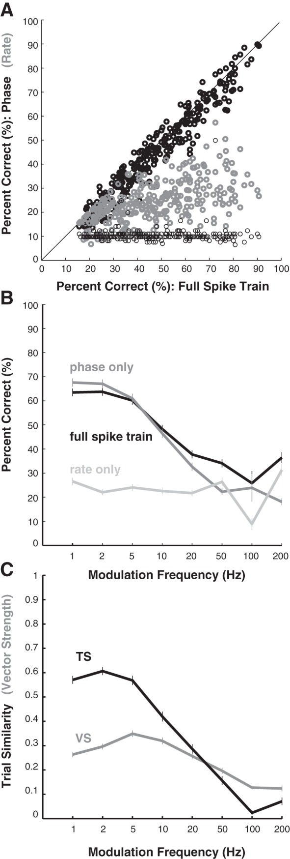
Modulation frequency discrimination. A: modulation frequency discrimination performance for the phase-only spike-train classifier (black circles) outperforms the rate-only classifier (gray circles). Performance expected by chance (based on the number of stimuli comprising each MTF) for each neuron is indicated by ordinate value of the thin black circles. B: performance of the different classifiers is shown as a function of modulation frequency by taking the average of discrimination performance for the most commonly tested modulation frequencies across all neurons in the population. C: TS and VS are plotted as functions of modulation frequency, averaged across all neurons in the population. Vertical bars on B and C indicate ±2 SE.

We computed percent correct as a function of the modulation frequency by averaging the diagonals of the confusion matrices across all neurons. The resulting curve for each classifier is shown in Fig. 10B. There was a close correspondence between the classifier performance based on the full spike train (black) and phase only (dark gray) up to roughly 20 Hz. The rate-only classifier (light gray) performed poorly but uniformly across modulation frequency. Based on this analysis, it appears that the relative utility of “temporal” vs. “rate” codes varies as a function of modulation frequency.

Population averages of TS (Fig. 10C; black curve) demonstrate that trial-to-trial reproducibility mirrors performance with the full spike train and phase-only classifiers. TS was highly correlated with percent correct for both the full spike train (r = 0.87; P < 10⁻⁸⁴) and phase classifiers (r = 0.90; P < 10⁻⁹⁹). The correlation between mean TS and the rate-only classifier was significant (P < 10⁻⁹) but substantially lower (r = 0.36). These results closely mirror those obtained for SAM (Malone et al. 2007).

Cortical responses reliably discriminate SAM and SFM signals at equivalent modulation frequencies.

Recent work indicates that cortical temporal processing can be highly dependent on the spectral content of modulated signals (Malone et al. 2013). Because we recorded SAM and SFM responses for matching CFs, carrier levels, and modulation frequencies in many cells, we could determine whether the modulation paradigm can also be decoded from cortical spike trains. To do so, we constructed composite confusion matrices (CCMs) by combining the data for SAM and SFM MTFs. For CCMs, it is possible to misclassify the modulation paradigm, even if the modulation frequency is classified correctly. For example, the response to SAM at 5 Hz might be misclassified as a response to SFM at 5 Hz. We define such errors as paradigm confusion errors. We define a correct response for a CCM as the correct identification of both the modulation frequency and modulation paradigm. Examples of CCMs for two neurons are shown in Fig. 11A. Correct responses occur along the main diagonal, and paradigm confusion errors appear along the lesser diagonals in the lower left (i.e., SAM classified as SFM) and upper right (i.e., SFM classified as SAM) quadrants. The full spike train and phase-only matrices in the top row exhibit rates of modulation paradigm errors roughly comparable to the rates of correct classifications (24 vs. 33%, and 30 vs. 33%). By contrast, the confusion matrices for a different cell depicted in the bottom row show very few modulation paradigm errors. Across all neurons (n = 186), the rates of paradigm confusion errors were generally low, as indicated by the scatterplot in Fig. 11B. Paradigm confusion error rates are indicated by small dots, which cluster near zero. The median paradigm confusion error rates were 5.8, 5.6, and 6% for the full spike train, phase-only, and rate-only classifiers, respectively. The corresponding percent correct values were 35, 32, and 14%. The full-spike-train and phase-only classifiers did not differ significantly (P > 0.18), but both significantly outperformed the rate-only classifier (P < 10⁻³²). This indicates that cortical spiking patterns, rather than average firing rates, are generally more useful in discriminating SAM and SFM.

Fig. 11.

Modulation paradigm discrimination. A: these 6 confusion matrices show results for the 3 classifiers (columns) for 2 distinct cells (rows). The numerical values on the upper right of each matrix indicate percentage correct (left), and the incidence of modulation paradigm confusion errors, cases where the modulation frequency was correctly identified but the modulation paradigm [sinusoidal amplitude modulation (SAM) or SFM] was incorrectly estimated. B: the scatterplot indicates percent correct (heavy circles), expected values for chance (light circles), and the incidence of modulation paradigm confusion errors (small dots). Confusion error rates were low, resulting in the cluster of small dots near the origin. Comparisons against the full spike train classifier for the phase-only and rate-only classifiers are shown in black and gray, respectively. C: the 3 curves indicate performance of the different classifiers for paired modulation paradigm discrimination as functions of modulation frequency. Expected values for chance are uniformly 50%, since only responses to identical modulation frequencies are compared. Vertical bars indicate ±2 SE.

It is important to consider differences in the modulation depths of the SFM and SAM signals compared in the CCMs. While the SAM signals were fully (100%) modulated, there is no precise SFM analog for 100% depth, since the modulation depth is specified in Hertz (see methods) and must be considered in the context of each neuron's frequency tuning. We attempted to choose a SFM modulation depth that produced robustly modulated responses, which typically requires a depth large enough that the SFM stimulus fully exits the neuron's response area for a portion of each modulation cycle. Since cortical responses to varying modulation depths can be discriminated from one another (Figs. 5–7), the choice of modulation depth should also affect modulation paradigm discrimination. Thus we cannot rule out the possibility that it is possible, in principle, to select a SFM modulation depth that would confound the classifiers in the context of modulation paradigm discrimination (e.g., selection of a particular off-BF CF). Subject to this caveat, our results indicate that “robustly” modulated SFM signals elicit cortical spiking patterns distinct from those elicited by “fully” modulated SAM matched in all other respects, including modulation frequency.

We were particularly interested in the discrimination of modulation paradigm as a function of frequency, because modulations are perceived differently at different modulation frequencies (e.g., fluctuation vs. roughness). We computed discrimination performance for SAM/SFM pairs at matched modulation frequencies and averaged the results over the population (Fig. 11C). In the fluctuation range (>10–15 Hz), performance of the full spike train and the phase-only classifier is similar, but the curves diverge with increasing modulation frequency. Performance for the rate classifier, by contrast, is essentially constant from 1 to 200 Hz. These results suggest that modulation paradigm discrimination increasingly relies on average firing rate information at higher modulation frequencies, as would be expected from the distribution of synchrony cutoffs (see below).

Despite the similarity between Fig. 11C and Fig. 10B, it is important to note that Fig. 10B reflects the discrimination of modulation frequency for SFM, while Fig. 11C shows modulation paradigm discrimination as a function of modulation frequency. Nevertheless, the similarities between the two sets of curves suggest that the information present in moment-to-moment changes in firing rate is available for decoding multiple stimulus features below roughly 20 Hz.

Even though most cortical neurons encode SAM and SFM differently enough to discriminate between them, that encoding is still subject to common temporal constraints. We compare the synchronization cutoff and BMFs for SAM and SFM in Fig. 12, A and B, respectively. We defined the synchronization limit as the highest modulation frequency that elicited a significant TS value; the BMF was defined as the value that produced the highest significant TS value. For plotting purposes only, we remapped nonstandard modulation frequencies used in a few cases to their nearest equivalent on the standard list (e.g., 4 to 5 Hz). The diagonal structure evident in the cutoff matrix (Fig. 11A) implies shared biophysical constraints on modulation encoding within the same neuron (Scott et al. 2011). SFM and SAM cutoff values were highly correlated (r = 0.68; P < 10⁻²⁵; nonsignificant cases were treated as zero for purposes of this analysis; excluding nonsignificant cases results in r = 0.69). SFM and SAM BMFs were also highly correlated (r = 0.77; P < 10⁻³⁶). The combination of strong correlations in cortical responses across modulation paradigm and robust discrimination of modulation paradigm, based on the same responses, indicates that cortical spike trains are sufficiently rich to distinguish multiple features of modulated signals, even in the presence of shared temporal constraints on the encoding process.

Given the recent demonstration that the spectral content of the carrier signal affected the temporal features of cortical responses (Malone et al. 2013), we also calculated the percentages of cortical neurons in our sample that exhibited significant TS (P < 0.001) for at least one tested modulation frequency. Most neurons had at least one significant TS value for both stimuli (79.6%; 191/240), while only 4.1% never exhibited significant TS for either modulation type. Neurons that synchronized to only SAM or only SFM were relatively uncommon and evenly balanced (7.1% vs. 9.2%).

Cortical spiking patterns support discrimination of multiple SFM parameters in parallel.

An important distinction between temporal codes and rate codes is their effective dimensionality: the number of bins in the PSTH used to represent the neural response effectively determines the dimension. As we showed for CF discrimination, it is possible for diverse spiking patterns to be collapsed into equivalent average firing rates (i.e., a single analysis “bin”), resulting in poor rate classifier performance. Alternatively, it is possible that, when analyzed at sufficient temporal resolution, cortical spiking patterns elicited by SFM stimuli that vary along multiple parameters could map onto distinct and dissociable regions of the analysis space (Malone et al. 2007).

In 36 cases derived from 31 neurons, we recorded responses to SFM signals that varied along more than a single parameter (e.g., modulation frequency and CF). Figure 13 consists of four CCMs obtained from four different cortical neurons using the full spike train classifier at the optimal temporal resolution. Panel A shows the CCM associated with three MDFs collected at 1, 5, and 10 Hz. Panel B shows the CCM for seven MDFs collected across CF. Panel C shows the CCM obtained for two MTFs collected at different carrier levels. Finally, panel D shows a CCM constructed for MTFs obtained at seven distinct CFs. These examples reveal that the classifiers do sometimes erroneously associate the correctly identified modulation frequency with a different carrier level (B) or frequency (D), resulting in additional structure in the CCM parallel with the main diagonal. Nevertheless, the spike trains in these examples were more likely to be assigned to the exact SFM signal that elicited them, rather than SFM signals that matched for only one parameter.

We evaluated performance in two ways. First, we determined whether the number of cases where both parameters were correctly identified significantly exceeded chance (P < 0.001) for each of the classifiers. This occurred in 33, 32, and 28 of the cases for the full-spike-train, phase-only, and rate-only classifiers, respectively. Second, we determined whether the number of cases where both parameters were correctly identified was significantly higher than the expected number of “partially correct” estimates, where only a single SFM parameter was correctly identified. Consider the CCM in panel D, based on nine-element MTFs at seven different CFs. If the modulation frequency is correctly identified, then the likelihood that the correct CF is also identified is one in seven, unless the spike train contains enough information to disambiguate both SFM parameters simultaneously. Conversely, if the CF is correctly identified, the chance of also identifying the modulation frequency is one in nine. Because there are two SFM parameters, each case (n = 36) yields two significance estimates (i.e., n = 72). For the full spike train classifier, both SFM parameters were encoded at rates significantly above chance (P < 0.001) in 56 of 72 cases, compared with 55/72 for the phase-only classifier, and 29/72 for the rate-only classifier. Thus cortical spike trains are often able to encode multiple SFM parameters in parallel, particularly when spike timing information is available, or, more precisely, when the firing rate information is measured at sufficient temporal resolution.

Spike timing information can discriminate among static tonal frequencies.

Given the consistent finding that spike timing information was crucial for discriminating among acoustic signals with dynamic frequency changes, we tested how well unmodulated tones of different frequencies could be discriminated using cortical responses. The dynamic features of “static” tones are limited to rapid amplitude changes at tone onset and offset. Although tone duration was 100 ms, we used an analysis epoch of 200 ms to include offset responses, which could also vary as a function of frequency. The effect of the analysis window is shown for an example cell in Fig. 14. Panel A shows the FTF calculated over the duration of the tone, while panel B shows the same FTF when the offset responses are included (blue line). Clearly, the apparent frequency tuning of this neuron is a function of time. As described in methods, the phase classifier is based on normalization of the vector norms of the binned spike counts. The impact of this normalization is indicated by the green line in panel B. The horizontal red line shows the effect of normalizing by total spike count. The PSTHs shown in panel C depict the raw data in the left column, data normalized by the vector norm in the middle column, and data normalized by the total spike count in the right column. Despite the normalization, the PSTH shapes in all columns clearly vary across CF, such that the balance between the onset and offset responses shifts substantially (compare 10 to 18 kHz). For this neuron, spiking patterns provided more information about stimulus identity than the spike counts averaged over a 200-ms window: phase classifier performance was 30% vs. 10% for the rate classifier. We note here that, although we report results for the vector norm-based normalization (see Malone et al. 2007), normalization by the total spike count produces essentially identical results. (The correlation coefficient for discrimination performance across all cells and all temporal resolutions was 0.99.)

Fig. 14.

Example of tone frequency discrimination. A: the FTF calculated during the presentation of static tones lasting 100 ms. B: FTFs calculated based on the first 200 ms from tone onset. The blue curve shows the raw data, the green curve shows the result of normalizing responses across frequency by the vector norm of binned spike counts, and the red curve shows the result of normalizing the responses by the total spike counts. C: the set of peristimulus time histograms corresponding to the FTFs shown in A and B. Colors match the type of data (raw or normalized) shown in B.

Results of the population analysis for each of the classifiers are shown in Fig. 15A. As was true of the CFFs, MDFs, and MTFs, the phase-only classifier significantly outperformed the rate-only classifier (Wilcoxon ranked sum; P < 10⁻²⁰; population medians of 22% vs. 15%). Effectively, the shapes of rate-normalized PSTHs contained more information about tone frequency than the averaged firing rate, even for static tones. Given the fact that the FTF is arguably the most common measurement of tuning in audition, this result is rather surprising, although it was anticipated by an analogous finding regarding the RLF for tones varying in level (Malone et al. 2010). In contrast with the results for CF, modulation depth, and modulation frequency, however, performance of the full spike train classifier (median: 26%) significantly exceeded that of the phase-only classifier (median: 22%; P < 10⁻⁶), suggesting a somewhat expanded role for average firing rates in discriminating static tones relative to modulated tones.

We also calculated discrimination performance for all possible pairs of static tones and generated a cumulative function (Fig. 15B) analogous to that in Fig. 4C. Despite the fact that discrimination performance for tone frequency was poorer than for CF, the minimum resolved differences were relatively similar. This likely reflects the fact that frequency tuning was quite sharp in many neurons, because elements of a stimulus pair which includes the FTF peak and an adjacent value on the steeply sloping portion of the FTF or two adjacent points on a steep FTF flank can be discriminated effectively by average firing rate differences alone. Thus the minimum resolved differences for tone frequency are quite similar between the full spike train and rate-only classifiers, and comparatively large for the phase-only classifier (Fig. 15B), an inversion of the relationship observed for CF (Fig. 4C). The fact that the phase-only classifier outperformed the rate-only classifier for tone frequency overall, despite the rate-only classifier's advantage for the minimum resolved difference, indicates that average firing rate differences were sufficient to distinguish a limited number of points on the FTF, likely those concentrated on the peak, while the phase-classifier successfully differentiated a wider range of PSTHs.

“Nonsynchronized rate coding” neurons are relatively rare in auditory cortex.

As in a number of prior studies (Malone et al. 2007, 2013; Yin et al. 2011), we evaluated the claim by Lu et al. (2001) that there exists a population of cortical neurons that exhibits significant changes in average discharge rates across modulation frequency (P < 0.001) but does not synchronize to the modulations themselves. For SFM, we found that only 6.7% of the neurons in our sample (19/283) met this criterion. Analogously, the number of neurons that exhibited significant (P < 0.001) modulation frequency discrimination performance for the rate but not for the phase classifier was quite small (3.6%; 10/281). Nearly nine times as many neurons exhibited significant performance for the phase but not the rate classifier (31.7%; 89/281).

Although rate tuning to modulation frequency was common (76.3% of neurons), significant synchronization to SFM, as measured by TS, was more common (87.6%), leaving relatively few neurons to qualify as “nonsynchronized.” However, we did find that a substantial number of cortical neurons (40.3%) did display significant changes in average firing rates for modulation frequencies above each neuron's TS-defined synchronization limit. Thus it seems evident that temporal codes and rate codes can coexist within the same neuron, as has been reported for SAM (Malone et al. 2007; Yin et al. 2011). We assessed how firing rate variation across modulation frequency was apportioned relative to the synchronization limit for each neuron by calculating the ratio of the dynamic range in firing rate above and below the synchronization limit to the total dynamic range. The median ratios were equivalent for the synchronized and nonsynchronized modulation frequency ranges (0.57 vs. 0.60; P > 0.4). Eliminating limit cases where neurons synchronized to either all or none of the tested modulation frequencies did not alter the result (0.70 vs. 0.65; P > 0.3). Thus firing rate differences seem to be similarly distributed above and below the synchronization limit for SFM signals.

Absolute firing rates constrain discharge rate modulation codes for SFM signals.

In this section, we explore the impact of global aspects of firing rate on the discrimination of dynamic frequency changes. Figure 16 plots the average spike count per modulation cycle for the MTFs in our data sample. The values decrease linearly when plotted on logarithmic axes, as is shown here, resulting in a typical firing rate of one spike per cycle for a 10-Hz modulation. This is quite similar to what we had reported for SAM (Fig. 6 in Malone et al. 2007) for the same neural population. As expected, the correlation between the spikes per cycle obtained with SAM MTFs and with SFM MTFs in the same neurons (n = 244) was highly significant (r = 0.57; P < 10⁻¹⁵³).

Fig. 16.

Average spike count per modulation cycle is shown for all tested modulation frequencies for all neurons in the sample. The line indicates the best linear fit to the data plotted on logarithmic axes. The expected number of spikes falls to <1 per modulation cycle at frequencies >10 Hz, which constrains the coding of SFM parameters by MPH shape at higher frequencies.

We have argued that the spike per cycle count is important because it constrains the diversity of cortical spiking patterns (Malone et al. 2007). This suggests that neurons that are capable of firing at higher rates might have an advantage in discrimination performance, since they are capable of greater discharge rate contrast. We examined this hypothesis by correlating discrimination performance with two measures of firing rate: the maximum average discharge rate, and the rate span, defined as the difference between the average rate maxima and minima on a given function (e.g., CFF, MDF, or MTF). The results of this analysis are shown in Table 1. The sets of correlations obtained for the full spike train and phase-only classifiers were highly similar, as would be expected from prior figures where they have been compared (e.g., Figs. 3, 4C, 6, 10, and 11). However, this is somewhat surprising, given that the normalization inherent in the phase-only classifier collapses the average firing-rate differences that comprise the rate span. We also found that the correlations between classifier performance and maximum rate were always lowest for the rate-only classifier. This suggests that the enhanced rate contrast available to neurons with higher firing rates is chiefly utilized for moment-to-moment firing rate changes within the modulation period, rather than for average rate differences across stimuli. The correlation between discrimination performance and the rate span was actually highest for the rate-only classifier for both CF and modulation depth discrimination. The comparatively low correlations for the full-spike-train and phase-only classifiers for CF discrimination are likely explained by the fact that changes in the carrier produced sufficiently robust changes in response phase that average rate differences across carriers were ancillary to the discrimination (Fig. 3). Correlations between the rate span and rate-only classifier performance were universally significant, as expected, since the rate-only classifier depends entirely on average firing rate differences within each tuning function.

Table 1.

Pearson's product moment correlations (and corresponding P values) between firing rate and discrimination performance for each of the different discrimination tasks and each of the classifier types

		Maximum Rate		Rate Span
Discrimination	Classifier Type	r	P <	r	P <
Carrier frequency	Full spike train	0.35	0.012	0.18	0.181
	Phase only	0.34	0.013	0.15	0.291
	Rate only	0.20	0.148	0.52	10−4
Modulation depth	Full spike train	0.49	10−11	0.51	10−12
	Phase only	0.46	10−9	0.42	10−8
	Rate only	0.28	0.0002	0.55	10−14
Modulation frequency	Full spike train	0.44	10−14	0.55	10−22
	Phase only	0.47	10−16	0.55	10−22
	Rate only	0.24	10−4	0.46	10−15
SAM vs. SFM	Full spike train	0.41	10−8	0.50	10−12
	Phase only	0.42	10−8	0.50	10−12
	Rate only	0.24	0.001	0.40	10−7

Firing rate is assessed in terms of either the maximum firing rate obtained for a particular stimulus on the relevant function (e.g., the modulation depth function), or for the span of average firing rates (i.e., maximum vs. minimum) for the relevant function. SAM, sinusoidal amplitude modulation; SFM, sinusoidal frequency modulation.

DISCUSSION

There were three major findings in the present study. First, all parameters defining the instantaneous frequency of SFM, CF, modulation depth, and modulation rate, are encoded in cortical spiking patterns. Carrier level, although less frequently tested, also appears to impact the shapes of cortical MPHs. These results corroborate the analogous finding obtained for SAM signals in the same population of neurons (Malone et al. 2007, 2010). Second, the dynamic hyperacuity reported for amplitude modulated signals (Malone et al. 2010) also extends to frequency modulated signals, in that SFM modulates firing rate far more strongly than would be predicted from the FTF measured with static tones. Third, although the encoding of SAM and SFM share similar temporal constraints (as indicated by common synchronization limits and BMFs), discrimination of the type of modulation was robust across the tested range of modulation frequency. Collectively, these findings attest to the richness of the cortical representation of dynamic signals.

Rate and temporal coding of dynamic stimulus features.

To a first approximation, CF is to SFM as carrier level is to SAM. Thus SFM responses may be predicted based on the FTF in much the same way that SAM responses may be predicted based on the RLF (Malone et al. 2010). Cortical responses to SFM signals remain anchored to the interaction between the instantaneous frequency of SFM and each neuron's underlying frequency tuning when the modulation frequency is very low (<5 Hz), since the simple FTF lookup model can predict the qualitative features of cortical MPHs. This clearly demonstrates that the majority of cortical neurons encode frequency per se, just as they encode amplitude per se (Malone et al. 2007), at least for relatively low modulation frequencies (<20 Hz). Furthermore, cortical spiking patterns elicited by SFM signals that varied along multiple parameter axes could often be successfully discriminated (Fig. 13), indicating that cortical frequency coding does not display invariances to particular stimulus features, but instead employs a “many-to-many” mapping between SFM signals and cortical response patterns.

This many-to-many mapping has a number of important implications for understanding the cortical representation of complex sounds. First, it is clear that the “temporal to rate code conversion” (Lu et al. 2001) is by no means complete within the core fields of auditory cortex. In fact, we would argue that this dichotomous formulation is not terribly useful as a conceptual framework for thinking about different encoding models. One problem is that a statistical criterion is used to enforce the dichotomy between “synchronized” and “nonsynchronized” responses, or significant and nonsignificant differences in average firing rate. It may be more useful to consider a continuum of effective “integration times” across neurons within a structure (e.g., Scott et al. 2011). Furthermore, the prevalence of “mixed-mode” neurons that exhibit significant rate coding beyond their synchronization limits revealed here and for SAM (Malone et al. 2007; Yin et al. 2011) demonstrates that single neurons could employ “multiple” codes for different stimuli. In effect, a neural code based on action potentials is always a rate code, and the relevant empirical question is the temporal resolution of the encoding process. In this view, the temporal resolution of a rate code is a measure of how quickly firing rates can change. In the context of spike train classification methods, the operant neural code in a given structure would be best characterized by the distribution of optimal temporal resolutions for discriminating among a particular stimulus set. By analogy to digital audio, neurons with the highest maximal firing rates and lowest response variability have the largest effective “bit-depth” when encoding dynamic features of ongoing sounds. This may explain a paradoxical outcome of our classifier analysis: across discrimination tasks, the performance of phase-only classifiers was more strongly dependent on maximum firing rate than was the performance of rate-only classifiers.

Spike train classification techniques capture both the reproducibility of responses to the same stimulus, and the discriminability of responses to different stimuli. As noted above, the use of classifiers at different temporal resolutions (i.e., bin widths) permitted us to parse the contributions of firing rate modulations at different temporal scales to the cortical representation of SFM. Although the native firing rate dynamics of auditory cortex vary across individual neurons, and by cortical field (Scott et al. 2011), the optimal value was generally around 10 ms similar to what has been reported for SAM signals in macaques (Malone et al. 2007, 2010) and squirrel monkeys (Malone et al. 2013). When firing rates were averaged over the duration of the analysis epoch (i.e., the rate-only classifier), however, information about stimulus identity was significantly impoverished relative to spiking patterns at the optimal temporal scale, even when we normalized for average firing rate differences across stimuli (i.e., the phase-only classifier). The discrepancy between “rate coding” and “temporal coding” varied across different discrimination types and was smallest for static tone frequency discrimination (Fig. 15), and largest for SFM CF discrimination at large depths (Figs. 3 and 4). For this reason, a given neuron should not be considered to reside at a fixed point of the temporal-to-rate coding continuum, as the relatively contribution of fine-scale temporal information may depend on the stimulus being discriminated.

Cortical neurons preferentially encode envelope dynamics.

As noted above, the second major finding of the study is the demonstration that the dynamic hyperacuity reported for amplitude modulated signals (Malone et al. 2010) also extends to frequency-modulated signals. FTF-lookup models, based on static tones, consistently underestimated the degree of firing rate modulation elicited by SFM signals, particularly at the smallest tested modulation depths. This suggests a neural code that emphasizes stimulus changes with response changes, rather than maintaining a constant mapping between firing rates and particular parameter values (Malone et al. 2002). Cortical responses are highly sensitive to stimulus context (Brosch and Schreiner 1997; Malone et al. 2002; Ulanovsky et al. 2003), which prevents stable mappings between particular stimuli and particular firing rates. Because ongoing dynamic sounds create their own context, similar underlying mechanisms may account for the dynamic hyperacuity we observed in the cortical representation of SFM.

Preferential encoding of dynamic stimulus features even extended to putatively static stimuli, such as tone bursts at different frequencies (Fig. 15A; see also Moshitch et al. 2006). Cortical neurons are particularly sensitive to the rapid envelope changes at tone onset and offset, and these envelope dynamics interact with each neuron's frequency tuning to produce a variety of PSTH shapes. This variety provides a potential basis for discriminating tone frequency even when average firing rate differences across frequency have been eliminated via normalization. The fact that the phase classifier significantly outperformed the rate classifier when discriminating static tones suggests a useful maxim for cortical processing: all acoustic stimuli are dynamic, and all dynamic signals are encoded by response dynamics.

Implications for the perception and discrimination of modulated signals.

The extent to which the central auditory system is able to utilize temporal information in spiking patterns remains an important open question (Dong et al. 2011; Lemus et al. 2009). Nevertheless, our results allowed us to estimate neurometric thresholds for modulation detection when temporal information is either included or excluded (Figs. 4, 7, and 15). Although direct comparison to psychophysical thresholds for FM detection are complicated by differences in stimulus parameters (e.g., signal duration, CF), the minimum resolved modulation depths of the most sensitive cortical neurons, as determined by spike train classification techniques, were roughly comparable to human psychophysical thresholds, particularly if the interpolated values for the neural data are compared (Fig. 7C). Byrne et al. (2013) reported that the minimum detectable frequency excursion for a 4-kHz carrier modulated at either 5 Hz or 20 Hz was roughly 16 Hz (i.e., a Δf/f of 0.004), consistent with prior reports (Byrne et al. 2012; Demany and Semal 1989; Fastl 1978; Viemeister et al. 2010). As was true of SAM (Malone et al. 2010), cortical sensitivity to FM at low modulation frequencies is preserved in the ascending auditory pathway, in contrast to the substantial loss of fidelity at the highest modulation frequencies.

The third major finding of the study was the demonstration that, although the encoding of SAM and SFM was subject to similar temporal constraints (Liang et al. 2002), discrimination of the type of modulation was robust over a substantial range of modulation frequencies. This complements a recent demonstration that changes in the spectral bandwidth of SAM signals with otherwise similar envelopes elicit distinct responses from cortical neurons (Malone et al. 2013) and indicates that the spectral and temporal features of dynamic acoustic signals are processed in a highly interdependent fashion.

The mechanism by which FM is detected and represented remains a source of debate (Ernst and Moore 2010). Although much of the psychophysical literature on FM processing has focused on the “conversion” of FM to AM (Saberi and Hafter 1995; Zwicker 1952) from a neurophysiological perspective, both AM and FM are represented by neural spiking patterns throughout the ascending auditory pathway. Despite the fact that SFM signals have commonly been used in psychophysics, neurophysiological studies have generally focused on FM sweeps (Atencio et al. 2007; Godey et al. 2005; Heil 1997; Kajikawa et al. 2008; Mendelson et al. 1993; Nelken and Versnel 2000; Qin et al. 2008; Tian and Rauschecker 2004; Trujillo et al. 2011; Zhang et al. 2011), limiting comparisons to both the psychophysical literature and to the large corpus of neurophysiological studies of SAM processing (see Joris et al. 2004 and Malone and Schreiner 2010 for review). By demonstrating that many cortical neurons effectively discriminate among SFM and SAM signals that are identical in carrier level, CF, and modulation frequency, and as similar as possible in modulation depth, our results suggest that FM is not “converted” to AM in the cortical representation.

Why should FM and AM be represented differently in central auditory structures? Most obviously, tuning for frequency and tuning for sound level are typically quite different at the level of individual cortical neurons (Brugge and Merzenich 1973; Recanzone et al. 2000; Sadagopan and Wang 2008, Scott et al. 2011). Cortical FTFs are almost universally band pass for frequency and tend to be more sharply tuned than even the most highly nonmonotonic RLFs (e.g., Joris et al. 2011). Differences in tuning to frequency and level predict distinct MPH shapes via simple lookup models (Malone et al. 2007, 2010). Some authors have attempted to “correct” for the fact that SFM signals centered on a neuron's BF are expected to produce two response peaks per modulation cycle by calculating VS at twice the modulation frequency (e.g., Liang et al. 2002). Nevertheless, it is important to note that this expectation is not related to an intrinsic difference between SAM and SFM signals, but rather between the typical shapes of FTFs and RLFs. Moreover, the fact that auditory cortex and much of the auditory neuraxis is tonotopically organized suggests that SFM signals would be encoded differently than SAM signals, since there is not a similarly organized map of sound level preference (Brugge and Merzenich 1973; Nakamoto et al. 2004; Phillips et al. 1994, 1995; Schreiner 1995; Sutter and Schreiner 1995). Thus SFM and SAM would be expected to engage populations of auditory neurons differently, which could explain why the temporal dynamics of cortical spiking patterns so often sufficed to distinguish them.

It is also important to note that, while a particular pair of SAM and SFM stimuli could elicit a similar response from a given cortical neuron, the impact of CF on the response phase (Fig. 2) implies that there will essentially always be a set of cortical neurons (e.g., those with different BFs) that respond differently to the same SAM/SFM stimulus pair, at least in the range of modulation frequencies where phase-locking to the stimulus envelopes is widespread (<20 Hz). Psychophysical results indicate that the discrimination of modulation type is most difficult when the modulation depth is low, and that modulation type discrimination requires larger depths than simply detecting the presence of modulation for either SAM or SFM (Moore and Sek 1994, 1995). Although our data reflect discrimination of effectively fully modulated SAM and SFM signals (i.e., 100% depth for SAM), the cortical sensitivity to auditory signals modulated at low depths demonstrated here and in prior work (Malone et al. 2010) suggests that fairly limited pooling across neurons could account for psychophysical performance on such tasks (Pouget et al. 2000).

Conclusions.

Our results suggest that AM and FM provide complimentary but distinct information about acoustic signals that is likely to be crucial for segmenting complex auditory scenes. Further experiments will be required to determine how concurrent AM and FM are perceived (Ozimek and Sek 1987; Sek and Moore 1994) and represented by neural systems (Ding and Simon 2009). In particular, relating details of the cortical encoding model to perception will require further characterization of how information in cortical spike trains is integrated across neurons (Johnson et al. 2012; Schneider and Woolley 2010), and over what time scales in different cortical regions (Scott et al. 2011). Nevertheless, our data clearly demonstrate that moment-by-moment changes in frequency are robustly represented in moment-by-moment changes in the firing rates of cortical neurons, particularly at the modulation rates that dominate both macaque vocalizations and human speech (Cohen et al. 2007; Elliott and Theunissen 2009; Rosen 1992), suggesting that cortical frequency coding is both dynamic and adaptive.

GRANTS

B. H. Scott was supported by National Institute of Deafness and Other Communications Disorders Grant DC-05287-01 and a James Arthur Fellowship from New York University. B. J. Malone was supported by National Institute of Mental Health Grant MH-12993-02 and a grant from the National Institute of Deafness and Other Communications Disorders (DC011843). M. N. Semple was supported by the W. M. Keck Foundation.

DISCLOSURES

No conflicts of interest, financial or otherwise, are declared by the author(s).

AUTHOR CONTRIBUTIONS

Author contributions: B.J.M. and M.N.S. conception and design of research; B.J.M. and B.H.S. performed experiments; B.J.M. analyzed data; B.J.M. and B.H.S. interpreted results of experiments; B.J.M. prepared figures; B.J.M. drafted manuscript; B.J.M., B.H.S., and M.N.S. edited and revised manuscript; B.J.M., B.H.S., and M.N.S. approved final version of manuscript.

REFERENCES

- Ardoint M, Lorenzi C. Effects of lowpass and highpass filtering on the intelligibility of speech based on temporal fine structure or envelope cues. Hear Res 260: 89–95, 2010 [DOI] [PubMed] [Google Scholar]
- Atencio CA, Blake DT, Strata F, Cheung SW, Merzenich MM, Schreiner CE. Frequency-modulation encoding in the primary auditory cortex of the awake owl monkey. J Neurophysiol 98: 2182–2195, 2007 [DOI] [PubMed] [Google Scholar]
- Banai K, Sabin AT, Wright BA. Separable developmental trajectories for the abilities to detect auditory amplitude and frequency modulation. Hear Res 280: 219–227, 2011 [DOI] [PMC free article] [PubMed] [Google Scholar]
- Brosch M, Schreiner CE. Time course of forward masking tuning curves in cat primary auditory cortex. J Neurophysiol 77: 923–943, 1997 [DOI] [PubMed] [Google Scholar]
- Brugge JF, Merzenich MM. Responses of neurons in auditory cortex of the macaque monkey to monaural and binaural stimulation. J Neurophysiol 36: 1138–1158, 1973 [DOI] [PubMed] [Google Scholar]
- Byrne AJ, Viemeister NF, Stellmack MA. The effects of unmodulated carrier fringes on the detection of frequency modulation. J Acoust Soc Am 133: 998–1003, 2013 [DOI] [PMC free article] [PubMed] [Google Scholar]
- Byrne AJ, Wojtczak M, Viemeister NF. Forward masking of frequency modulation. J Acoust Soc Am 132: 3375–3386, 2012 [DOI] [PMC free article] [PubMed] [Google Scholar]
- Cohen YE, Theunissen F, Russ BE, Gill P. Acoustic features of rhesus vocalizations and their representation in the ventrolateral prefrontal cortex. J Neurophysiol 97: 1470–1484, 2007 [DOI] [PubMed] [Google Scholar]
- Demany L, Semal C. Detection thresholds for sinusoidal frequency modulation. J Acoust Soc Am 85: 1295–1301, 1989 [DOI] [PubMed] [Google Scholar]
- Ding N, Simon JZ. Neural representations of complex temporal modulations in the human auditory cortex. J Neurophysiol 102: 2731–2743, 2009 [DOI] [PMC free article] [PubMed] [Google Scholar]
- Dong C, Qin L, Liu Y, Zhang X, Sato Y. Neural responses in the primary auditory cortex of freely behaving cats while discriminating fast and slow click-trains. PLos One 6: e25895, 2011 [DOI] [PMC free article] [PubMed] [Google Scholar]
- Elliott TM, Theunissen FE. The modulation transfer function for speech intelligibility. PLoS Comput Biol 5: e1000302, 2009 [DOI] [PMC free article] [PubMed] [Google Scholar]
- Ernst SM, Moore BC. Mechanisms underlying the detection of frequency modulation. J Acoust Soc Am 128: 3642–3648, 2010 [DOI] [PubMed] [Google Scholar]
- Fastl H. Frequency discrimination for pulsed vs. modulated tones. J Acoust Soc Am 63: 275–277, 1978 [DOI] [PubMed] [Google Scholar]
- Foffani G, Moxon KA. PSTH-based classification of sensory stimuli using ensembles of single neurons. J Neurosci Method 135: 107–120, 2004 [DOI] [PubMed] [Google Scholar]
- Gilbert G, Lorenzi C. The ability of listeners to use recovered envelope cues from speech fine structure. J Acoust Soc Am 119: 2438–2444, 2006 [DOI] [PubMed] [Google Scholar]
- Godey B, Atencio CA, Bonham BH, Schreiner CE, Cheung SW. Functional organization of squirrel monkey primary auditory cortex: responses to frequency-modulation sweeps. J Neurophysiol 94: 1299–1311, 2005 [DOI] [PubMed] [Google Scholar]
- Goldberg JM, Brown PB. Response of binaural neurons of dog superior olivary complex to dichotic tonal stimuli: some physiological mechanisms of sound localization. J Neurophysiol 32: 613–636, 1969 [DOI] [PubMed] [Google Scholar]
- Heil P. Aspects of temporal processing of FM stimuli in primary auditory cortex. Acta Otolaryngol Suppl Stockh 532: 99–102, 1997 [DOI] [PubMed] [Google Scholar]
- Johnson JS, Yin P, O'Connor KN, Sutter ML. Ability of primary auditory cortical neurons to detect amplitude modulation with rate and temporal codes: neurometric analysis. J Neurophysiol 107: 3325–3341, 2012 [DOI] [PMC free article] [PubMed] [Google Scholar]
- Joris PX, Bergevin C, Kalluri R, Mc Laughlin M, Michelet P, van der Heijden M, Shera CA. Frequency selectivity in Old-World monkeys corroborates sharp cochlear tuning in humans. Proc Natl Acad Sci U S A 108: 17516–17520, 2011 [DOI] [PMC free article] [PubMed] [Google Scholar]
- Joris PX, Schreiner CE, Rees A. Neural processing of amplitude-modulated sounds. Physiol Rev 84: 541–577, 2004 [DOI] [PubMed] [Google Scholar]
- Kaas JH, Hackett TA. Subdivisions of auditory cortex and levels of processing in primates. Audiol Neurootol 3: 73–85, 1998 [DOI] [PubMed] [Google Scholar]
- Kajikawa Y, de la Mothe LA, Blumell S, Sterbing-D'Angelo SJ, D'Angelo W, Camalier CR, Hackett TA. Coding of FM sweep trains and twitter calls in area CM of marmoset auditory cortex. Hear Res 239: 107–125, 2008 [DOI] [PMC free article] [PubMed] [Google Scholar]
- Kay RH. Hearing of modulation in sounds. Physiol Rev 62: 894–975, 1982 [DOI] [PubMed] [Google Scholar]
- Lemus L, Hernandez A, Romo R. Neural codes for perceptual discrimination of acoustic flutter in the primate auditory cortex. Proc Natl Acad Sci U S A 106: 9471–9476, 2009 [DOI] [PMC free article] [PubMed] [Google Scholar]
- Liang L, Lu T, Wang X. Neural representations of sinusoidal amplitude and frequency modulations in the primary auditory cortex of awake primates. J Neurophysiol 87: 2237–2261, 2002 [DOI] [PubMed] [Google Scholar]
- Lu T, Liang L, Wang X. Temporal and rate representations of time-varying signals in the auditory cortex of awake primates. Nat Neurosci 4: 1131–1138, 2001 [DOI] [PubMed] [Google Scholar]
- Malone BJ, Beitel RE, Vollmer M, Heiser MA, Schreiner CE. Spectral context affects temporal processing in awake auditory cortex. J Neurosci 33: 9431–9450, 2013 [DOI] [PMC free article] [PubMed] [Google Scholar]
- Malone BJ, Schreiner CE. Coding of time varying sounds: envelope modulations. In: The Oxford Handbook of Auditory Science: The Auditory Brain, edited by Rees A, Palmer A. Oxford, UK: Oxford University Press, 2010 [Google Scholar]
- Malone BJ, Scott BH, Semple MN. Context-dependent adaptive coding of interaural phase disparity in the auditory cortex of awake macaques. J Neurosci 22: 4625–4638, 2002 [DOI] [PMC free article] [PubMed] [Google Scholar]
- Malone BJ, Scott BH, Semple MN. Dynamic amplitude coding in the auditory cortex of awake rhesus macaques. J Neurophysiol 98: 1451–1474, 2007 [DOI] [PubMed] [Google Scholar]
- Malone BJ, Scott BH, Semple MN. Temporal codes for amplitude contrast in auditory cortex. J Neurosci 30: 767–784, 2010 [DOI] [PMC free article] [PubMed] [Google Scholar]
- Mardia K, Jupp P. Directional Statistics. New York: Wiley, 2000 [Google Scholar]
- Mendelson JR, Schreiner CE, Sutter ML, Grasse KL. Functional topography of cat primary auditory cortex: responses to frequency-modulated sweeps. Exp Brain Res 94: 65–87, 1993 [DOI] [PubMed] [Google Scholar]
- Moore BC, Sek A. Discrimination of modulation type (amplitude modulation or frequency modulation) with and without background noise. J Acoust Soc Am 96: 726–732, 1994 [DOI] [PubMed] [Google Scholar]
- Moore BC, Sek A. Effects of carrier frequency, modulation rate, and modulation waveform on the detection of modulation and the discrimination of modulation type (amplitude modulation vs. frequency modulation). J Acoust Soc Am 97: 2468–2478, 1995 [DOI] [PubMed] [Google Scholar]
- Moshitch D, Las L, Ulanovsky N, Bar-Yosef O, Nelken I. Responses of neurons in primary auditory cortex (A1) to pure tones in the halothane-anesthetized cat. J Neurophysiol 95: 3756–3769, 2006 [DOI] [PubMed] [Google Scholar]
- Nakamoto KT, Zhang J, Kitzes LM. Response patterns along an isofrequency contour in cat primary auditory cortex (AI) to stimuli varying in average and interaural levels. J Neurophysiol 91: 118–135, 2004 [DOI] [PubMed] [Google Scholar]
- Nelken I, Versnel H. Responses to linear and logarithmic frequency-modulated sweeps in ferret primary auditory cortex. Eur J Neurosci 12: 549–562, 2000 [DOI] [PubMed] [Google Scholar]
- Nie K, Stickney G, Zeng FG. Encoding frequency modulation to improve cochlear implant performance in noise. IEEE Trans Biomed Eng 52: 64–73, 2005 [DOI] [PubMed] [Google Scholar]
- Ozimek E, Sek A. Perception of amplitude and frequency modulated signals (mixed modulation). J Acoust Soc Am 82: 1598–1603, 1987 [DOI] [PubMed] [Google Scholar]
- Phillips DP, Semple MN, Calford MB, Kitzes LM. Level-dependent representation of stimulus frequency in cat primary auditory cortex. Exp Brain Res 102: 210–226, 1994 [DOI] [PubMed] [Google Scholar]
- Phillips DP, Semple MN, Kitzes LM. Factors shaping the tone level sensitivity of single neurons in posterior field of cat auditory cortex. J Neurophysiol 73: 674–686, 1995 [DOI] [PubMed] [Google Scholar]
- Pouget A, Dayan P, Zemel R. Information processing with population codes. Nat Rev Neurosci 1: 125–132, 2000 [DOI] [PubMed] [Google Scholar]
- Qin L, Wang J, Sato Y. Heterogeneous neuronal responses to frequency-modulated tones in the primary auditory cortex of awake cats. J Neurophysiol 100: 1622–1634, 2008 [DOI] [PubMed] [Google Scholar]
- Qin MK, Oxenham AJ. Effects of simulated cochlear-implant processing on speech reception in fluctuating maskers. J Acoust Soc Am 114: 446–454, 2003 [DOI] [PubMed] [Google Scholar]
- Recanzone GH, Guard DC, Phan ML. Frequency and intensity response properties of single neurons in the auditory cortex of the behaving macaque monkey. J Neurophysiol 83: 2315–2331, 2000 [DOI] [PubMed] [Google Scholar]
- Rosen S. Temporal information in speech: acoustic, auditory and linguistic aspects. Philos Trans R Soc Lond B Biol Sci 336: 367–373, 1992 [DOI] [PubMed] [Google Scholar]
- Ruggles D, Bharadwaj H, Shinn-Cunningham BG. Normal hearing is not enough to guarantee robust encoding of suprathreshold features important in everyday communication. Proc Natl Acad Sci U S A 108: 15516–15521, 2011 [DOI] [PMC free article] [PubMed] [Google Scholar]
- Saberi K, Hafter ER. A common neural code for frequency- and amplitude-modulated sounds. Nature 374: 537–539, 1995 [DOI] [PubMed] [Google Scholar]
- Sadagopan S, Wang X. Level invariant representation of sounds by populations of neurons in primary auditory cortex. J Neurosci 28: 3415–3426, 2008 [DOI] [PMC free article] [PubMed] [Google Scholar]
- Schneider DM, Woolley SM. Discrimination of communication vocalizations by single neurons and groups of neurons in the auditory midbrain. J Neurophysiol 103: 3248–3265, 2010 [DOI] [PMC free article] [PubMed] [Google Scholar]
- Schreiner CE. Order and disorder in auditory cortical maps. Curr Opin Neurobiol 5: 489–496, 1995 [DOI] [PubMed] [Google Scholar]
- Scott BH, Malone BJ, Semple MN. Effect of behavioral context on representation of a spatial cue in core auditory cortex of awake macaques. J Neurosci 27: 6489–6499, 2007 [DOI] [PMC free article] [PubMed] [Google Scholar]
- Scott BH, Malone BJ, Semple MN. Representation of dynamic interaural phase difference in auditory cortex of awake rhesus macaques. J Neurophysiol 101: 1781–1799, 2009 [DOI] [PMC free article] [PubMed] [Google Scholar]
- Scott BH, Malone BJ, Semple MN. Transformation of temporal processing across auditory cortex of awake macaques. J Neurophysiol 105: 712–730, 2011 [DOI] [PMC free article] [PubMed] [Google Scholar]
- Sek A, Moore BC. Detection of mixed modulation using correlated and uncorrelated noise modulators. J Acoust Soc Am 95: 3511–3517, 1994 [DOI] [PubMed] [Google Scholar]
- Shamma S, Lorenzi C. On the balance of envelope and temporal fine structure in the encoding of speech in the early auditory system. J Acoust Soc Am 133: 2818–2833, 2013 [DOI] [PMC free article] [PubMed] [Google Scholar]
- Shannon RV, Zeng FG, Kamath V, Wygonski J, Ekelid M. Speech recognition with primarily temporal cues. Science 270: 303–304, 1995 [DOI] [PubMed] [Google Scholar]
- Sheft S, Ardoint M, Lorenzi C. Speech identification based on temporal fine structure cues. J Acoust Soc Am 124: 562–575, 2008 [DOI] [PMC free article] [PubMed] [Google Scholar]
- Stickney GS, Nie K, Zeng FG. Contribution of frequency modulation to speech recognition in noise. J Acoust Soc Am 118: 2412–2420, 2005 [DOI] [PubMed] [Google Scholar]
- Strelcyk O, Dau T. Relations between frequency selectivity, temporal fine-structure processing, and speech reception in impaired hearing. J Acoust Soc Am 125: 3328–3345, 2009 [DOI] [PubMed] [Google Scholar]
- Sutter ML, Schreiner CE. Topography of intensity tuning in cat primary auditory cortex: single-neuron versus multiple-neuron recordings. J Neurophysiol 73: 190–204, 1995 [DOI] [PubMed] [Google Scholar]
- Talcott JB, Witton C, McClean M, Hansen PC, Rees A, Green GG, Stein JF. Can sensitivity to auditory frequency modulation predict children's phonological and reading skills? Neuroreport 10: 2045–2050, 1999 [DOI] [PubMed] [Google Scholar]
- Tian B, Rauschecker JP. Processing of frequency-modulated sounds in the lateral auditory belt cortex of the rhesus monkey. J Neurophysiol 92: 2993–3013, 2004 [DOI] [PubMed] [Google Scholar]
- Trujillo M, Measor K, Carrasco MM, Razak KA. Selectivity for the rate of frequency-modulated sweeps in the mouse auditory cortex. J Neurophysiol 106: 2825–2837, 2011 [DOI] [PubMed] [Google Scholar]
- Ulanovsky N, Las L, Nelken I. Processing of low-probability sounds by cortical neurons. Nat Neurosci 6: 391–398, 2003 [DOI] [PubMed] [Google Scholar]
- Viemeister NF, Stellmack MA, Byrne AJ. Detection of modulation of a 4-kHz carrier. J Acoust Soc Am 128: 1578–1581, 2010 [DOI] [PMC free article] [PubMed] [Google Scholar]
- Yin P, Johnson JS, O'Connor KN, Sutter ML. Coding of amplitude modulation in primary auditory cortex. J Neurophysiol 105: 582–600, 2011 [DOI] [PMC free article] [PubMed] [Google Scholar]
- Zeng FG, Nie K, Stickney GS, Kong YY, Vongphoe M, Bhargave A, Wei C, Cao K. Speech recognition with amplitude and frequency modulations. Proc Natl Acad Sci U S A 102: 2293–2298, 2005 [DOI] [PMC free article] [PubMed] [Google Scholar]
- Zhang X, Qin L, Liu Y, Dong C, Sato Y. Cat's behavioral sensitivity and cortical spatiotemporal responses to the sweep direction of frequency-modulated tones. Behav Brain Res 217: 315–325, 2011 [DOI] [PubMed] [Google Scholar]
- Zwicker E. Die Grenzen der Hǒrbarkeit der Amplitudenmodulation und der Frequenzmodulation eines Tones. Acustica Akust Beih 3: 125–133, 1952 [Google Scholar]