Drawing Causal Inferences Using Propensity Scores: A Practical Guide for Community Psychologists

Abstract

Confounding present in observational data impede community psychologists’ ability to draw causal inferences. This paper describes propensity score methods as a conceptually straightforward approach to drawing causal inferences from observational data. A step-by-step demonstration of three propensity score methods – weighting, matching, and subclassification – is presented in the context of an empirical examination of the causal effect of preschool experiences (Head Start vs. parental care) on reading development in kindergarten. Although the unadjusted population estimate indicated that children with parental care had substantially higher reading scores than children who attended Head Start, all propensity score adjustments reduce the size of this overall causal effect by more than half. The causal effect was also defined and estimated among children who attended Head Start. Results provide no evidence for improved reading if those children had instead received parental care. We carefully define different causal effects and discuss their respective policy implications, summarize advantages and limitations of each propensity score method, and provide SAS and R syntax so that community psychologists may conduct causal inference in their own research.

Methods for causal inference have only recently gained popularity among social and behavioral scientists, despite their potential to allow researchers to draw causal inferences with non-randomized data. Although randomized controlled trials (RCTs) are considered the gold standard for drawing causal inference in psychological research, RCTs are not always possible—or necessary—for examining causal associations (McCall & Green, 2004; West, 2009). There are many reasons why an RCT may be difficult or impossible to implement in psychological studies. For example, when assessing the impact of peers on adolescent drug use, peer behavior cannot be randomized; when using retrospective data to estimate an effect it is impossible to randomize; when implementing a treatment program for youth in the justice system, there may be ethical issues related to withholding treatment from some participants; when determining the effectiveness of a school-based intervention for reducing aggressive behavior, there may be resistance from schools to randomize and reasons that randomization may be inappropriate (Cook, 2003). Even when an RCT is feasible and carried out, issues such as treatment noncompliance can interfere with our ability to draw causal inferences about the treatment (Mercer, 2007; Sanson-Fisher et al., 2007; Stuart, et al., 2008). In all of these cases, it may be possible to draw more valid causal inferences by applying propensity score techniques to available data. The goals of this article are to: (1) introduce key concepts of causal inference in an accessible way; (2) demonstrate step-by-step how to apply propensity score techniques to estimate more valid causal effects of a community intervention (Head Start); and (3) provide SAS syntax in Appendix A (and R syntax in Appendix B) so that researchers may adopt these techniques more readily in their own work.

A Motivating Question: What is the Causal Effect of Head Start vs. Parental Care on Reading Development?

In order to illustrate the use of propensity scores in community-based research, we will use an empirical example that includes national, longitudinal data on preschool care and reading development. We will address the following general research question: “What is the causal effect of Head Start versus parental care during the preschool years on pre-reading skills in kindergarten?” In this study, children were not randomly assigned to a type of care during the preschool years; therefore, we hypothesize substantial differences (i.e., selection effects) between children whose parents qualified for and chose to send them to Head Start versus those who chose to keep their children at home, which included both Head Start eligible and ineligible children.

Propensity Scores: A Simple Tool for Drawing Causal Inference

One of the primary challenges of estimating the effect of an exposure, predictor, or treatment using data from an observational study is the issue of confounding bias. Note that we define treatment here more broadly than what is typical in intervention research. In observational data, many constructs might be considered a treatment, such as attending preschool or college, exposure to a risk factor, or divorce. Throughout the paper, treatment will refer to any predictor in the observational context about which we wish to estimate a causal effect. A confounder is a variable that predicts both the treatment and the outcome, and therefore may impair our ability to make causal inferences about the effect. In our example, confounding of the effect of Head Start versus parental care during preschool years would occur if reasons for selecting one of these arrangements (such as household income) are also associated with later reading development. Statistical adjustments for confounders historically have been made by analysis of covariance (ANCOVA; Shadish, et al., 2002), but methods involving propensity scores have recently been proposed (e.g., Rosenbaum, 2002). A propensity score is a conceptually simple statistical tool that allows researchers to make more accurate causal inferences by balancing non-equivalent groups that may result from using a non-randomized design (Rosenbaum & Rubin, 1983). Simply speaking, an individual’s propensity score is his or her probability to have received a treatment (e.g., to have attended Head Start instead of parental care), conditional on a host of potential confounding variables. The propensity score for every individual in a study can then be used to adjust for confounding in a subsequent analysis so that more plausible causal inferences may be drawn.

Several excellent tutorials on propensity score techniques have been written. Although many have focused on medical applications (D’Agostino, 1998; VanderWeele, 2006), several recent studies present the methods in the context of social and behavioral research. For example, Stuart (2010) provides a comprehensive review of different propensity score matching strategies, as well as a thorough review of available functionality in R, SAS, and Stata for conducting matching. Harder et al. (2010) presents a thorough comparison of the performance of different propensity score techniques (e.g., one-to-one matching, full matching, inverse propensity weighting). In an effort to make these techniques accessible to applied researchers, the authors provided annotated code demonstrating how to implement each approach in R. Austin (2011a) reviews different propensity score techniques (matching, stratification, inverse probability of treatment weighting, and covariate adjustment), diagnostics for determining if the propensity score model is adequately specified, variable selection for the propensity score model, and a comparison of propensity score and regression approaches for estimating treatment effects. In addition, a related paper (Austin, 2011b) illustrates the use of these methods in the context of an empirical example investigating the effect of smoking cessation counseling on later mortality among current smokers hospitalized for a heart attack. Despite these excellent reviews, however, we believe that many social and behavioral researchers would benefit from a highly accessible, practical guide to using propensity scores in empirical studies. To this end, we present a step-by-step analysis to estimate the causal effect of child care setting (Head Start vs. parental care) on reading scores in Kindergarten. We clearly define important terms used in propensity score analysis, discuss each decision point in the analysis, and provide in online Appendices all syntax for conducting the analyses demonstrated here (note that syntax is also available at http://methodology.psu.edu). With one exception (where we demonstrated using R to perform a function not available in SAS), all analyses were implemented in SAS; this syntax is shown in Appendix A. Appendix B presents syntax in R for conducting the propensity score analyses described here.

Estimating a causal effect using a propensity score approach can be summarized with four main analytic steps presented in Figure 1: (1) estimate propensity scores in a separate analysis, (2) use propensity scores to adjust for confounding, (3) assess balance, and (4) estimate the propensity score-adjusted treatment effects (i.e., estimating the effect of interest while adjusting for confounding using the propensity scores). Below we introduce an important advantage of propensity score techniques, that of defining specific causal questions, and introduce the empirical data used in the demonstration. We then describe a strategy for estimating the propensity scores (Step 1). We then describe three general strategies (weighting, matching, and subclassification) for using these scores to adjust for confounding (Step 2). Next we discuss how to assess balance across the confounders after data have been adjusted (Step 3). Finally, we present how to fit the outcome models so that causal estimates can be obtained (Step 4). We rely on the empirical example of the causal effect of Head Start vs. parental care throughout the manuscript to demonstrate each step of the analysis.

Figure 1.

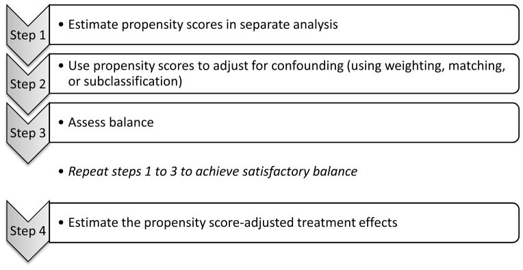
Steps to Conduct a Propensity Score Analysis

Conceptually, propensity score models are used to model selection into levels of a treatment. In our example, the propensity score model predicts Head Start enrollment from many background characteristics (i.e., potential confounders). More formally, Rosenbaum and Rubin (1983) defined the propensity score, π̂_i as the probability that individual i receives the treatment, denoted T_i, given the measured potential confounders Xi; π̂_i P(T_i = 1| X_i). These potential confounders are variables that take on their values before the intervention and thus cannot be affected by it. Propensity scores balance potential confounders in the following sense: In any subset of the population in which the propensity scores are constant, treated and untreated (i.e., Head Start and parental care) participants have identical distributions on the confounders (Rosenbaum & Rubin, 1983). Thus, differences between treatment and control individuals with the same propensity scores can be used to estimate the average effect of a treatment using observational data.

Defining Causal Questions

An important substantive advantage of propensity score approaches to causal inference is that the researcher is required to define an exact causal question. This goes beyond statements of association researchers are so accustomed to making with observational data, such as “Is mean reading ability significantly different for children who attended Head Start versus their parental care counterparts?” We draw a distinction between two primary causal questions that will be useful to psychologists. The first is the Average Treatment Effect (ATE), which simply stated is the population-level average effect of the treatment on the outcome. In the context of our example, this refers to the average causal effect of Head Start vs. parental care among all preschoolers in the study, and can be expressed more specifically as “What difference in reading development would we expect to observe if all preschool children in our study had enrolled in Head Start, compared to if all of them had received parental care?”

The second is the Average Treatment effect among the Treated (ATT), which is the effect of the treatment on the outcome among those who received the treatment. In the context of our example, this refers to the causal effect of Head Start vs. parental care among the Head Start children, or more specifically “What difference in reading development would we expect to observe if all children who attended Head Start had instead received parental care?” Very often in psychological research the ATT may be of greater interest, as it increases understanding of how exposure to a certain risk (or engagement in a certain behavior) ultimately affected those individuals who were exposed to the risk (or engaged in the behavior).

These causal questions can be further modified to address subtly different questions by, for example, redefining the sample to be analyzed. In the current study, perhaps the most policy-relevant causal effect to estimate is “Among all preschoolers who were eligible for Head Start, what difference in reading development would we expect to observe if they all attended Head Start versus if they all received parental care?” Unfortunately, in the empirical study described below, it was not possible to determine head start eligibility. Thus, we focus on the ATE and ATT described above and acknowledge that the ATT may be more informative, as the ATE addresses a question about exposure levels that are not possible for certain preschoolers. Next we introduce the empirical data used to demonstrate propensity score techniques. Wherever possible, we demonstrate how to estimate both the ATE and ATT using each propensity score approach.

The Empirical Data

Data are from the Early Childhood Longitudinal Study – Kindergarten Cohort (ECLS-K; U.S. Department of Education, National Center for Education Statistics, 2009). The current sample includes children who attended Head Start (n = 1701) or received parental care (n = 3362) prior to entering Kindergarten. Children in other types of care arrangements were not included in the analysis. Participants in the ECLS-K are a nationally representative sample of children who began Kindergarten in the 1998–1999 school year. In the fall of kindergarten, children completed a standardized assessment of reading. Demographic and family information was collected from parents in Kindergarten. The demographic characteristics are presented in Table 1. Parents were provided the following options to describe the care arrangement their children had when they were four years old: parental, relative in home, relative in another home, non-relative in home, non-relative in another home, Head Start, or center-based. Our goal is to compare expected outcomes for children who received parental care versus Head Start. As in most applied studies, our study has missing data in both the confounders and the outcome. We address missing data using multiple imputation (Allison, 2002; Little & Rubin, 2002; Schafer, 1997), and we use PROC MI to impute five data sets. SAS syntax for generating, analyzing, and combining multiple imputations appears in Appendix A. R syntax for analyzing the data appears in Appendix B.

Table 1.

Descriptive Statistics for Variables in Propensity Score Model: Head Start and Parental Care Groups.

Variables	Attended Head Start			Received Parental Care			Effect Sizes Std.
	N (Total N=1701)	Mean (%)	SD	N (Total N=3362)	Mean (%)	SD	Mean Diff.
Gender (Female)	1701	52.3%	0.50	3362	47.6%	0.50	0.10
Race (Asian)	1694	6.6%	0.25	3337	7.4%	0.26	0.03
Race (Black)	1694	36.6%	0.48	3337	11.3%	0.32	0.53*
Race (Hispanic)	1694	22.9%	0.42	3337	26.8%	0.44	0.09
Race (White)	1694	39.6%	0.49	3337	63.3%	0.48	0.49*
Child has a disability	1701	18.9%	0.39	3362	12.0%	0.33	0.18
Mother Race (Asian)	1654	6.3%	0.24	3304	6.9%	0.25	0.03
Mother Race (Black)	1654	34.8%	0.48	3304	10.3%	0.30	0.51*
Mother Race (Hispanic)	1654	21.5%	0.41	3304	24.9%	0.43	0.08
Mother Race (white)	1654	39.5%	0.49	3304	63.6%	0.48	0.49*
Mother was married at child’s birth	1515	44.4%	0.50	3146	71.0%	0.45	0.54*
Mother worked before child entered kindergarten	1572	60.3%	0.49	3236	52.7%	0.50	0.16
Mother Education (categorical)	1673	3.16	1.36	3327	3.57	1.69	0.30*
Family Type (two parent)	1621	60.5%	0.49	3294	82.7%	0.38	0.45*
Family size	1701	4.90	1.81	3362	4.93	1.56	0.02
Mother employed more 35 hours	1701	34.5%	0.48	3362	24.6%	0.43	0.21*
Mother looking for work	1701	10.1%	0.30	3362	5.3%	0.22	0.16
Mother not in labor force	1701	35.3%	0.48	3362	49.4%	0.50	0.30*
Home language (English)	1697	80.8%	0.39	3354	78.0%	0.41	0.07
Below poverty line	1701	46.7%	0.50	3362	26.1%	0.44	0.41*
Socio-economic status (SES; categorical)	1701	1.94	1.08	3362	2.60	1.37	0.61*

^*Standardized effect sizes greater than 0.2.

Step 1: Estimate Propensity Scores

Propensity score estimates are typically obtained by logistic or probit regression of the treatment on the potential confounders, although more flexible alternatives such as generalized boosted modeling (GBM; McCaffrey et al., 2004) and classification and regression trees (CART; Luellen et al., 2005) have also been applied. We will focus on the use of a logistic regression model to obtain each individual’s propensity score, and draw comparisons between logistic regression- and GBM-based results in the Discussion. In this example, the probability of attending Head Start is predicted from a large set of confounders using binomial logistic regression. An important practical issue that arises in this first step is the selection of potential confounders to include in the propensity model. All measured confounders that are predictive of selection into the treatment groups and the outcome should be included in the propensity model. Confounders for the propensity model should not be selected solely on the basis of statistical significance in predicting the treatment. Rather, standardized mean differences in covariate values across treatment and comparison conditions should be used either alone or in conjunction with significance tests. Using standardized mean differences, calculated as the difference in the proportions/means across the treatment groups divided by the standard deviation within the treatment group (Stuart, 2010), are preferable to significance testing for assessing balance on the confounders due to the potential for changes in power to affect p-values (Imai, King, & Stuart, 2008; Rosenbaum & Rubin, 1985). In addition, measures of constructs that are theoretically related to selection and the outcome should be included, regardless of statistically significant differences between the groups. Confounders that may have been influenced by the treatment (i.e., post-treatment confounders) should not be included in the propensity model (Rosenbaum, 1984). Instrumental variables, variables strongly related to the treatment but not related to the outcome, should also not be included (Pearl, 2010; Brookhart et al., 2006).

The primary assumption underlying the use of propensity scores is that all confounders of treatment selection and the outcome have been measured and included in the propensity model. Although we can never know for sure whether there is an unmeasured confounder or not, the more measured confounders that have been included, the more plausible the assumption. For example, including a few demographic variables in an ANCOVA model is most often not sufficient (Steiner, et al., 2010). In addition, if there is an unmeasured confounder that is highly correlated with a measured confounder, then including the measured confounder in the propensity model will mitigate the bias of the treatment effect estimate to the degree that they are correlated. Once the confounders have been selected and the logistic regression model is fit, the propensity score estimates are simply the predicted probabilities from the logistic regression. The goal is to obtain the best possible balance between treatment groups in terms of all pretreatment confounders; this important issue is presented in Step 3 below.

Table 1 lists all variables that were included as predictors of Head Start vs. parental care in the propensity score model (i.e., all confounders). Variables with standardized mean differences greater than .2 prior to adjustment, as well as those with a theoretical rationale for a relation to child care condition and reading development, were included in Step 1. Prior to assessing balance, it is important to assess the degree to which the distribution of propensity score estimates overlap between treatment groups; the overlapping range is commonly referred to as the region of common support. Overlapping distributions means that there are individuals in the treatment group that are similar to those in the control group on the potential confounders. When distributions do not overlap, causal inferences are not warranted because the necessary extrapolation results in unstable estimates of effects (King, 2006). We examined overlap of the propensity score distributions for Head Start and parental care groups to determine if an attempt at causal inference could be justified in this study. Findings were very similar across imputations, thus for brevity only results based on the first imputation are presented. Figure 2 includes boxplots and histograms that indicate substantial overlap of the propensity scores. For example, the boxplots show that for nearly all individuals in the Head Start group, an individual in the parental care group has a similar propensity score, and vice versa. Thus, we proceeded to the next important step in a causal analysis: using the estimated propensity scores to adjust for confounding.

Figure 2.

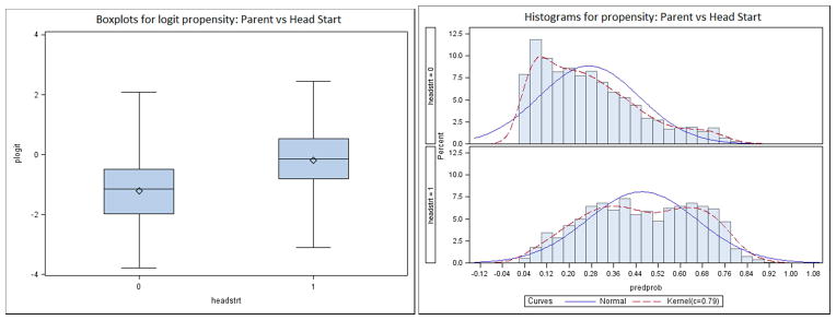
Box Plots and Histograms Showing Overlap of Propensity Score Distributions for Head Start versus Parental Care (Imputation 1).

Step 2: Use Propensity Scores to Adjust for Confounding

The second step is to adjust for confounding. We introduce and demonstrate three main techniques for adjusting for confounding using propensity score weights: inverse probability of treatment weighting (IPTW; Hirano & Imbens, 2001), matching (Rosenbaum & Rubin, 1985), and subclassification (Rosenbaum & Rubin, 1984). For all three approaches, the outcome analysis need only include the treatment indicator as a predictor; the propensity scores and any of the individual confounders are not typically included in the model (with the exception of doubly-robust methods, see e.g., Schafer & Kang, 2008). Rather, the adjustment for confounding is made by adjusting the data using the weights, matched data set, or strata, respectively.

Inverse Probability of Treatment Weighting (IPTW)

The basis for IPTW is similar to that of survey weights: there is an underrepresentation of those who are in the treatment group and have a low propensity score and an overrepresentation of those who are in the treatment group and have a high propensity score. Thus, a solution is to up-weight those who are underrepresented and down-weight those who are overrepresented. Since the propensity score, π̂, is the estimated conditional probability of receiving the treatment, the ATE is calculated by assigning those in the treatment group a weight of 1/π̂ and those in the control group a weight of 1/(1 − π̂). To calculate the ATT, those in the control group are weighted to resemble the treated population, and the treatment group is not weighted since it is already representative of the treated population; therefore for ATT, those in the treatment group are given a weight of 1, and those in the control group are given a weight of π̂/(1 − π̂). More technical details of weighting may be found in Hirano and Imbens (2001).

Matching

This approach usually involves matching one individual from the treatment group to one or more individuals in the control group. There are numerous algorithms for matching individuals based on propensity score estimates. We will limit our presentation to two of the most common ones: nearest neighbor and optimal matching. Nearest neighbor is the most popular matching technique among applied scientists, although optimal often achieves better balance (Harder et al., 2010). Regardless of the matching algorithm, matching may be done with or without replacement, although without replacement is more common. In matching without replacement, individuals may be matched only once. In matching with replacement, an individual – typically from the control group – is available to be matched to more than one treatment individual. In our demonstration, we will match without replacement. For matching control individuals to the treated individuals, the ATT is simply the mean difference between the treatment groups in the matched dataset. Currently, no method exists to estimate the ATE using matching. More technical details about matching may be found in Stuart (2010).

In nearest neighbor matching, the individuals in the treatment group are randomly sorted. The first individual in the treatment group is then matched with the individual with the closest propensity score estimate from the control group. This matched pair is set aside. The next individual is taken from the treatment group and the individual with the closest propensity score estimate from the control group is chosen as a match. This process continues until each individual from the treatment group has been matched with an individual from the control group. Any remaining individuals in the control group are discarded. Nearest neighbor matching does not minimize the overall distance (the sum of squared distances) between all matched pairs. Once a match is made, it is not revisited.

Optimal matching minimizes the overall distance by allowing previous matches to be broken and re-matched if doing so will minimize the overall distance in the propensity scores between all matched pairs. Because optimal matching minimizes the overall distance, it often results in better balance on the confounders than nearest neighbor matching.

If there are some individuals in the treatment group that are not similar to anyone from the control group based on the propensity score, then it may be beneficial to use a caliper, which limits potential matches to those within a certain range of the treated individual’s propensity score. If there are no individuals from the control group with a propensity score within the caliper for a given individual from the treatment group, then that treated individual would be excluded from analyses.

A variation of either of these matching procedures, particularly if there are many more individuals in the control group than the treatment group, is to do 1:k matching in which an individual in the treatment group is matched with k (e.g., 2) individuals in the control group. Each control individual is then weighted by 1/k. The ratio may also vary across individuals, such that one treatment group member may be matched to two control group members and another treatment group member may be matched to three control group members and so on. For our demonstration, we will use 1:1 matching. That is, we will match one control individual with one treatment individual. See Stuart (2010) for a broader discussion of matching techniques (e.g., matching with or without replacement, matching within calipers, 1:k matching).

Subclassification

Subclassification refers to dividing subjects into strata based on percentiles of the propensity scores. These percentiles may be based on the distribution of the propensity scores in the whole sample or in only the treatment group. Generally, five or six strata have been recommended (Rosenbaum & Rubin, 1984). Within each stratum, there must be individuals from each treatment group. Subclassification can be viewed as a coarsened form of matching in which, for a given stratum, individuals in the treatment group are matched with those in the control group.

Step 3: Assess Balance

Regardless of whether one plans to use weighting, matching, or subclassification for the outcome analysis, balance on the potential confounders across the treatment groups should be assessed, with a goal of determining whether differences between the treatment groups remain on the measured confounders after the data are adjusted using propensity scores. First, we give an overview of assessing balance that is applicable to weighting, matching and subclassification, and then we describe how to assess balance specifically for each technique.

Balance has often been assessed by testing whether there are statistically significant differences between the treatment groups in terms of their distributions on the confounders. For example, a t-test could be used for continuous confounders and a chi-square test could be used for categorical confounders. If there are a large number of confounders, however, some of these tests could be significant by chance. In addition, if the sample size is large, even small differences may be statistically significant. Therefore, it is recommended that the standardized mean differences be reported (Rosenbaum & Rubin, 1985). These differences should be reported for the original sample (before propensity scores are estimated, as in Table 1) and after the data are adjusted using the propensity scores.

Treatment groups are considered to be balanced on the measured confounders if standardized mean differences are less than about .2 (in absolute value) after adjustment. The standardized mean difference of .2 is often used because it is considered a small effect size (Cohen, 1988). According to this rule of thumb, if the differences are less than .2 for all measured confounders, then balance has been achieved and the next step is to conduct the outcome analysis. If some of the differences are larger than .2, then balance has not been fully achieved; in this case, the model used to estimate propensity scores can be reconsidered. For example, interactions among the unbalanced confounders, squared or cubic terms for the unbalanced confounders, or additional confounders may be added to the propensity model. The propensity scores are re-estimated, an adjustment using the propensity scores is made, and balance is re-assessed. Thus, Steps 1 through 3 can be repeated iteratively until balance is achieved. It should be noted that this process balances the groups only on measured confounders that are included in the propensity model. It does not guarantee balance on measured confounders excluded from the propensity model or on any unmeasured confounders. A sensitivity analysis can be conducted to assess the potential bias in the causal effect estimate introduced by unmeasured confounders (e.g., Imbens, 2003), although this topic falls outside the scope of the current demonstration.

Each propensity score method requires a slightly different approach to assess post-adjustment balance. For IPTW, standardized mean differences are computed on the weighted sample (see Appendix A for SAS syntax and Appendix B for R syntax). When using any matching algorithm, once the matched dataset has been created (i.e., all unmatched individuals are removed from the dataset), then balance is simply assessed by calculating the standardized mean differences between the treatment groups on each of the potential confounders. When using subclassification, balance should be assessed within each stratum. That is, standardized mean differences between the treatment and control groups on each of the potential confounders should be calculated within each stratum. Researchers may try various propensity score methods in order to identify the method that achieves optimal balance on the full set of covariates, and apply propensity scores derived from that method in the outcome model (Step 4).

In the empirical example, we adjusted for confounding using weighting, nearest neighbor matching, optimal matching, and subclassification; we then assessed balance in each of the five imputed data sets. For brevity, Table 2 presents the standardized mean differences between children in Head Start and parental care on each of the confounders for the first imputed dataset. Differences greater than .2 are denoted with an asterisk. As is evident from these diagnostics, balance on the measured confounders has been achieved using weights for the ATE as well as the ATT. Balance was not achieved on race (Black) for either matching algorithm, although the standardized mean differences are much lower than in the original unadjusted data (.31 for nearest neighbor and .32 for optimal, vs. .53 for unadjusted). Balance diagnostics are presented for each of the five quintiles for subclassification. Interestingly, balance was fully achieved for Strata 2 – 5 but not for Stratum 1 (children least likely to attend Head Start given their confounders). As noted by Steiner et al. (2010), it is often difficult to achieve balance on all confounders within each stratum. It is possible to revisit and re-estimate the propensity model until better balance is achieved across all five strata, or to attempt to achieve better balance using a doubly robust method (Schafer & Kang, 2008); however, for illustration and comparison purposes we will estimate the causal effect given the balance in Table 2.

Table 2.

Balance Table: Standardized Mean Differences for Subclassification, Weighting and Matching for Imputation 1.

Confounder	Unadjusted	Weighting		Matching		Subclassification Stratum
		ATE	ATT	Nearest Neighbor	Optimal	1	2	3	4	5
Gender (Female)	0.10	0.00	0.00	0.03	0.02	0.07	0.13	0.08	0.06	0.12
Race (Asian)	0.03	0.00	0.01	0.04	0.05	0.08	0.07	0.02	0.06	0.14
Race (Black)	0.53*	0.00	0.01	0.31*	0.32*	0.10	0.02	0.01	0.03	0.07
Race (Hispanic)	0.09	0.04	0.02	0.19	0.13	0.28*	0.18	0.04	0.15	0.09
Race (White)	0.49*	0.03	0.02	0.17	0.20	0.24*	0.12	0.01	0.05	0.07
Child has a disability	0.18	0.00	0.01	0.05	0.03	0.13	0.05	0.04	0.09	0.01
Mother Race (Asian)	0.03	0.00	0.01	0.04	0.05	0.06	0.06	0.01	0.04	0.10
Mother Race (Black)	0.51*	0.01	0.00	0.32*	0.32*	0.11	0.07	0.03	0.00	0.11
Mother Race (Hispanic)	0.08	0.04	0.02	0.18	0.14	0.32*	0.19	0.04	0.15	0.15
Mother Race (white)	0.49*	0.03	0.02	0.17	0.20	0.28*	0.11	0.01	0.08	0.01
Mother was married at child’s birth	0.54*	0.01	0.00	0.15	0.16	0.07	0.10	0.01	0.03	0.07
Mother worked before child entered kindergarten	0.16	0.00	0.02	0.08	0.05	0.00	0.01	0.04	0.02	0.09
Mother education (categorical)	0.30*	0.03	0.02	0.07	0.04	0.27*	0.11	0.00	0.11	0.05
Family type (two parent)	0.45*	0.00	0.00	0.19	0.18	0.01	0.02	0.10	0.04	0.12
Family size	0.02	0.01	0.03	0.03	0.02	0.11	0.03	0.05	0.06	0.13
Mother employed more 35 hours	0.21*	0.00	0.01	0.08	0.07	0.09	0.05	0.01	0.10	0.16
Mother looking for work	0.16	0.01	0.04	0.06	0.05	0.12	0.07	0.11	0.06	0.16
Mother not in labor force	0.30*	0.01	0.00	0.11	0.08	0.01	0.01	0.01	0.02	0.06
Home language (English)	0.07	0.05	0.02	0.19	0.15	0.42*	0.19	0.10	0.12	0.15
Below poverty line	0.41*	0.00	0.00	0.06	0.06	0.07	0.17	0.12	0.00	0.04
Socio-economic status (SES; categorical)	0.61*	0.02	0.01	0.00	0.03	0.31*	0.12	0.08	0.09	0.04

^*Standardized effect sizes greater than 0.2.

Step 4: Estimating the Propensity Score-Adjusted Treatment Effects: Causal Effects of Head Start vs. Parental Care

Once balance is deemed sufficient on the set of confounders, the causal effects of the treatment can be assessed using the propensity score-adjusted data. For IPTW, weights (either the ATE or the ATT weights, depending on the causal question) are applied to the general linear model predicting reading scores from an indicator of Head Start vs. parental care in the same manner as survey weights. For matching, the causal effect of the treatment on the outcome is estimated using a general linear model predicting reading scores from an indicator for Head Start vs. parental care among the final matched sample. For subclassification, the estimated effect of type of care on reading scores and corresponding standard error are estimated within each stratum, and the weighted average computed across the strata. When estimating the ATE, the weight used for each stratum should be the proportion of sample subjects in the given stratum; when estimating the ATT, the weight used for each stratum should be the proportion of treated subjects in the given stratum.

In the empirical example, for each of the five imputed data sets, we estimated propensity scores, used them to adjust for confounding, assessed balance, fit the outcome models, and then combined the causal effect estimates across imputations using Rubin’s rules (Little & Rubin, 2002; Schafer, 1997). For IPTW, SAS PROC GENMOD was used to obtain robust standard errors. For matching and subclassification, the outcome model used in this demonstration was a t-test. For the subclassification technique, the t-test was performed for each stratum, and weighted averages of the estimated mean differences and standard errors were computed across strata.

Table 3 presents the estimated causal effects of Head Start versus parental care for each method; the first three columns correspond to different available approaches to estimate the ATE, whereas the last three columns correspond to different available approaches to estimate the ATT. First we turn our attention to the ATE. The unadjusted comparison showed that on average, children who received parental care significantly outperformed children who attended Head Start on reading in Kindergarten (estimate = −3.62, p < .001). We then ran an ANCOVA model controlling for basic demographic variables – child’s gender and race, mother’s education, and socio-economic status. Although the strength of the difference weakened to less than half (estimate = −1.57, p < .001), children who received Head Start still scored significantly lower than children who had parental care. Both weighting and subclassification approaches to estimate the ATE supported this same conclusion, although the effects were even weaker (weighting estimate = −1.46, p = .004; subclassification estimate = −1.39, p = .003). In sum, our best estimate of the difference in the population average reading score if the entire population attended Head Start, compared to if they all received parental care, is roughly 1.4 units lower if they attended Head Start. Regardless of the propensity score technique used, this mean difference was statistically significant. We note, however, that the ATE may not correspond to a meaningful question in this example, as many children who received parental care would not have been eligible for Head Start.

Table 3.

Estimates of the Causal Effect of Head Start vs. Parental Care.

	ATE			ATT
Method	Estimate	Std. Error	p-value	Estimate	Std. Error	p-value
Unadjusted	−3.62	0.30	<0.001	---	---	---
ANCOVA including four covariatesa	−1.57	0.31	<0.001	---	---	---
Weighting	−1.46	0.51	0.004	−0.35	0.42	0.402
Matching – nearest neighbor	---	---	---	−0.24	0.41	0.562
Matching – optimal	---	---	---	−0.34	0.40	0.389
Subclassification	−1.39	0.45	0.003	−0.31	0.38	0.413

Notes. Estimates greater than zero indicate higher mean reading score in Head Start group. Dashed lines indicate that effect is not applicable.

^aCovariates included were child’s gender, child’s race, mother’s education and socio-economic status

The absence of estimates for the ATT using unadjusted and ANCOVA models emphasizes a key feature of using propensity score techniques: the causal question must be defined a priori. A more policy-relevant question, and a more logical one in this case, is the average effect of Head Start versus parental care among children who attended Head Start. All four propensity score techniques – weighting, nearest neighbor matching, optimal matching, and subclassification – produced nearly identical estimates, all providing no evidence for a causal effect (range of estimate = −0.35 to −0.24, range of p = .40 to .56). In other words, regardless of the exact technique used to adjust for the many confounders, children who attended Head Start would not be expected to perform any better on reading had they instead received parental care. In sum, the exact technique used to adjust for the large selection effects evident in Table 1 did not impact the conclusions about the causal effect of Head Start versus parental care, but the specific causal question to be addressed (ATE vs. ATT) was critical to the implications.

Discussion

In this study, substantial confounding created the potential for bias: parents who sent their child to Head Start differed considerably at baseline from those who provided parental care. To the extent that those baseline characteristics predicted both selection into Head Start versus parental care and reading development, the estimated effect of preschool setting on reading development will be biased. Without the use of propensity scores, we would have concluded that children receiving parental care would have significantly better reading scores in kindergarten than those attending Head Start; however, this is largely the result of a selection bias whereby children who received parental care also came from more advantaged families (see Table 1).

The inclusion of four well-documented potential confounders (child’s gender, child’s race, maternal education, and socioeconomic status) weakened the estimated association considerably, from −3.62 to −1.57. By including propensity scores to estimate the ATE, in this particular study we reached a similar conclusion to that based on ANCOVA; the more extensive set of potential confounders included in the propensity score model suggested an even weaker effect of −1.46 for IPTW and −1.39 for subclassification (we note that matching cannot be used to estimate the ATE). Despite the many confounders that had large standardized mean differences pre-adjustment, including only the four primary confounders in the ANCOVA did a fairly good job at adjusting the estimate. This may be partly due to child’s gender, child’s race, maternal education, and socioeconomic status being correlated with the additional confounders that were included in the propensity score model. Regardless, because the ANCOVA model makes the (likely too restrictive) assumptions that 1) the outcome is linearly related to each confounder, and 2) the difference in the mean on the outcome for the treatment groups does not vary with any of the covariates, we recommend a propensity score-based approach to estimating an ATE from observational data. We refer readers to Schafer and Kang (2008) for an excellent presentation of issues related to using ANCOVA to estimate causal effects.

Most notable in Table 3 is the fact that the standard method for adjusting for selection effects, ANCOVA, estimates the impact of Head Start compared to parental care overall, as opposed to estimating the impact among children who actually enrolled in (and thus qualified for) Head Start. When the causal question is redefined in this way, all four propensity score approaches demonstrated here suggest the same thing: even with this large sample, we found no evidence to expect better or worse reading ability if that group of children had instead received parental care.

It should be noted that propensity scores will not always yield results that differ from unadjusted models. For example, using a different data set that compared children who had received one versus two years in preschool, we found that in both the unadjusted and adjusted models, regardless of the propensity score technique used, the treatment effect was positive and statistically significant (for more information about the preschool program, see Rhoades, et al., 2010). We concluded that an additional year of preschool has a significant positive effect on kindergarten vocabulary. There appeared to be very minimal bias due to confounding, suggesting that children of parents who received two years of preschool beginning at age 3 did not differ from those who received one year of preschool beginning at age 4. Even though all models yielded similar results, had we not estimated the propensity score model we could not have determine that there was no measured confounding, and therefore could not have inferred causality.

Although different propensity score techniques provide similar results for the ATE and ATT, respectively, it is natural to consider how one should choose from the set of available techniques. Advantages and disadvantages of each technique are presented below. One argument is to choose the method that obtains the best balance (e.g., Harder, et al., 2010). In applied situations, it is possible that balance is achieved using certain methods but not others; thus, balance should be considered in selecting a method. However, achieving balance on the measured confounders means that bias due to those confounders is removed; bias due to unmeasured confounders may still exist. Nevertheless, it provides a useful benchmark and point of departure for sensitivity analyses (Rosenbaum, 2002). Even more fundamental than the choice of propensity score technique, however, is the fact that one must first define the exact causal question to be addressed. As demonstrated here, the ATE is not as policy-relevant, and may not be very meaningful. The ATT, however, addresses a substantively important question.

Advantages and Limitations of Each Propensity Score Technique

IPTW

Once propensity scores are obtained, weighting is relatively easy to implement in statistical packages that can incorporate sampling weights. In addition, it is straightforward to include other variables such as moderators in the outcome analysis. A limitation of IPTW is that very large weights can cause estimation problems. A π̂ near zero in the treatment group or near one in the control group can lead to problems because the inverse propensity is very large. To help remedy this problem, weights are often stabilized. One way to stabilize the weights is to use the mean propensity score for the treatment group and one minus the mean propensity score for the control group in the numerator of the weights rather than one. If after stabilization, some of the weights are very large due to propensity scores estimated near zero or one, weights may be trimmed (e.g., weights less than .10 could be set equal to .10 and weights greater than 10 could be set equal to 10), although this approach is ad hoc (see Potter, 1993 for a discussion on weight trimming). The best course of action may be to choose a different propensity score technique.

Matching

When the ATT is of interest, matching is an intuitive approach to causal inference, in that similar people (in terms of their propensity scores) from the treatment and control groups are paired so that a direct comparison can be made between groups. A disadvantage of matching, however, is that some of the control observations are usually thrown away, although this can be mitigated to some extent by 1:k variable ratio matching. Another feature of matching that may be a disadvantage in some cases is that one treatment group must be selected and the other group is then matched to that group. The treatment effect then represents an estimate for the selected group only, not the full population. Often researchers are more interested in the average treatment effect among the treated (ATT) than the treatment effect among the untreated. In this case, ideally the control group propensity scores should completely overlap those of the treatment group. To ensure that this happens, the researcher generally needs many more control individuals than treated individuals. If some treatment individuals must be removed from the sample because they do not have appropriate matches in the control group, then the effect estimated is no longer the ATT; rather, it is the average treatment effect among a subset of the treated (the matched individuals). If there are fewer control individuals than treated individuals or if the control group propensity scores do not completely overlap those of the treatment group, it may be best to use a technique other than matching.

Subclassification

A primary advantage of subclassification is its ease of use. The researcher divides the sample into quintiles based on the propensity scores, estimates the treatment effect in each quintile, and takes the weighted average of the estimates. Thus, subclassification does not require the more complex algorithms that matching requires. Also, unlike some matching algorithms, such as 1:1 nearest neighbor and optimal, subclassification does not throw away any of the control observations. The primary disadvantage of subclassification is that balance should be assessed and ideally achieved within each stratum; this can prove to be more difficult in practice than obtaining balance overall.

Propensity score as a covariate

It may be tempting to attempt to control for confounding using the simplistic approach of including propensity scores as a single covariate in the outcome analysis. When compared to including all of the potential confounders individually as covariates in a regression or ANCOVA, this technique has a substantial advantage, in that the large number of potential confounders is reduced to a single numerical summary. Although it is easy to implement, this method has several important limitations and thus was not considered in the present study. First, there is no way to check balance; in fact, the underlying statistical theory regarding balance does not apply to this technique (see Stuart, 2010 for further explanation). Second, because the propensity score is included in the outcome model, the interpretation of the causal effect based on this technique is the effect conditional on the propensity score, and requires the assumption that the outcome is linearly related to the propensity score. Because of these limitations we do not recommend using propensity scores as a covariate.

Computational Limitations of SAS

It should be noted that, unlike R, there are some limitations related to using SAS for propensity score analysis. First, to our knowledge, estimating propensity scores by GBM or CART is not possible in standard SAS, which is why we focused our demonstration on logistic regression-based propensity scores. However, GBM and other machine learning methods have been shown in some cases to perform better than logistic regression in simulation studies (Luellen et al., 2005; Lee et al., 2009). Thus, we have included in Appendix B sample R syntax for estimating the propensity scores using GBM. We note that in this example, logistic regression- and GBM-based propensity scores were correlated between .93 and .96 across imputations, thus results using these approaches are essentially identical. Second, we did not illustrate the technique of full matching, a matching algorithm that has been shown in simulation studies to outperform other matching algorithms in terms of balance (see, e.g., Stuart & Green, 2008). To our knowledge, there is no SAS macro that will implement the full matching algorithm. Despite these current limitations, we believe the SAS-based approaches demonstrated here will help to facilitate broad use of propensity score methods so that social and behavioral researchers can draw more valid causal inferences than can be drawn using standard data analytic techniques.

Conclusions

In conclusion, we have illustrated the use of propensity score methods to assess the causal effect of different preschool arrangements on later reading ability. We found that the estimates of the causal effect for the full population, based on weighting and subclassification, were similar to the estimate based on a more standard ANCOVA model. All of these suggest that parent-based care is expected to produce better verbal ability on average, although the effect is less than half that from the model that is not adjusted for any potential confounders. We then demonstrated that a different causal effect, corresponding to the causal effect of Head Start versus parental care among those who actually enrolled in Head Start, is more logical and has better policy relevance. The estimates of the causal effect for this important subpopulation (Head Start students), based on weighting, matching, and subclassification, all suggest no evidence for an improvement or detriment in later reading ability for these children due to their preschool arrangement. Finally, we discussed advantages and limitations of each propensity score method. When choosing among the methods, consideration should be given to the issue of balance, and in particular to the specific causal question that is being addressed.

Appendix A. SAS Syntax for Conducting Propensity Score Analysis

Note: Words that are italicized and in brackets (e.g., [variable]) indicate places to insert datasets or variable names for the specific analysis. All other syntax can be copied and pasted.

1. Multiple Imputation to Handle Missing Data

proc mi data= [dataset] out=propmi nimpute=5 seed=25;
 em converge=1E-3 maxiter=500;
 var [covariate list, treatment, outcome];
run;

2. Estimate Propensity Scores Using Logistic Regression

proc logistic data=propmi descending;
 class [treatment];
 model [treatment] = [covariate list]/link=logit rsquare;
 by _imputation_;
 output out=predin predicted=predprob;
run;
*predprob is name of propensity score variable;

3. Check Overlap of Propensity Scores

proc sort data=predin; by _imputation_ [treatment]; run;
proc boxplot data=predin;
 by _imputation_;
 plot plogit*[treatment];
 title ‘Boxplots for logit propensity: Head Start vs Parent’;
run;
proc univariate data=predin normal;
 class [treatment];
 var predprob;
 by _imputation_;
 histogram /normal kernel;
 title ‘Histograms for propensity: Head Start vs Parent’;
run;

4. Separate Data Sets by Imputation

data data1 data2 data3 data4 data5;
 set predin;
 if _imputation_ = 1 then output data1; else
 if _imputation_ = 2 then output data2; else
 if _imputation_ = 3 then output data3; else
 if _imputation_ = 4 then output data4; else
 if _imputation_ = 5 then output data5;
run;

5. Assess Balance (For One Imputation)

*Estimate Standardized Mean Differences;
*For weighting: add a weight statement in both means procedures;
*For matching: replace [dataset] with the matched dataset;
proc means data=[dataset](where=([treatment]=0));
 var [covariate list];
 output out=baltx1(drop=_FREQ_ _TYPE_);
run;
proc transpose data=baltx1 out=tbaltx1(rename=(_NAME_=NAME));
 id _STAT_;
run;
proc means data=[dataset](where=([treatment]=1));
 var [covariate list];
 output out=baltx2(drop=_FREQ_ _TYPE_ );
run;
proc transpose data=baltx2 out=tbaltx2(rename=(_NAME_=NAME) rename=(MEAN=M2)
rename=(STD=STD2) rename=(N=N2) rename=(MIN=MIN2)   rename=(MAX=MAX2));
 id _STAT_;
run;
proc sort data=tbaltx1;
 by NAME;
run;
proc sort data=tbaltx2;
 by NAME;
run;
data bal;
 merge tbaltx1 tbaltx2;
 by NAME;
run;
data bal;
 set bal;
 stdeff=(M2-MEAN)/STD2;
run;
proc print data=bal;
 var name stdeff;
run;
*Estimate Standardized Mean Differences within Quintiles for
Subclassification;
*gen2 macro available at http://methodology.psu.edu/;
*strat macro available at http://methodology.psu.edu/;
%gen2(strat1,[treatment],[individual covariate],0); run;
data final;
 set final_[covariate1] final_[covariate2] final_[covariate3]
final_[covariate4]    final_[covariate5] final_[covariate6]
    final_[covariate7] final_[covariate8]   final_[covariate9]
final_[covariate10] final_[covariate11]  final_[covariate12]
    final_[covariate13] final_[covariate14] final_[covariate15]
    final_[covariate16]   final_[covariate17] final_[covariate18]
    final_[covariate19]   final_[covariate20]   final_[covariate21];
run;
proc print data = final;
 var OVAR STDDIFF_UNADJ STDDIFF_ADJ STDDIFF_0 STDDIFF_1
  STDDIFF_2 STDDIFF_3 STDDIFF_4;
 title ‘STANDARDIZED DIFFERENCES BEFORE PS ADJUSTMENT
  (STAND_DIFF_UNADJ), AFTER PS ’;
 title2 ‘ ADJUSTMENT AVERAGING ACROSS STRATA
  (STAND_DIFF_ADJ), AND WITHIN EACH PS’;
 title3 ‘ QUINTILE (STDDIFF_0 … STDIFF_4)’;
run;

6. Inverse Probability of Treatment Weighting (IPTW)

*Calculate Weights;
data predin;
 set predin;
 ipw_ate=[treatment]*(1/predprob) + (1- 11 [treatment])*1/(1-predprob);
      *ATE weight;
 ipw_att=[treatment] + (1- [treatment])*predprob/(1-predprob);
      *ATT weight;
run;
*ATE Outcome Analysis;
proc genmod data=predin;
 class [id variable];
 model [outcome] = [treatment];
 weight ipw_ate;
 repeated subject=[id variable] / type=INDEP;
 by _imputation_;
 ods output geeemppest=ipwateparms;
run;
proc mianalyze parms=ipwateparms;
 modeleffects Intercept [treatment];
run;
*ATT Outcome Analysis;
proc genmod data=predin;
 class [id variable];
 model [outcome] = [treatment];
 weight ipw_att;
 repeated subject=[id variable] / type=INDEP;
 by _imputation_;
 ods output geeemppest=ipwattparms;
run;
proc mianalyze parms=ipwattparms;
 modeleffects Intercept [treatment];
run;

7. Nearest Neighbor Matching

*Create Matched Dataset (for one imputation);
*gmatch macro available at
http://mayoresearch.mayo.edu/mayo/research/biostat/upload/gmatch.sas;
%gmatch(data=data1, group=[treatment], id=id, mvars=predprob, wts=1,
                 ncontls=1,seedca=123, seedco=123, out=NNmatch1,
outnmca=nmtx1,              outnmco=nmco1);
data NNmatch1;
  set NNmatch1;
  pair_id = _N_;
run;
*Create a data set containing the matched controls;
data control_match1;
  set NNmatch1;
  control_id = __IDCO;
  predprob = __CO1;
  keep pair_id control_id predprob;
run;
*Create a data set containing the matched exposed;
data exposed_match1;
  set NNmatch1;
  exposed_id = __IDCA;
  predprob = __CA1;
  keep pair_id exposed_id predprob;
run;
proc sort data=control_match1; by control_id; run;
proc sort data=exposed_match1; by exposed_id; run;
data exposed1;
  set data1;
  if [treatment] = 1;
  exposed_id = id;
run;
data control1;
  set data1;
  if [treatment] = 0;
  control_id = id;
run;
proc sort data=exposed1; by exposed_id; run;
proc sort data=control1; by control_id; run;
data control_match1;
  merge control_match1 (in=f1) control1 (in=f2);
  by control_id;
  if f1 and f2;
run;
data exposed_match1;
  merge exposed_match1 (in=f1) exposed1 (in=f2);
  by exposed_id;
  if f1 and f2;
run;
data matchNN1;
  set control_match1 exposed_match1;
run;
data matchedNN;
 merge matchNN1 matchNN2 matchNN3 matchNN4 matchNN5;
 by _imputation_;
run;
*Outcome Analysis;
proc glm data=matchedNN;
 model [outcome] = [treatment] /solution;
 by _imputation_;
 ods output ParameterEstimates=glmNNparms;
run;
proc mianalyze parms=glmNNparms;
 modeleffects Intercept [treatment];
run;

8. Optimal Matching

*Create Matched Dataset (for one imputation);
*vmatch, dist, and nobs macros available at
http://mayoresearch.mayo.edu/mayo/research/biostat/sasmacros.cfm;
%dist(data=data1, group=[treatment], id=id, mvars=predprob, wts=1, out=dist1,
      vmatch=Y, a=1, b=1, lilm=3362, outm=Omatch1, mergeout=OptM1);
data matchOP1;
 set OptM1;
 if matched=0 then delete;
run;
data Optmatched;
 merge matchOP1 matchOP2 matchOP3 matchOP4 matchOP5;
 by _imputation_;
run;
*Outcome Analysis;
proc glm data=Optmatched;
 model [outcome] = [treatment] /solution;
 by _imputation_;
 ods output ParameterEstimates=glmOptparms;
run;
proc mianalyze parms=glmOptparms;
 modeleffects Intercept [treatment];
run;

9. Subclassification

*Create Subclasses (for one imputation);
proc univariate data=data1;
 var predprob;
 output out=quintile pctlpts=20 40 60 80 pctlpre=pct;
run;
data _null_;
 set quintile;
 call symput(‘q1’,pct20) ;
 call symput(‘q2’,pct40) ;
 call symput(‘q3’,pct60) ;
 call symput(‘q4’,pct80) ;
run;
data Strat1;
  set data1;
  quint1=0;
  quint2=0;
  quint3=0;
  quint4=0;
  quint5=0;
  if predprob <= &q1 then quint1=1;
   else if predprob <= &q2 then quint2=1;
   else if predprob <= &q3 then quint3=1;
   else if predprob <= &q4 then quint4=1;
   else quint5=1;
  if predprob <= &q1 then quintiles_ps=0;
   else if predprob <= &q2 then quintiles_ps=1;
   else if predprob <= &q3 then quintiles_ps=2;
   else if predprob <= &q4 then quintiles_ps=3;
   else quintiles_ps=4;
run;
proc freq data=Strat1;
 tables quintiles_ps quint1 quint2 quint3 quint4 quint5;
 by [treatment];
run;
*check that there are people in each of the subclasses for each treatment
condition;
*ATE Outcome Analysis;
%macro ATEoutcome(variable,
                  numimputes);
      %do thisimpute = 1 %to &numimputes;
         proc sort data=strat&thisimpute;
            by _imputation_ quintiles_ps;
         run;
         proc glm data=strat&thisimpute;
            by quintiles_ps;
            model c1rtscor = &variable;
            ods output parameterestimates=parms&thisimpute ;
         run;
         proc print data=parms&thisimpute;
            where parameter=“&variable”;
         run;
         *combine results across quintiles;
         proc iml;
             use strat&thisimpute; read all var {quintiles_ps} into
                 subject_quintiles; close strat&thisimpute;
             use parms&thisimpute;
                read all var {quintiles_ps parameter estimate stderr} where
                 (parameter=“&variable”);
             close parms&thisimpute;
             quintile_counts = sum(subject_quintiles=0) //
                           sum(subject_quintiles=1) //
                           sum(subject_quintiles=2) //
                           sum(subject_quintiles=3) //
                           sum(subject_quintiles=4);
             if quintiles_ps^=((0:4)’) then do; print(“Error: Quintile
                 information seems to be missing!”); run; end;
             estimate = sum( quintile_counts#estimate/sum(quintile_counts) );
             stderr = sqrt(sum(
                  (quintile_counts#stderr/sum(quintile_counts))##2));
             parameter = parameter[1];
             _imputation_ = &thisimpute;
             create collapsed&thisimpute var {_imputation_ parameter estimate
                  stderr}; append; close collapsed&thisimpute;
         quit;
      %end;
      data collapsed;
         set
         %do thisimpute = 1 %to &numimputes;
             collapsed&thisimpute
         %end;
         ;
      run;
      proc mianalyze parms=collapsed;
         modeleffects &variable;
      run;
%mend;
%ATEoutcome(variable=[treatment],numimputes=5);
*ATT Outcome Analysis;
%macro ATToutcome(variable,
                  numimputes);
       %do thisimpute = 1 %to &numimputes;
         proc sort data=strat&thisimpute;
             by _imputation_ quintiles_ps;
         run;
         proc glm data=strat&thisimpute;
             by quintiles_ps;
             model c1rtscor = &variable;
             ods output parameterestimates=parms&thisimpute ;
         run;
         proc print data=parms&thisimpute;
             where parameter=“&variable”;
         run;
         *… combine results across quintiles;
         proc iml;
             use strat&thisimpute; read all var {quintiles_ps} into
                 subject_quintiles; close strat&thisimpute;
             use strat&thisimpute; read all var {&variable}; close
                 strat&thisimpute;
             use parms&thisimpute;
                read all var {quintiles_ps parameter estimate stderr} where
                 (parameter=“&variable”);
             close parms&thisimpute;
             quintile_counts = sum( (subject_quintiles=0) & (&variable=1) ) //
                           sum( (subject_quintiles=1) & (&variable=1) ) //
                           sum( (subject_quintiles=2) & (&variable=1) ) //
                           sum( (subject_quintiles=3) & (&variable=1) ) //
                           sum( (subject_quintiles=4) & (&variable=1) );
             if quintiles_ps^=((0:4)’) then do; print (“Error: Quintile
                 information seems to be missing!”); run; end ;
             estimate = sum( quintile_counts#estimate/sum(quintile_counts) );
             stderr = sqrt( sum(
                 (quintile_counts#stderr/sum(quintile_counts))##2 ) );
             parameter = parameter[1];
             _imputation_ = &thisimpute;
             create collapsed&thisimpute var {_imputation_ parameter estimate
                  stderr}; append; close collapsed&thisimpute;
         quit;
    %end;
     data collapsed;
        set
        %do thisimpute = 1 %to &numimputes;
            collapsed&thisimpute
        %end;
        ;
     run;
     proc mianalyze parms=collapsed;
        modeleffects &variable;
     run;
%mend;
%ATToutcome(variable=[treatment], numimputes=5);

Appendix B. R Syntax for Conducting Propensity Score Analysis

Note: Words that are italicized and in brackets (e.g., [variable]) indicate places to insert datasets or variable names for the specific analysis. All other syntax can be copied and pasted.

1. Estimate Propensity Scores

#Using GBM
set.seed(1234)
gbm.mod <- ps([treatment] ~ [covariate list], data=[dataset],
           stop.method = c(“es.mean”),
           plots=NULL,
           pdf.plots=FALSE,
           n.trees = 6000,
           interaction.depth = 2,
           shrinkage = 0.01,
           perm.test.iters = 0,
           verbose = FALSE)
[dataset]$pihat.gbm <- gbm.mod$ps$es.mean
#Using logistic regression
log.mod <- glm([treatment] ~ [covariate list], data=[dataset],
family=binomial)
[dataset]$pihat.log <- log.mod$fitted

2. Check Overlap of Propensity Scores

boxplot(split([dataset]$pihat.log, [dataset]$[treatment]), xlab=“[treatment]”,
      ylab=“estimated propensity scores”)

3. Assess Balance

#For weighting
wt <- 1
#If no sample weights, then create a vector of 1’s to use in ‘sampw =’ option
bal.stat(data = [dataset],
         vars = names([dataset]),
         treat.var = “[treatment]”,
         w.all = [dataset]$[weight variable (ipw.ate or ipw.att)],
         sampw = wt,
#If sample weights exist, replace ‘wt’ with [dataset]$[sample weight]
           estimand = “[ATE or ATT]”,
           get.means = TRUE,
           get.ks = TRUE,
           na.action = “level”,
           multinom = FALSE)
#For matching (nearest neighbor and optimal)
summary([near.mtch or opt.mtch],  standardize=TRUE)
#For subclassification
summary(subcl, standardize=TRUE)

4. Inverse Probability of Treatment Weighting (IPTW)

#Calculate Weights
[dataset]$ipw.ate <- ifelse([dataset]$[treatment]==1, 1/[dataset]$pihat.log,
1/(1-                [dataset]$pihat.log))
[dataset]$ipw.att <- ifelse([dataset]$[treatment]==0, [dataset]$pihat.log/(1-
                   [dataset]$pihat.log), 1)
#ATE Outcome Analysis
design.ate <- svydesign(ids= ~1, weights= ~ipw.ate, dat=[dataset])
mod.ipw.ate <- svyglm([outcome] ~ [treatment], design=design.ate)
summary(mod.ipw.ate)
#ATT Outcome Analysis
design.att <- svydesign(ids= ~1, weights= ~ipw.att, dat=[dataset])
mod.ipw.att <- svyglm([outcome] ~ [treatment], design=design.att)
summary(mod.ipw.att)

5. Nearest Neighbor Matching

#Create Matched Dataset
near.mtch <- matchit([treatment] ~ [covariate list], data=[dataset],
                     distance = [dataset]$pihat.log,
                     method = “nearest”)
matched.near <- match.data(near.mtch)
#Outcome Analysis
mod.near.mtch <- lm([outcome] ~ [treatment], data=matched.near)
summary(mod.near.mtch)

6. Optimal Matching

#Create Matched Dataset
opt.mtch <- matchit([treatment] ~ [covariate list], data=[dataset],
                     distance = [dataset]$pihat.log,
                     method = “optimal”)
matched.opt <- match.data(opt.mtch)
#Outcome Analysis
mod.opt.mtch <- lm([outcome] ~ [treatment], data=matched.opt)
summary(mod.opt.mtch)

7. Subclassification

#Create Subclasses
quint <- c(0.00, 0.20, 0.40, 0.60, 0.80, 1.00)
subcl <- matchit([treatment] ~ [covariate list], data=[dataset],
method=“subclass”,   subclass=quint)
matched.subcl <- match.data(subcl)
#ATE Outcome Analysis
N <- nrow(matched.subcl)
N.s <- table(matched.subcl$subclass)
thetahat <- rep(NA,5)
vhat <- rep(NA,5)
for(s in 1:5){
   tmp <- lm([outcome][subclass==s] ~ [treatment][subclass==s],
data=matched.subcl)
   thetahat[s] <- tmp$coef[2]
   vhat[s] <- summary(tmp)$coef[2,2]^2}
ATE.subcl <- sum( (N.s/N) * thetahat )
ATE.subcl.SE <- sqrt( sum( (N.s/N)^2 * vhat ) )
z.ATE <- ATE.subcl/ATE.subcl.SE
ATE.subcl
ATE.subcl.SE
z.ATE
pval.ATE <- 2*(1-pnorm(z))
#ATT Outcome Analysis
N.t <- table(matched.subcl$[treatment])
N.t.s <- table(matched.subcl$subclass, matched.subcl$[treatment])
thetahat <- rep(NA,5)
vhat <- rep(NA,5)
for(s in 1:5){
   tmp <- lm([outcome][subclass==s] ~ [treatment][subclass==s],
data=matched.subcl)
   thetahat[s] <- tmp$coef[2]
   vhat[s] <- summary(tmp)$coef[2,2]^2}
ATT.subcl <- sum( (N.t.s[,2]/N.t[2]) * thetahat )
ATT.subcl.SE <- sqrt( sum( (N.t.s[,2]/N.t[2])^2 * vhat ) )
z.ATT <- ATT.subcl/ATT.subcl.SE
ATT.subcl
ATT.subcl.SE
z.ATT
pval.ATT <- 2*(1-pnorm(z))

References

- Allison PD. Missing data. Thousand Oaks: Sage; 2002. [Google Scholar]
- Austin PC. An introduction to propensity score methods for reducing the effects of confounding in observational studies. Multivariate Behavioral Research. 2011a;46:399–424. doi: 10.1080/00273171.2011.568786. [DOI] [PMC free article] [PubMed] [Google Scholar]
- Austin PC. A tutorial and case study in propensity score analysis: An application to estimating the effect of in-hospital smoking cessation counseling on mortality. Multivariate Behavioral Research. 2011b;46:119–151. doi: 10.1080/00273171.2011.540480. [DOI] [PMC free article] [PubMed] [Google Scholar]
- Brookhart MA, Schneeweiss S, Rothman KJ, Glynn RJ, Avorn J, Sturmer T. Variable selection for propensity score models. American Journal of Epidemiology. 2006;163(12):1149–1156. doi: 10.1093/aje/kwj149. [DOI] [PMC free article] [PubMed] [Google Scholar]
- Cohen J. Statistical power analysis for the behavioral sciences. 2. Hillsdale, NJ: LEA; 1988. [Google Scholar]
- Cook TD. Why have educational evaluators chosen not to do randomized experiments? Annals of the American Academy of Political and Social Science. 2003;589:114–149. [Google Scholar]
- D’Agostino RB. Propensity score methods for bias reduction in the comparison of a treatment to a non-randomized control group. Statistics in Medicine. 1998;17:2265–2281. doi: 10.1002/(sici)1097-0258(19981015)17:19<2265::aid-sim918>3.0.co;2-b. [DOI] [PubMed] [Google Scholar]
- Harder VS, Stuart EA, Anthony JC. Adolescent cannabis problems and young adult depression: Male-female stratified propensity score analyses. American Journal of Epidemiology. 2008;168(6):592–601. doi: 10.1093/aje/kwn184. [DOI] [PMC free article] [PubMed] [Google Scholar]
- Harder VS, Stuart EA, Anthony JC. Propensity score techniques and the assessment of measured covariate balance to test causal associations in psychological research. Psychological Methods. 2010;15(3):234–249. doi: 10.1037/a0019623. [DOI] [PMC free article] [PubMed] [Google Scholar]
- Hirano K, Imbens GW. Estimation of causal effects using propensity score weighting: An application to data on right heart catheterization. Health Services & Outcomes Research Methodology. 2001;2:259–278. [Google Scholar]
- Imai K, King G, Stuart EA. Misunderstandings between experimentalists and observationalists about causal inference. Journal of the Royal Statistical Society. 2008;171(2):481–502. [Google Scholar]
- Imbens GW. Sensitivity to exogeneity assumptions in program evaluation. The American Economic Review. 2003;93(2):126–132. [Google Scholar]
- Lee B, Lessler J, Stuart EA. Improving propensity score weighting using machine learning. Statistics in Medicine. 2009;29(3):337–346. doi: 10.1002/sim.3782. [DOI] [PMC free article] [PubMed] [Google Scholar]
- Little RJA, Rubin DB. Statistical Analysis with Missing Data. New York: Wiley; 2002. [Google Scholar]
- Luellen JK, Shadish WR, Clark MH. Propensity scores: An introduction and experiemental test. Evaluation Review. 2005;29(6):530–558. doi: 10.1177/0193841X05275596. [DOI] [PubMed] [Google Scholar]
- McCaffrey DF, Ridgeway G, Morral AR. Propensity score estimation with boosted regression for evaluating causal effects in observational studies. Psychological Methods. 2004;9:403–425. doi: 10.1037/1082-989X.9.4.403. [DOI] [PubMed] [Google Scholar]
- McCall RB, Green B. Social Policy Report, XVIII. 2004. Beyond the methodological gold standards of behavioral research: Considerations for practice and policy. [Google Scholar]
- Mercer SL, DeVinney BJ, Fine LJ, Green LW, Dougherty D. Study designs for effectiveness and translation research: Identifying trade-offs. American Journal of Preventative Medicine. 2007;33(2):139–154. doi: 10.1016/j.amepre.2007.04.005. [DOI] [PubMed] [Google Scholar]
- Sanson-Fisher RW, Bonevski B, Green LW, D’Este C. Limitations of the randomized controlled trial in evaluating population-based health interventions. American Journal of Preventative Medicine. 2007;33(2):155–161. doi: 10.1016/j.amepre.2007.04.007. [DOI] [PubMed] [Google Scholar]
- Pearl J. On a Class of Bias-Amplifying Covariates that Endanger Effect Estimates. In: Grunwald P, Spirtes P, editors. UCLA Cognitive Systems Laboratory, Technical Report (R-356); Proceedings of the Twenty-Sixth Conference on Uncertainty in Artificial Intelligence; Corvallis, OR. 2010. pp. 417–424. [Google Scholar]
- Potter FJ. The effect of weight trimming on nonlinear survey estimates. Proceedings of the Section on Survey Research Methods of American Statistical Association; San Francisco, CA: American Statistical Association; 1993. [Google Scholar]
- Rhoades BL, Warren HK, Domitrovich CE, Greenberg MT. Examining the link between preschool social-emotional competence and first grade academic achievement: The role of attention skills. Early Childhood Research Quarterly. 2010 doi: 10.1016/j.ecresq.2010.07.003. Advance online publication. [DOI] [Google Scholar]
- Rosenbaum PR. Observational studies. 2. New York: Springer; 2002. [Google Scholar]
- Rosenbaum PR. The consequences of adjustment for a concomitant variable that has been affected by the treatment. Journal of the Royal Statistical Society, Series A (General) 1984;147:656–666. [Google Scholar]
- Rosenbaum PR, Rubin DB. The central role of the propensity score in observational studies for causal effects. Biometrika. 1983;70:41–55. [Google Scholar]
- Rosenbaum PR, Rubin DB. Reducing bias in observational studies using subclassification on the propensity score. Journal of the American Statistical Association. 1984;79:516–524. [Google Scholar]
- Rosenbaum PR, Rubin DB. Constructing a control group using multivariate matched sampling methods that incorporate the propensity score. American Statistician. 1985;39:33–38. [Google Scholar]
- Schafer JL. Analysis of incomplete multivariate data. London: Chapman & Hall; 1997. [Google Scholar]
- Schafer JL, Kang JDY. Average causal effects from non-randomized studies: A practical guide and simulated example. Psychological Methods. 2008;13(4):279–313. doi: 10.1037/a0014268. [DOI] [PubMed] [Google Scholar]
- Shadish WR, Cook TD, Campbell DT. Experimental and quasi-experimental designs for generalized causal inference. Boston: Houghton-Mifflin; 2002. [Google Scholar]
- Steiner PM, Cook TD, Shadish WR, Clark MH. The importance of covariate selection in controlling for selection bias in observational studies. Psychological Methods. 2010;15:250–267. doi: 10.1037/a0018719. [DOI] [PubMed] [Google Scholar]
- Stuart EA. Matching methods for causal inference: A review and look forward. Statistical Science. 2010;25(1):1–21. doi: 10.1214/09-STS313. [DOI] [PMC free article] [PubMed] [Google Scholar]
- Stuart EA, Perry DF, Le HN, Ialongo NS. Estimating intervention effects of prevention programs: Accounting for noncompliance. Prevention Science. 2008;9:288–298. doi: 10.1007/s11121-008-0104-y. [DOI] [PMC free article] [PubMed] [Google Scholar]
- Stuart EA, Green KM. Using full matching to estimate causal effects in nonexperimental studies: Examining the relationship between adolescent marijuana use and adult outcomes. Developmental Psychology. 2008;44(2):395–406. doi: 10.1037/0012-1649.44.2.395. [DOI] [PMC free article] [PubMed] [Google Scholar]
- U.S. Department of Education, National Center for Education Statistics. Early Childhood Longitudinal Study, Kindergarten Class of 1998–99 (ECLS-K) Kindergarten through Eighth Grade Full Sample Public-Use Data and Documentation (DVD) Washington, DC: Author; 2009. (NCES 2009–005) [Google Scholar]
- VanderWeele T. The use of propensity scores in psychiatric research. International Journal of Methods in Psychiatric Research. 2006;15(2):95–103. doi: 10.1002/mpr.183. [DOI] [PMC free article] [PubMed] [Google Scholar]
- West SG. Alternatives to randomized experiments. Current Directions in Psychological Science. 2009;18(5):299–304. [Google Scholar]