AN EFFICIENT STOCHASTIC DIFFUSION ALGORITHM FOR MODELING SECOND MESSENGERS IN DENDRITES AND SPINES

Abstract

Intracellular signaling pathways, which encompass both biochemical reactions and second messenger diffusion, interact non-linearly with neuronal membrane properties in their role as essential intermediaries for synaptic plasticity and neuromodulation. Computational modeling is a productive approach for investigating these phenomena; however, most current strategies for modeling neurons exclude signaling pathways. To overcome this deficiency, a new algorithm is presented to simulate stochastic diffusion in a highly efficient manner. The gain in speed is obtained by considering collections of molecules, instead of tracking the movement of individual molecules. The probability of a molecule leaving a spatially discrete compartment is used to create a lookup table that stores the probability of k_m molecules leaving the compartment as a function of the total number of molecules in the compartment. During the simulation, the number of molecules leaving the compartment is determined using a uniform random number as an index into the lookup table. Simulations illustrate the accuracy of this algorithm by comparing it with the theoretical solutions for deterministic diffusion. Additional simulations show how spines on a dendritic branch compartmentalize diffusible molecules. The efficiency of the algorithm is sufficient to allow simulation of second messenger pathways in a multitude of spines on an entire neuron.

INTRODUCTION

Intracellular signaling pathways, which encompass both biochemical reactions and second messenger diffusion, are critically intertwined with neuronal function, as has been documented in several brain areas. In the hippocampus, AMPA receptors are modulated by several kinases and phosphatases (Malinow et al. 1989, Malenka et al. 1989, Tsien et al. 1996, Abel et al. 1997) which themselves are activated by calcium influx through NMDA receptors and voltage-dependent channels. In the striatum, several membrane channels are modulated by DARPP-32 signaling pathways (Surmeier et al. 1995), which activation depends on neuronal activity. These non-linear and feedback interactions make it exceedingly difficult to understand how neuronal activity is modulated by spatio-temporal input patterns that occur in vivo.

Computational modeling is an innovative, yet practical method to investigate neuronal function. On the macroscopic scale, modeling has made significant contributions regarding the influence of morphology and channel properties on neuronal integration (e.g. Poirazi et al. 2003a, 2003b, Migliore et al. 2004). On the microscopic scale, computational models of cellular signaling pathways have been employed to understand neurotransmitter release and generation of miniature endplate currents (e.g. Stiles et al.1999, 2001), as well as kinase activation in spines (e.g. Bhalla 2004a, 2004b). However, due to computational complexity, most current strategies for modeling neurons exclude either complex molecular interactions or electrical membrane properties that underlie synaptic modulation. The few neuron models that do include reaction-diffusion subsystems employ continuous, deterministic equations (e.g. Blackwell 2004, Fink et al. 2000), which assume large numbers of molecules in each compartment.

An intermediate approach, on the meoscopic scale, is required to adequately model the interaction between cell signaling pathways and neuronal activity. The biochemical reactions leading to activation of kinases and phosphatases are localized to dendritic spines (Rosenmund et al. 1994, Westphal et al. 1998); thus these small structures must be included in whole neuron models. A stochastic approach is required to adequately describe bimolecular interactions among the small numbers of molecules within the spine (Gillespie 1977) because activations fluctuate greatly about the mean within such small compartments. Similarly, diffusion of second messenger molecules out of the spines and along the thin dendrites also must be described using stochastic equations. Thus, an effective model of synaptic modulation requires the fusion of the complexities of neuronal membrane physiology with highly efficient models of molecular interactions.

Though highly efficient algorithms for stochastic bimolecular reactions are available (e.g. Gibson and Bruck, 2000, Cao et al. 2005), algorithms for stochastic diffusion are less numerous. The simplest diffusion algorithms employ random walk with discretized space and time. The disadvantage is that increased accuracy requires finer (and thus computationally slower) time discretization. To integrate with biochemical reactions, only those molecules in the same spatial location are considered for interactions. Another discrete space approach for reaction-diffusion systems is to consider diffusion as an additional reaction. The appropriate reaction coefficient (diffusion propensity) is calculated from the diffusion coefficient and the geometry (compartment size). Two algorithms employ this approach (Elf et al. 2003, Bhalla 2004a), but these algorithms track individual molecules, and thus may not scale well for neurons. An alternative and more efficient approach is to avoid spatial discretization and to use ray tracing to evaluate when diffusers interact (e.g. Stiles et al. 2001, Tuerlinckx et al. 2001). Though the Monte Carlo algorithm employed by MCell is the most computationally efficient method for creating exact stochastic simulations of diffusion and reactions, reactions are not allowed among two diffusing species. Further gains in speed are required for modeling diffusion and reactions in entire neurons.

The algorithm presented below is an accelerated approximation to stochastic diffusion. Though a spatial discretization is employed, the gain in speed is obtained by considering collections of molecules, instead of tracking the movement of individual molecules. The efficiency of the algorithm is sufficient to allow simulation of second messenger pathways in a multitude of spines on the dendritic trees of an entire neuron.

METHODS

Consider a structure such as a spine subdivided into spatial compartments of length Δx. The probability that a molecule will leave the spatial compartment is proportional to the time step, ΔT, multiplied by the diffusion coefficient, D, divided by the length of the compartment, Δx (Elf et al. 2003, Bhalla et al 2004a):

$$P_m=2D\mathrm{\Delta }T/\mathrm{\Delta }{x}^2$$ (1)

Of the molecules that leave the compartment, half will move forward, and half will move backward; the remaining molecules in the compartment will not leave the compartment. The computational efficiency arises from the recognition that, given these three probabilities: moving forward (p_f=P_m/2), moving backward (p_b=P_m/2) or not moving (p_n=1-P_m), the number of molecules moving forward (k_f), backward (k_b), or not leaving (N-k_f-k_b) in a compartment can be calculated with the trinomial distribution:

$$P(N,k_f,k_b)=\frac{N!}{k_f!k_b!(N-k_f-k_b)!}{p}_f^{kf}{p}_p^{kb}{p}_n^{(N-kf-kb)}$$ (2)

Thus, if a compartment contains 20 molecules, instead of choosing 20 random numbers, it is only necessary to choose a single random number to determine the destination of each molecule within a compartment. Though trinomial random numbers are expensive to generate, the use of a pre-defined lookup table, which stores cumulative probabilities as a function of N, k_f and k_b, allows the algorithm to use uniform random numbers.

Two minor differences are required to apply the algorithm to diffusion in two or three dimensions. First, the probability of leaving the compartment, p_m, must account for additional spatial dimensions, e.g. in two-dimensions:

$$p_m=\frac{2D\mathrm{\Delta }T}{\mathrm{\Delta }{x}^2}+\frac{2D\mathrm{\Delta }T}{\mathrm{\Delta }{y}^2}+\frac{{\left(2D\mathrm{\Delta }T\right)}^2}{\mathrm{\Delta }{x}^2\mathrm{\Delta }{y}^2}$$ (3)

where Δx, Δy is the size of the two-dimensional compartment. Second, the number of particles moving, k_m, is calculated from the binomial:

$$P(N,k_m)=\frac{N!}{(N-k_m)!k_m!}{p}_m^{k_m}{(1-p_m)}^{(N-k_m)}$$ (4)

Similar to the one-dimensional algorithm, a pre-defined lookup table that stores cumulative binomial probabilities allows k_m to be determined with a single uniform random number. Specifically, given the random number u and total number of molecules N, a binary search of row N in binomial table T_B is used to find the binomial probability table entry, T_B(N,j), such that T_B(N,j-1) < u ≤ T_B(N,j). Then the number of moving molecules is read out from a parallel lookup table, T_K that stores the corresponding number of moving molecules, using row N and index j: k_m = T_K(N,j). After the number of moving molecules is calculated, the destination compartment of each molecule is determined in a similar manner using a uniform random number as index to a table which stores the probability of moving in each compartment direction.

The algorithm is illustrated in figure 1. A flow chart of the initialization steps is portrayed in Fig 1A. First, the geometry of the structure is defined. For a neuron, each segment of the dendritic tree is subdivided into equal size compartments. Second, the connectivity of the compartments is stored in an array. From the compartment size, diffusion coefficient, and time step, the probability is calculated of a molecule moving from one compartment to any adjacent compartment. Third, the binomial distribution (or trinomial distribution where 1D is appropriate) is used to create the table of probabilities that k_m out of N molecules leaves the compartment, for N between 1 and N_max. Lastly, a second table is created which enumerates the probabilities of moving in each direction (i.e. North, South, Northeast, etc). In circumstances where the dendrites have spines, a connection array is created to map each spine to a dendritic compartment, and the direction table is modified to include the probability of a molecule moving into a spine.

Figure 1.

Algorithm for computationally efficient stochastic diffusion. (A) Flow chart of the initialization steps. (B) Flow chart of steps repeated during the simulation. See text for details.

A flow chart of steps repeated during the simulation is portrayed in Fig 1B. During the simulation, at each time step an array is initialized for storing the cumulative number of molecules moving to each compartment. Next, for each compartment, the number of molecules leaving the compartment, k_m, is determined either with selection of a single uniform random number as index into the lookup table (for N < N_max), or from p_m • N (for N ≥ N_max). Then, for 2D and 3D diffusion, the destination compartment is determined either with a uniform random number as index to the direction lookup table for each molecule from 1 to k_m (for N < N_max) or from the product of k_m and each of the direction probabilities (for N ≥ N_max). Note that no random numbers are generated for the (N-k_m) molecules which remain in the compartment. Though the deterministic equations are used for compartments with N ≥ N_max, fractional quantities are resolved with randomly selected 0 or 1. After the movement of molecules in each compartment has been determined, then the number of molecules in each compartment is updated by adding the numbers in the accumulation array.

The algorithm is written in C, compiled with the gnu C compiler, and uses the function rannum() to generate uniform random numbers; algorithms for lookup tables, binomial and trinomial distributions are taken from Numerical Recipes in C (Press et al. 1992). The simulations presented below are implemented on the Redhat and Fedora Linux operating systems. The first set of simulations demonstrates the accuracy of the trinomial (one-dimensional) version of the algorithm. The second set of simulations illustrates the accuracy of the binomial (multi-dimensional) version of the algorithm. The third set of simulations shows that both algorithms can be integrated to model diffusion in a spatially complicated structure such as a dendritic branch with multiple spines. The results demonstrate how the spines on a dendritic branch compartmentalize diffusible molecules.

RESULTS

All the simulations demonstrate not only the accuracy of the algorithm, but also the fluctuations which necessitate using a stochastic diffusion algorithm for small structures. The trinomial version of the algorithm for one dimensional diffusion is the most efficient because both the number of molecules moving and the destination compartments of all molecules is determined with a single uniform random number. This algorithm is assessed using a 10 µm×0.5 µm structure, subdivided into compartments of length 0.5 µm, 0.2 µm or 0.1 µm.

Compartments are labeled with the distance of their center from the left end of the structure. N_max is chosen to be 100, because stochastic simulations are similar to deterministic simulations when the number of molecules in a compartment is large (Bhalla 2004a). For these first simulations, the leftmost compartment is initialized with 1000 molecules, thus the deterministic equations are used for some of the compartments at early times. The theoretical solution is calculated using the infinite series solution for a finite cable (Haberman 1998). The solution is implemented in Matlab, and 20 terms provided sufficient accuracy (additional terms did not significantly alter the results).

Figure 2 shows that the stochastic algorithm solution has the same dynamics as the deterministic theoretical solution, though the stochastic solution fluctuates about the deterministic solution. Compartments close to the initial source of molecules exhibit a transient peak; compartments further away exhibit a slow, delayed increase toward the steady state value of 50 molecules. The similarity between Fig 2A and 2B shows that the simulation is very robust to the choice of time-step. Figure 2C and 2D illustrate the effect of changing compartment size. The smaller time step is used because of the constraint (2 D ΔT) / Δx² < 0.2, which prevents too large a change in the number of molecules in a single time step. The algorithm is extremely accurate for these smaller compartments, as illustrated by the overlap between stochastic and theoretical solution. The different dynamics observed with smaller compartments is partly due to the different initial conditions. When initial conditions are made identical, by evenly distributing the 1000 molecules among 5 of the 0.1 µm compartments, summing the molecules in five of the smaller compartments yields the same value as one larger compartment at all times (results not shown). Nonetheless, the smaller compartments yield sharper transients.

Figure 2.

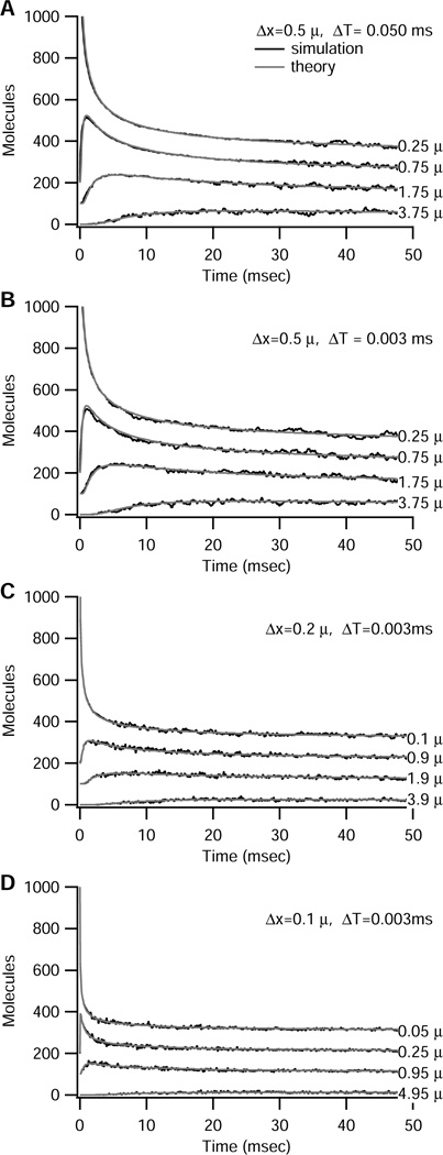
Trinomial algorithm produces results similar to that predicted by theoretical deterministic solution, independent of time step ΔT and compartment size Δx. Initial number of molecules = 1000 in left-most compartment (center is 0.25 µm from end) of 10 µm long structure. Results for different compartments are offset by 100 for illustration purposes. For all panels, gray lines show the theoretical solution; black lines show simulations. The algorithm seamlessly switches from deterministic to stochastic equations when the molecules in a compartment drops below 100. (A) Δx = 0.5 µm, ΔT = 0.05 ms, (B) Δx = 0.5 µm, ΔT = 0.003 ms, (C) Δx = 0.2 µm, ΔT = 0.003 ms, (D) Δx = 0.1 µm, ΔT = 0.003 ms.

To further assess the algorithm for small numbers of molecules, the left most compartment is initialized with 100 molecules (Δx = 0.05 µm and ΔT = 0.025 ms); thus the deterministic equations are never used for these solutions. The number of molecules in compartment 0.25 µm (Fig 3A), 1.75 µm, (Fig 3B) and 5.75 µm (Fig 3C) are illustrated for three different trials each to further demonstrates the natural variation of the stochastic algorithm. Notice that the number of molecules fluctuates considerably about the theoretical deterministic solution, though averaging over multiple trials decreases the fluctuations and yields a trajectory closer to the theoretical (results not shown). Though the theoretical solution reaches the steady state value of 5 molecules per compartment within 200–300 ms, the stochastic solution continues to fluctuate; thus steady state is reached only on average. The actual fluctuations may be larger than illustrated because the solution in this and other figures is plotted at a 0.1 ms resolution.

Figure 3.

With small numbers of molecules, the trinomial algorithm solution has the same dynamics as the deterministic theoretical solution, though the fluctuations in number of molecules are considerable. Initial number of molecules = 100 in left-most compartment (center is 0.25 µm from end) of 10 µm long structure. Three different trials are overplotted with the theoretical solution for compartments with centers at (B) 0.25 µm, (C) 2.25 µm, and (D) 6.25 µm. Note different scales in each graph.

The binomial version of the algorithm is more general because it may be used for both two- and three-dimensional diffusion. To illustrate the accuracy of this algorithm in the two-dimensional case, a 10 µm × 10 µm structure is subdivided into 400 0.5 µm² compartments. The corner compartment (at 0.25 µm,0.25 µm) is initialized with 1000 molecules at time 0; thus both deterministic and stochastic algorithms are utilized. The theoretical, steady state solution for two-dimensional diffusion in a semi-infinite sheet is 2.5 molecules per compartment; thus, comparison of the stochastic solution with the theoretical solution is valid only for time < 100 ms. Simulations results are portrayed in Figure 4 using both ΔT= 0.05 ms and ΔT= 0.013 ms time step. Fig 4A illustrates the solution for four compartments along one edge; Fig 4B illustrates the solution for four compartments along the diagonal. In both cases, the theoretical solution lies within the simulated solution, but the fluctuations in the simulated solution are relatively large, especially when the number of molecules is small. Notice that the only difference between the 0.05 ms time step and the 0.013 ms time step is the fluctuations, showing the robustness of the binomial algorithm to time step.

Figure 4.

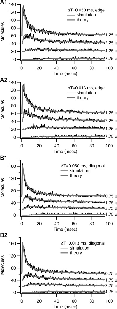
Binomial algorithm produces results similar to that predicted by theoretical solution to deterministic case. Initial number of molecules = 1000 in corner compartment (center is 0.25 µm, 0.25 µm) of 10 µm by 10 µm structure; Δx = Δy = 0.5 µm in all panels. For all panels, gray lines show the theoretical solution; black lines show simulations. Results for different compartments are offset by 20 for illustration purposes. (A) Compartments along edge (center =0.25 µm in x direction, with y distance indicated in µm to right of trace). A1 uses ΔT = 0.05 ms; A2 uses ΔT = 0.013 ms. (B) Compartments along diagonal (x distance=y distance in µm indicated to right of trace). B1 uses ΔT = 0.05 ms; B2 uses ΔT = 0.013 ms.

To demonstrate diffusion in a sheet when only the stochastic algorithm is employed, the compartment 0.25 µm,0.25 µm was initialized with only 100 molecules at time 0. In this case, the stochastic solution is comparable to the theoretical semi-infinite solution for all time because the theoretical steady state value is < 1 molecule per compartment. Fig 5A-D show three different trials in (A) compartment 0.25 µm, 0.25 µm, (B) compartment 0.25 µm,0.75 µm, and (C) compartment 1.25 µm, 1.25 µm. The number of molecules decreases very quickly with distance from the corner, and, a mere 2 µm from the corner, the theoretical solution does not exceed 2 molecules per compartment. In contrast to the theoretical solution, the simulation demonstrates considerable variation among the different trials in all compartments, and, e.g. at time = 7 ms ranges from 0 to 6 molecules when the theoretical solutions is ~2 (Fig 5C, arrow). These fluctuations are important because they can produce significant differences in the activation of downstream molecules.

Figure 5.

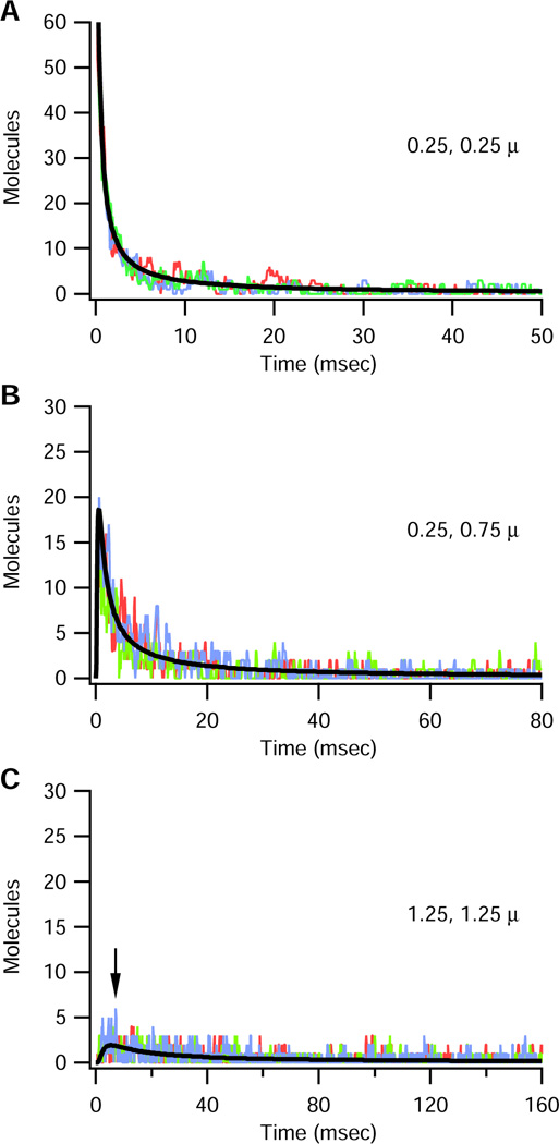
Results of binomial algorithm when 10 µm × 10µm structure is initialized with 100 molecules in corner compartment. In all panels, the smooth black line indicates theoretical solution, thin fluctuating lines show three simulation trials. An arrow points to the time when the theoretical solution is 2 molecules in the compartment, yet the simulated solution ranges between 0 and 6 depending on the trial.

These algorithms may be used to simulate diffusion within neuronal dendrites. In this case, the one dimensional trinomial algorithm is integrated with the multi-dimensional binomial algorithm to model diffusion in a spatially complicated structure. As an example, a dendritic segment is modeled as 10 µm in length by 2 µm in diameter. The dendrite is segmented into 2D rings of width 0.5 µm and length 0.5 µm, resulting in 40 circumferentially homogeneous compartments. Five spines, 0.5 µm diameter by 1.5 µm in length and segmented into 3 1D compartments of length 0.5 µm, are evenly spaced along the dendrite. For this type of simulation, additional lookup tables are created to store the connections between one dimension structures (spines) and two dimensional structures (dendrites). Also, the direction lookup tables are modified to include movement into the spine from the dendrite, which is proportional to the contact area between spine and dendrite.

Figure 6 evaluates the effect of spines and molecule source on the number of molecules in the dendrite (in the outer ring at the base of the spine). Three conditions are illustrated: (1) 2000 molecules are placed at one end of the dendritic segment (Fig 6: light gray traces); (2) 2000 molecules are placed at one end of the dendritic segment, but there are no spines (Fig 6: black traces, mostly covered by light gray traces); (3) each of the spines is initialized with 400 molecules in the spine head (Fig 6: medium gray traces). Comparison of conditions 1 and 2 evaluates whether the presence of spines modifies the number of molecules in each dendritic compartment. As observed in Fig 6, the presence of spines does not decrease the number of molecules in the dendrite compartment, either for the ring shaped compartment at 1.75 µm (close to the source, thus an initial transient elevation in molecules is seen) or the ring shaped compartment at 7.75 µm (far from the source, thus the number of molecules rises slowly to steady state). Comparison of the first and third cases illustrates how the peak number of molecules adjacent to the spine head depends on the initial source of the molecules. When molecules originate in the spine head, the number of molecules in the adjacent dendritic ring rises very quickly (within 100 ms) to its steady state value, with no overshoot. Also, the effect of distance is eliminated; thus the number of molecules is independent of spine location (though there is variation due to the stochastic algorithm). Consequently, in ring 1.75 µm, which had an initial transient elevation, the peak value is significantly smaller when molecules originate in the spine. The stochastic variation can be seen by comparing Fig 6A with 6B: the number of molecules reaches 100 within ~10 ms in ring 7.75 µm, but only reaches ~60 during the same time frame in ring 1.75 µm, and then slowly increases to steady state.

Figure 6.

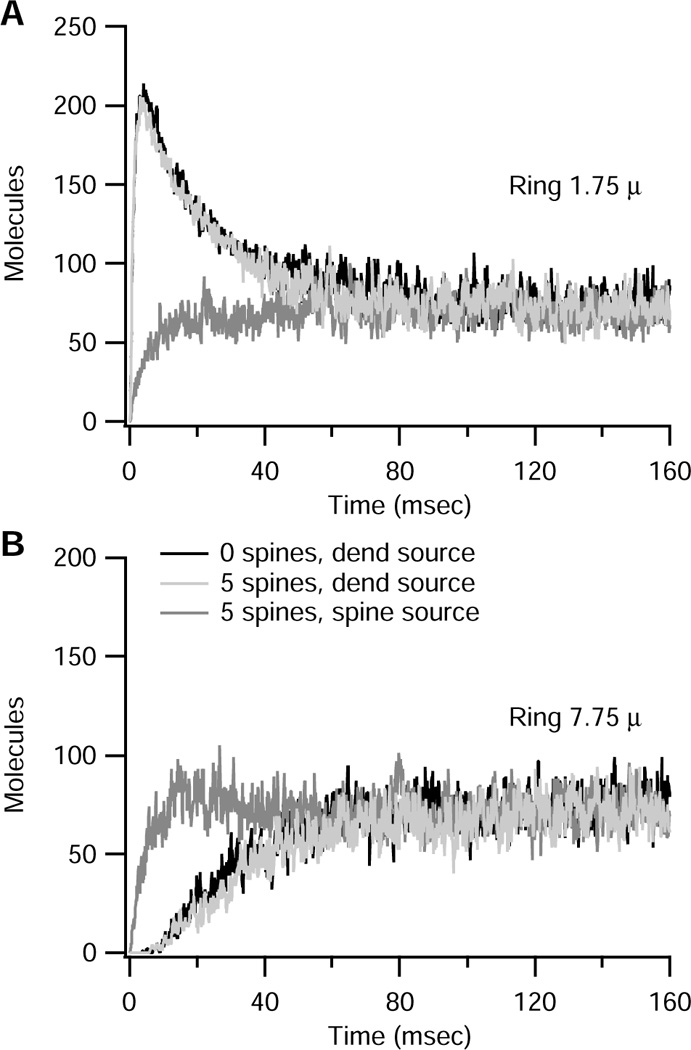
Effect of spines and molecule source on the number of molecules in a dendritic compartment at the base of a spine. (A) Ring shaped compartment located at 1.75 µm, (B) Ring shaped compartment located at 7.75 µm. Both panels compare three different conditions: (1) 2000 molecules are placed at one end of the dendritic segment (light gray traces); (2) 2000 molecules are placed at one end of the dendritic segment, but there are no spines (black traces); (3) each of the spines is initialized with 400 molecules in the spine head (medium gray traces). Light gray traces almost completely cover black traces, indicating that the presence of spines does not affect number of molecules in the dendrite, because their volume is so small. When molecules are initialized in spines, the number of molecules in the dendrite rises more uniformly and reaches its steady state value more quickly. When molecules are initialized at the end of the dendrite, a transient peak appears in the compartment close to the dendrite end, but not in the more distal compartments.

The spatio-temporal distribution of diffusion molecules is displayed in Fig 7 in a format analogous to the line scans used with calcium imaging: the abscissa indicates time and the ordinate indicates compartment. As portrayed in Fig 7E, compartment 0 is the spine head; compartments 1 and 2 are the spine neck; compartment 3 is the submembrane dendritic ring; and compartment 4 is the cylindrical inner core of the dendrite. In order to compare these different sized compartments, the concentration of molecules (calculated by dividing moles by compartment volume) is illustrated (see color scale in 7F) for the spine and adjacent dendrite located 1.75 µm from the origin (Fig 7A,B) and for the spine and adjacent dendrite located 7.75 µm from the origin (Fig 7C,D). Fig 7A,C (two different spines) illustrates that the concentration in both spines is very high (>0.3 µm) for the first 10 ms when the molecule source is the spine head. In contrast, the number of molecules in the dendrite remains low during this initial period. As the molecules diffuse out of the spine, the number of molecules in the dendrite increases, but never reaches a high concentration. This is not due to an explicit diffusional barrier, nor to buffering (not included in the simulation), but simply due to dilution of the molecules by the larger dendritic volume. Fig 7C,D illustrate the number of molecules in the same compartments when the molecules are initialized in the dendrite. In this case, the concentration in the spine reflects that in the dendrite. In the compartments at 1.75 µm, the number of molecules in both dendrite and spine compartments are transiently elevated during the first 25 ms; however, in the compartments at 7.75 µm, the number of molecules remains near zero until 40 msec. The other notable difference is that spine concentration fluctuates significantly more than the dendritic concentration. After the first 100 ms, the dendrite concentration has a coefficient of variation of 0.1, whereas the spine concentration has a coefficient of variation of 0.4 (mean concentration = 0.1 µm for both). Thus, the source of diffusing molecules has a dramatic effect on the concentration of molecules in the spine head and this will greatly affect activation of enzymes.

Figure 7.

Dendritic spines permit high local molecule concentrations. (A-D) Concentration (gray shade) vs time (x axis) and compartment (y axis). (A,B) Spine and attached dendrite 1.75 µm from end. (C,D) Spine and attached dendrite 7.75 µm from end. (A,C) Molecule source is spine head (compartment 0 of spine). (B,D) Molecule source is dendrite end (0 µm). When molecule source is spine head, the spine concentration is very high (> 0.3 µm) for the first 10 ms, yet dendrite concentration never exceeds 0.1 µm. When the molecule source is the dendrite, concentration of the proximal spine reaches 0.3 µm briefly, but concentration of the more distal spine never exceeds 0.1 µm. (E) Geometry of dendrite and attached spines. The cylinder is subdivided radially into an outer ring of 0.5 µm width and an inner core of 0.5 µm radius, and subdivided lengthwise into 0.5 µm long compartments. Spines are evenly distribut4ed along the length. The inset shows the geometry of one spine and part of attached dendrite. Numbers indicate compartments visualized in A-D. (F) Color scale used for panels A-D.

The efficiency of the algorithm is sufficient to allow simulation of second messenger pathways in a multitude of spines on the dendritic trees of an entire neuron. One application would be to investigate the effect of anchoring proteins on synaptic plasticity. Such a simulation requires both a model of the entire neuron to achieve the correct electrical activity, and the detailed second messenger pathways within spines. In addition, sufficiently small spine compartments are required to allow the anchoring proteins to be localized at the post-synaptic density. To evaluate the scalability of the algorithm for such a model, the simulations of dendrite plus spines are repeated using a longer dendrite, more spines and smaller compartments, of a size appropriate to address the function of anchoring proteins. As expected, the simulation time (table 1) scales with the number of compartments and time steps, and is still very fast for this structure. More importantly, the simulation time does not scale with the number of molecules: the simulations using 1000 molecules were only slightly longer than simulations using 100 molecules for the one dimensional structure.

Table 1.

User time on a Dell Precision 350 Workstation with 1 GB of 400 MHz (FSB) RDRAM for the simulations presented in the results. Both the number of compartments and size of each compartment is listed under “compartment”.

Simulation	Time step	compartments	User Time
1D	25 µsec	20, 0.5 µm	0.320s (1000 mol) 0.290s (100 mol)
2D Cartesian	25 µsec	400, 0.5 µm	2.25s (1000 mol) 0.63s (100 mol)
10 µm Dendrite+5 spines	25 µsec	65, 0.5 µm	1.36s (2000 mol)
20 µm Dendrite+20 spines	6.25 µsec	440, 0.25 µm	13.30s (2000 mol)

Part of the algorithm’s efficiency is in the use of uniform random numbers to lookup the number of moving molecules in a table filled with binomial or trinomial random numbers. Thus, efficiency is related to how often the table entries are re-used, and how many table entries must be searched to find the number of moving molecules. Fig 8A shows a histogram of how many entries in the trinomial distribution table are used with a particular frequency. During a simulation of 1000 molecules diffusing in a one dimensional, 10 µm long structure (20 compartments) for 1000 ms (ΔT=0.003 ms), ~7700 entries are used once or not at all, and ~1100 entries are used two or more times. Fig 8B shows a use histogram of the binomial distribution table entries for a 1000 ms simulation in a two dimensional, 10 µm × 10 µm structure (400 compartments). Only 1600 entries are used zero or one time, and the remaining 700 entries are used two ore more times. As expected, the fractional use of the table entries equals the probability of the table entry for both the binomial and the trinomial (Fig 8C). Note that not all entries are searched each time step, either for the binomial or trinomial. Each row of the table is indexed by the number of molecules in the compartment, N; thus, during each time step, only the entries corresponding to N molecules are searched. The number of entries searched is further reduced by defining a minimum probability to store in the table. For the simulations presented here, if the probability of an event is less than 1e-15, it is considered too unlikely to store; consequently, a maximum of 136 entries are searched for the trinomial, and even fewer for the binomial.

Figure 8.

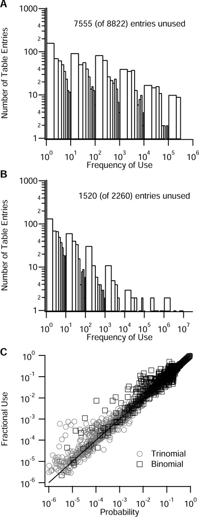
Histogram showing frequency of use of table entries during stochastic simulations. The number of unused entries, which is significant for these short simulations, decreases as the simulation time increases. Minimum probability stored = 1e-15. (A) Frequency of use of trinomial tables during 1000 ms simulation with ΔT=0.003 ms (B) Frequency of use of binomial tables during 1000 ms simulation with ΔT=0.003. (C) The frequency of use of each table entry (normalized by the total number of times a table row was used) equals the fractional probability for that table entry.

To improve the efficiency of the algorithm, the number of unused entries can be reduced by increasing the minimum probability stored. For example, when a minimum probability of 1e-9 is used for the two dimensional simulation (ΔT=0.025), the number of unused table entries decreases to 659 out of a total of 1110 table entries, without a change in the results. On the other hand, for longer simulations of larger structures, the number of unused entries will decrease without changing the minimum probability stored. For example, in a 2000 ms simulation of a 20 µm long × 2 µm diameter dendrite with 20 spines, using ΔT=25 µs, Δx=0.5 µm, and 5,000 molecules, only 1308 of the 3093 binomial table entries are unused, and more of the low probability table entries are used with a higher frequency as compared to Fig 8B.

DISCUSSION

A stochastic diffusion algorithm was derived for use in simulating second messenger pathways within neurons. Simulations in one and two dimension were compared with the theoretical solution to the deterministic diffusion equation for finite and semi-infinite structures. The solutions were found to fluctuate around the theoretical solution, thereby validating the algorithm, and also illustrating how stochastic simulations can produce results that differ from deterministic solutions. A simulation of stochastic diffusion within a dendrite with attached spines illustrated the potential of the algorithm for simulating second messenger pathways within neurons, and demonstrated that spines compartmentalize molecules by virtue of their small volume relative to the dendrite.

The computationally efficient stochastic diffusion algorithm is derived from a random walk model of diffusion by allowing multiple diffusion events to occur within a single time interval. This approach is similar to that used to derive the computationally efficient tau-leap algorithm for stochastic biochemical reactions (Gillespie, 2001), and requires the number of molecules leaving a compartment to produce a relatively small change in molecule quantities at each time step. Under these conditions, the movements of individual molecules can be considered independent, and thus binomial or trinomial probability distributions can be used to calculate the number of moving molecules. In a long thin structure, in which it is appropriate to consider one-dimensional diffusion only, a single random number determines not only the number of molecules leaving the compartment, but their direction. For two and three dimensional diffusion, after determining the number of molecules leaving the compartment, additional random numbers are required to determine the destination compartments only for the molecules leaving. Thus, the gain in speed is obtained by considering collections of molecules, instead of tracking the movement of individual molecules.

The computational efficiency of the algorithm derives from the following properties: (1) The probabilities p_m, p_f, p_b and p_n are independent of the number of particles, and depend only on the time step and compartment size, thus they can be pre-computed for each compartment. (2) The probabilities for each combination of N, k_f, k_b (or N, k_m for the binomial) are pre-computed because these equations are used only for compartments in which the number of particles is sufficiently small that deterministic algorithms are inaccurate, e.g. for N < 100. (3) A table lookup stores the pre-computed binomial or trinomial probabilities mapped to the unit number line, thus table lookup requires uniform random numbers, instead of binomial or trinomial random numbers. (4) Since most of the molecules remain in the compartment, random number generation is not required for a majority of the molecules in the simulation. In summary, the proposed algorithm is efficient because it minimizes the number and type of random numbers used.

Second messenger pathways include not only diffusion but also biochemical reactions; therefore, simulation of second messenger pathways requires that this stochastic diffusion algorithm be integrated with an equally efficient algorithm for stochastic biochemical reactions. To maintain the efficiency achieved by considering collections of molecules, it is logical to integrate the stochastic diffusion algorithm with the tau-leap algorithm (Gillespie, 2001), or one of the later modifications of the algorithm (e.g. Cao et al. 2005). The tau-leap algorithm determines the number of molecules that participate in each reaction at each time step. In the original implementation, a Poisson random number was used to determine the number of reaction events for each reaction. The non-zero probability of choosing a random number greater than the number of substrate molecules allowed molecule populations to become negative. Subsequent versions of the algorithm implemented techniques to prevent negative populations. One method is to use the exact stochastic algorithm (Cao 2005), when the number of substrate molecules is very small, e.g. below 5 or 10. Another method is to use the binomial distribution to calculate the number of reaction events for each reaction (e.g. Tian and Burrage 2004, Chatterjee et al. 2005), which limits the number of reaction events to the number of substrate molecules. The selection of the particular tau-leap algorithm to integrate with the present stochastic diffusion algorithm requires careful consideration to maintain efficiency and accuracy. An integrated algorithm would calculate the number of molecules either reacting or diffusing during each time step; and provisions would be made to ensure that the total of all reaction and diffusion events for each molecule type neither appreciably changes molecule quantities during a single time step, and nor produces negative molecule quantities.

The purpose of this integrated algorithm is to emulate the dynamics of diffusion and biochemical reactions, which are components of second messenger pathways, within the extensive and complicated geometrical structure of entire neurons. The number of molecules within neurons requires that the algorithm excludes details often included in exact stochastic simulations in order to minimize the number of calculations and the generation of random numbers. In particular, in small structures such as spines, intracellular organelles such as mitochondria and non-linear geometry may be obstacles to diffusion. An increase in the number of collisions with these structures produces a longer path length than predicted by the diffusion coefficient measured without such obstacles. Furthermore, if some of these collisions are with binding proteins, anomalous diffusion may be observed (Saxton 2001). The stochastic diffusion algorithm by itself cannot account for these effects; however, the algorithm integrated with the tau leap algorithm or other stochastic biochemical reaction algorithms can simulate reaction diffusion systems. Further investigation is required to determine if such anomalous diffusion can be modeled by including reactions with binding proteins and, if necessary, decreasing the diffusion coefficient to account for an increase in path length.

The present algorithm assumes that electrical fields are not present or that the diffusing molecules are not charged. Though this assumption may be true for electrically neutral molecules such as inositol triphosphate, it is not true for ionic species such as calcium diffusing in the electrically charged environment of excitable neurons. This assumption of electrical neutrality is implicit in most diffusion algorithms (Bhalla 2004a,b, Blackwell and Kotaleski 2002, Elf and Ehrenberg 2004, Stiles et al. 2001, Schaff 1997, Slepchenko et al. 2003), in part because biochemical reactions with other molecular species are considered to be more significant effects. Nonetheless, it may be necessary to include electric field effects in future versions of the diffusion algorithm, after it has been integrated with a stochastic biochemical reaction algorithm.

This stochastic diffusion algorithm integrated with the tau-leap algorithm presents an approach rather different than other approaches for simulating stochastic reaction-diffusion systems. One other approach uses a grid-free stochastic diffusion method, in which molecules move a random distance in a random direction. MCell (Stiles et al. 2001) is the paragon of such approaches, and achieves computational efficiency by using table lookup for distance and direction, bit-level random numbers, and ray tracing to identify possible biochemical reactions. This exact method for stochastic reaction-diffusion has been used to investigate aspects of synaptic physiology (Stiles et al. 1999). The algorithmic difference with the present approach has its source in the different objectives of the two approaches. MCell seeks to reproduce interactions at the nanoscale level, and may be used to understand e.g. how details of spine geometry influence calcium influx through synaptic channels. In contrast, the stochastic diffusion algorithm described herein is designed for mesoscopic level modeling, and may be used to understand how processes in spines influence and are influenced by ionic channels in the dendrite. Such an approach is ideal for investigating synaptic plasticity, where electrical activity will determine the level of activation of second messengers and down stream enzymes, and the phosphorylation of ionic channels by those enzymes will modulate electrical activity.

Another approach extends exact stochastic reaction algorithms, e.g. the next reaction method (Gibson and Brook, 2000) or the first reaction method (Gillespie 1977), to systems with multiple spatial compartments; thus these are grid-based approach similar to the present algorithm. In both the spatial next reaction algorithm (Elf et al. 2003, 2004) and the newest Kinetikit algorithms (Bhalla 2004a, 2004b), diffusion is treated as an additional reaction, and each “reaction event” is either reaction or diffusion. The propensity for diffusion is calculated from the diffusion coefficient divided by the squared length of the compartment, and thus is similar to equation 1, which defines the probability of a molecule leaving a compartment. Despite their differences, both of these approaches are exact and, because calculations are applied to individual molecules, scale with the number of molecules in the system. The latter characteristic is what interferes with these approaches being applied to entire neurons. On the other hand, the Kinetikit algorithm switches to a deterministic algorithm for compartments with large numbers of molecules, thus it also may be capable of simulating second messenger pathways in entire neurons.

The computationally efficient stochastic diffusion algorithm paves the way to a new class of neuronal model, one that integrates the information obtained from biochemical, pharmacological, and molecular biology experiments with the more traditional multi-compartmental models of neurons. The resulting integrative model provides insight into mechanisms underlying neuromodulatory effects and the functional consequences of neuromodulators with respect to neuronal activity. Such models will be useful for investigating questions such as the mechanism whereby lack of dopamine produces deficits in neuronal function observed in Parkinson’s Disease.

REFERENCES

- Abel T, Nguyen PV, Barad M, Deuel TA, Kandel ER, Bourtchouladze R. Genetic demonstration of a role for PKA in the late phase of LTP and in hippocampus-based long-term memory. Cell. 1997;88:615–626. doi: 10.1016/s0092-8674(00)81904-2. [DOI] [PubMed] [Google Scholar]
- Bhalla US. Signaling in small subcellular volumes. I. Stochastic and diffusion effects on individual pathways. Biophys. J. 2004a;87:733–744. doi: 10.1529/biophysj.104.040469. [DOI] [PMC free article] [PubMed] [Google Scholar]
- Bhalla US. Signaling in small subcellular volumes. II. Stochastic and diffusion effects on synaptic network properties. Biophys. J. 2004b;87:745–753. doi: 10.1529/biophysj.104.040501. [DOI] [PMC free article] [PubMed] [Google Scholar]
- Blackwell KT. Paired turbulence and light do not produce a supralinear calcium increase in Hermissenda. J. Comput. Neurosci. 2004;17:81–99. doi: 10.1023/B:JCNS.0000023866.88225.03. [DOI] [PubMed] [Google Scholar]
- Blackwell KT, Hellgren Kotaleski J. Modeling the dynamics of second messenger pathways. In: Kotter R, editor. Neuroscience Databases: A Practical Guide. Norwell, MA: Kluwer Academic Publishers; 2002. [Google Scholar]
- Cao Y, Gillespie DT, Petzold LR. Avoiding negative populations in explicit Poisson tau-leaping. J. Chemical Physics. 2005;123 doi: 10.1063/1.1992473. 054104. [DOI] [PubMed] [Google Scholar]
- Chatterjee A, Vlachos D, Katsoulakis M. Binomial distribution based tau-leap accelerated stochastic simulation. J. Chemical Physics. 2005;122 doi: 10.1063/1.1833357. 024112. [DOI] [PubMed] [Google Scholar]
- Elf J, Doncic A, Ehrenberg M. Mesocopic reaction-diffusion in intracellular signaling. Proceedings of the SPIE's First International Symposium on fluctuations and Noise. 2003;5110:114–124. [Google Scholar]
- Elf J, Ehrenberg M. Spontaneous separation of bi-stable biochemical systems into spatial domains of opposite phases. Systems Biology. 2004;1:230–236. doi: 10.1049/sb:20045021. [DOI] [PubMed] [Google Scholar]
- Fink CC, Slepchenko B, Moraru II, Watras J, Schaff JC, Loew LM. An image-based model of calcium waves in differentiated neuroblastoma cells. Biophys. J. 2000;79:163–183. doi: 10.1016/S0006-3495(00)76281-3. [DOI] [PMC free article] [PubMed] [Google Scholar]
- Gibson MA, Bruck J. Efficient exact stochastic simulation of chemical systems with many species and many channels. J Physical Chemistry A. 2000;104:1876–1889. [Google Scholar]
- Gillespie DT. Exact Stochastic Simulation of Coupled Chemical Reactions. J. Physical Chemisty. 1977;81:2340–2361. [Google Scholar]
- Gillespie DT. Approximating accelerated stochastic simulation of chemically reacting systems. J Chemical Physics. 2001;115:1716–1733. [Google Scholar]
- Haberman R. Elementary Applied Partial Differential Equations: with Fourier series and boundary value problems. 3rd Edition. New Jersey: Prentice-Hall; 1998. [Google Scholar]
- Malenka RC, Kauer JA, Perkel DJ, Mauk MD, Kelly PT, Nicoll RA, Waxham MN. An essential role for postsynaptic calmodulin and protein kinase activity in long-term potentiation. Nature. 1989;340:554–557. doi: 10.1038/340554a0. [DOI] [PubMed] [Google Scholar]
- Malinow R, Schulman H, Tsien RW. Inhibition of postsynaptic PKC or CaMKII blocks induction but not expression of LTP. Science. 1989;245:862–866. doi: 10.1126/science.2549638. [DOI] [PubMed] [Google Scholar]
- Migliore M, Messineo L, Ferrante M. Dendritic Ih selectively blocks temporal summation of unsynchronized sistal inputs in CA1 pyramidal neurons. J Comput Neurosci. 2004;16:5–13. doi: 10.1023/b:jcns.0000004837.81595.b0. [DOI] [PubMed] [Google Scholar]
- Poirazi P, Brannon T, Mel BW. Arithmetic of subthreshold synaptic summation in a model CA1 pyramidal cell. Neuron. 2003a;37:977–987. doi: 10.1016/s0896-6273(03)00148-x. [DOI] [PubMed] [Google Scholar]
- Poirazi P, Brannon T, Mel BW. Pyramidal neuron as two-layer neural network. Neuron. 2003b;37:989–999. doi: 10.1016/s0896-6273(03)00149-1. [DOI] [PubMed] [Google Scholar]
- Press WH, Teukolsky SA, Vetterling WT, Flannery BP. The Art of Scientific Computing. 2nd Edition. Cambridge: Cambridge University Press; 1992. Numerical Recipes in C. [Google Scholar]
- Rosenmund C, Carr DW, Bergeson SE, Nilaver G, Scott JD, Westbrook GL. Anchoring of protein kinase A is required for modulation of AMPA/kainate receptors on hippocampal neurons. Nature. 1994;368:853–856. doi: 10.1038/368853a0. [DOI] [PubMed] [Google Scholar]
- Saxton MJ. Anomalous subdiffusion in fluorescence photobleaching recovery: a Monte Carlo study. Biophys J. 2001;81:2226–2240. doi: 10.1016/S0006-3495(01)75870-5. [DOI] [PMC free article] [PubMed] [Google Scholar]
- Schaff J, Fink CC, Slepchenko B, Carson JH, Loew LM. A general computational framework for modeling cellular structure and function. Biophys J. 1997;73:1135–1146. doi: 10.1016/S0006-3495(97)78146-3. [DOI] [PMC free article] [PubMed] [Google Scholar]
- Slepchenko BM, Schaff JC, Macara IG, Loew LM. Quantitative Cell Biology with the Virtual Cell. Trends in Cell Biology. 2003;13:570–576. doi: 10.1016/j.tcb.2003.09.002. [DOI] [PubMed] [Google Scholar]
- Stiles JR, Bartol TM. Monte Carlo methods for simulating realistic synaptic microphysiology using MCell. In: De Schutter E, editor. Computational Neuroscience: Realistic Modeling for Experimentalists. CRC Press; 2001. pp. 87–127. [Google Scholar]
- Stiles JR, Kovyazina IV, Salpeter EE, Salpeter MM. The temperature sensitivity of miniature endplate currents is mostly governed by channel gating: evidence from optimized recordings and Monte Carlo simulations. Biophys. J. 1999;77:1177–1187. doi: 10.1016/S0006-3495(99)76969-9. [DOI] [PMC free article] [PubMed] [Google Scholar]
- Surmeier DJ, Bargas J, Hemmings HC, Jr, Nairn AC, Greengard P. Modulation of calcium currents by a D1 dopaminergic protein kinase/phosphatase cascade in rat neostriatal neurons. Neuron. 1995;14:385–397. doi: 10.1016/0896-6273(95)90294-5. [DOI] [PubMed] [Google Scholar]
- Tian T, Burrage K. Binomial leap methods for simulating stochastic chemical kinetics. J. Chemical Physics. 2004;121:10356–10364. doi: 10.1063/1.1810475. [DOI] [PubMed] [Google Scholar]
- Tsien JZ, Huerta PT, Tonegawa S. The essential role of hippocampal CA1 NMDA receptor26 dependent synaptic plasticity in spatial memory. Cell. 1996;87:1327–1338. doi: 10.1016/s0092-8674(00)81827-9. [DOI] [PubMed] [Google Scholar]
- Tuerlinckx F, Maris E, Ratcliff R, De Boeck P. A comparison of four methods for simulating the diffusion process. Behav Res Methods Instrum Comput. 2001;33:443–456. doi: 10.3758/bf03195402. [DOI] [PubMed] [Google Scholar]
- Westphal RS, Anderson KA, Means AR, Wadzinski BE. A signaling complex of Ca2+- calmodulin-dependent protein kinase IV and protein phosphatase 2A. Science. 1998;280:1258–1261. doi: 10.1126/science.280.5367.1258. [DOI] [PubMed] [Google Scholar]