Sequential Anisotropic Multichannel Wiener Filtering with Rician Bias Correction Applied to 3D Regularization of DWI Data

Abstract

It has been shown that the tensor calculation is very sensitive to the presence of noise in the acquired images, yielding to very low-quality Diffusion Tensor Images (DTI) data. Recent investigations have shown that the noise present in the Diffusion Weighted Images (DWI) causes bias effects on the DTI data which cannot be corrected if the noise characteristic is not taken into account. One possible solution is to increase the minimum number of acquired measurements (which is 7) to several tens (or even several hundreds). This has the disadvantage of increasing the acquisition time by one (or two) orders of magnitude, making the process inconvenient for a clinical setting. We here proposed a turn-around procedure for which the number of acquisitions is maintained but, the DWI data are filtered prior to determining the DTI. We show a significant reduction on the DTI bias by means of a simple and fast procedure which is based on linear filtering; well-known drawbacks of such filters are circumvented by means of anisotropic neighborhoods and sequential application of the filter itself. Information of the first order probability density function of the raw data, namely, the Rice distribution, is also included. Results are shown both for synthetic and real datasets. Some error measurements are determined in the synthetic experiments, showing how the proposed scheme is able to reduce them. It is worth noting a 50% increase in the linear component for real DTI data, meaning that the bias in the DTI is considerably reduced. A novel fiber smoothness measure is defined to evaluate the resulting tractography for real DWI data. Our findings show that after filtering, fibers are considerably smoother on the average. Execution times are very low as compared to other reported approaches which allows for a real-time implementation.

1 Introduction

Regularization of Diffusion Tensor Images (DTI) is a problem of paramount importance as a prior step for finding connectivity in the brain. DTI are obtained from Diffusion Weighted Images (DWI), i.e., MR images acquired after applying gradients in different directions [2,25]. It has been shown that background noise present in DWI introduces artifacts in DTI [3]. In particular, in [15] some of this artifacts were analyzed. This work reported that the background noise present in the DWI produces an underestimation (bias) of indices of diffusion anisotropy which is not possible to correct once the DTI data are determined. This work justifies the need of filtering the DWI before any attempt at calculating the DTI data. In addition, in [4] the authors presented some interesting results showing a decrease in the trace as well as a bias in the anisotropy.

Many attempts have been reported to tackle DTI regularization; [26] makes a good classification of the existing techniques. These approaches can be summarized as follows:

• DWI regularization techniques carry out DWI filtering prior to determining the DTI. In [19] the authors choose a well-established method to perform non-linear anisotropic smoothing for each DW image independently. In particular, they used the method developed by Perona and Malik [21]. They do not incorporate dependencies among the DWI. In [18], the authors perform DWI smoothing by means of a total variation approach which can be casted as a variational technique in which a gradient descendent method has to be solved. In addition, in [4] the authors present a variational formulation to a maximum a posterior estimation for the noise-free DWI, using a Rician maximum likelihood term and a prior smoothing term. This is performed independently for each DWI.

• For DTI estimation methods, a simultaneous regularization and estimation of DTI out of the DWI is performed. In [27] the authors proposed a constrained variational framework for a direct estimation and regularization of DTI out of the complex DWI. The main drawback of this technique is that the complex DWI data are not always available but the natural envelope. A very interesting work [9] has been recently published in which the DTI data are regularized using directly the DWI data: the DTI are simultaneously estimated and regularized. In this work several models for the DWI are compared. The Rice model for the DWI gives rise to the better performance. The problem is posed as a maximum a posteriori estimation under a variational framework. In addition, the authors make use of the Riemannian approach and Log-Euclidean metrics proposed in [20]. In this approach, the space spanned by positive definite tensors is replaced by a regular and complete manifold for which null eigenvalues are at the infinity and negative values are not allowed in the corresponding tensor space. Common image processing techniques as interpolation and Gaussian smoothing can be thus performed unrestrictedly throughout this new space. The tensor is constructed by projecting points from the manifold back onto the tensor space. To our knowledge and in our opinion, this is the best approach to solve the noise problem in DTI.

• On the other hand, in DTI regularization approaches, the filtering is directly performed on the noisy DTI. Constraints of positive semi-definiteness are usually imposed. Some techniques work directly on the tensor elements [6,17,20] while others do it on the spectral tensor decomposition [22,8,7]. In [6] the authors propose a non-linear partial differential approach constrained to lie on a manifold on which the tensors are positive semi-definite. [17] poses the problem as a Bayesian estimation problem making use of a Markov Random Field and multivariate Gaussian distributions. Concerning the second approach, in [22] an energy function based on a Markovian model was used to regularized the noisy dominant eigenvector. In [8] an iterative restoration scheme for principal diffusion direction is proposed. Finally, in [7] a vector extension of the anisotropic filtering of Perona and Malik [21] is developed to smooth the tensor eigenvectors.

Most of these works are numerically intensive and do not make use of the underlying statistical distribution. The work by Basu et al. [4] is very interesting as it made use of the Rice model, but the DWI were processed independently which, as pointed out in [9] is not a good idea: “only the combination of all the DWI reveals the complex neural structure of the white matter”. So a method should model the DWI jointly and exploit the existing correlation among the DW components. The method by Filliard et al. [9] is, in our opinion, very interesting, as it has all the good ingredients. However, it does not exploit the correlation among the signals in the DWIs, as the joint probability function is built by multiplying the marginals which means the DWIs are considered as independent signals. In addition, it is computationally expensive and could not be considered as real-time: the execution time reported was 12 minutes. In this paper, we present a fast and simple method with results similar to the work by Filliard et al. to filter the DWI prior to the calculation of the DTI. It is based on a modified Wiener filter. It exploits the whole correlations among the DWIs. Drawbacks of this approach ¹ which are well known and have been comparatively highlighted elsewhere (for instance, in [7]) will be circumvented by two main ideas. First, information about the probabilistic nature of DWI data (i.e. the Rice distribution [10]) will be accounted for. Second, anisotropy in the filter will be included by means of estimating the parameters of the filter within estimation windows whose shapes are a function of the local characteristics of the data. Furthermore, the filter is applied sequentially to refine such estimates. Additional assumptions let us formulate the problem in closed-form manageable expressions. We come up with a simple and fast procedure which yields very good results both on synthetic images and on real DWI. In addition, the filter allows an important reduction of the DTI bias reported in the literature. A version of this filter dealing with scalar Magnetic Resonance signals (which does not include information of the Rice distribution of the data) has been recently published [16] and has drawn results comparable to other schemes based on the diffusion equation, at a lower computational cost. Here we extend this work in the direction indicated above.

2 Methods

2.1 Isotropic Solution

Let Y denote the observed dataset defined for a 3D grid with size S = P × Q × R. The DW dataset contains the 6 scalar volumes for the 6 diffusion gradient directions as well as the baseline data. The total number of variables in the observed dataset is 7S. This dataset will be considered as a column vector created by stacking column vectors of 7 components (the observations at every spatial position, each from every gradient used); the stack is created by visiting each voxel with some predefined order, but the order itself is irrelevant to the purposes of this paper.

The model Y = X + N is assumed, where X and N are the signal and the noise components, respectively. The filter performs the following operation ²

$$\mathbf{Z}={\mathbf{C}}_{\mathbf{X}}{\left[{\mathbf{C}}_{\mathbf{X}}+{\mathbf{C}}_{\mathbf{N}}\right]}^{-1}[\mathbf{Y}-{\eta }_{\mathbf{X}}]+{\eta }_{\mathbf{X}},$$ (1)

where η_X and C_X are the signal means and covariance matrix, respectively, and C_N is the covariance of the noise.

S is usually very large so the operation above is very involved; in addition, correlations tend to diminish for voxels sufficiently distant. An extreme case is to assume that voxels are mutually uncorrelated, both for the signal and for the noise. If this is the case, the covariance matrices C_X and C_N would be block-diagonal, i.e., only S blocks with size 7 × 7 located in the main diagonal would be non-zero. Specifically, denoting with Y(p) the vector of the 7 measurements for voxel p, with 1 ≤ p ≤ S, the covariance matrix of this vector would be C_X(p, p) + C_N(p, p), and this matrix would be the p-th block in the main diagonal of matrix C_X + C_N; it turns out that the inverse of this matrix is also block diagonal, where each block p in the main diagonal equals the inverse of matrix C_X(p, p) + C_N(p, p). This result makes equation (1) be decoupled voxelwise as

$$\mathbf{Z}\left(p\right)=\mathbf{U}\left\{{\mathbf{C}}_{\mathbf{X}}(p,p){\left[{\mathbf{C}}_{\mathbf{X}}(p,p)+{\mathbf{C}}_{\mathbf{N}}(p,p)\right]}^{-1}\left[\mathbf{Y}\right(p)-{\eta }_{\mathbf{X}}(p\left)\right]+{\eta }_{\mathbf{X}}\left(p\right)\right\}.$$ (2)

The vector function U{·} is defined for a vector variable. It sets each negative element of the input vector to zero. This is needed in order to guarantee that the solution lies in the positive hyper-quadrant of the 7-dimensional space. This correction keeps the positive property of envelopes unaltered and it allows the Stejskal-Tanner equation [25] to be solved properly, as it was the case with the original data. However, this does not insure that the estimated tensors have always positive eigenvalues. In practice, this is not a problem. We will further discuss on that in section 4. We can say that the local filter is linear, memoryless and space-variant. It is worth noting that the assumed model both for the signal and for the noise, although simplified, is still non-stationary as both mean vectors and covariance matrices are functions of the voxel position p. To assume that the signal is stationary is far too restrictive, but this assumption is reasonable for the noise. Accepting this, we can drop index p from the noise covariance matrix, yielding ³

$$\mathbf{Z}\left(p\right)=\mathbf{U}\left\{{\mathbf{C}}_{\mathbf{X}}\left(p\right){\left[{\mathbf{C}}_{\mathbf{X}}\left(p\right)+{\mathbf{C}}_{\mathbf{N}}\right]}^{-1}\left[\mathbf{Y}\right(p)-{\eta }_{\mathbf{X}}(p\left)\right]+{\eta }_{\mathbf{X}}\left(p\right)\right\}.$$ (3)

In addition, as the DW images are acquired independently, the noise samples present in two such images can be assumed uncorrelated. For this reason we will assume the noise covariance matrix C_N diagonal. We have to consider only 7 noise variances ${\sigma }_N^2\left(k\right)$ with 0 ≤ k ≤ 6. The number of unknowns to estimate has been considerably reduced; this number is equal to 35S + 7: 7S signal means, 28S signal covariance parameters ⁴, and 7 noise variances. If these parameters were known, equation (3) would give the local Wiener solution; however, and generally speaking, this is not usually the case so we have to find out how to estimate these parameters in advance from the observation Y.

We can rely on some assumption about the signal X. Though we said that this signal is clearly non-stationary, it is reasonable to assume that the local variation of both the means and the autocovariance matrices within a given neighborhood is less than the global variation, i.e., we will assume that the signal has only local interactions [5]. Our assumption is that the signal can be considered locally ergodic so as to use spatial averages to estimate the unknown parameters.

Let ∂(p) denote a set of L neighbors corresponding to the site (voxel) p. The set ∂(p) also includes the voxel p. We will bear in mind neighborhoods of L = ∣∂(p)∣ = 27 voxels.

We can use those neighborhoods ∂(p) to estimate the 35S + 7 unknowns. As the neighborhoods are isotropic this filter will be referred to as isotropic Wiener. This is the first approach we will present. Later on we will introduce an anisotropic counterpart.

Assuming local ergodicity in the set ∂(p) for site p, we get estimates

$${\eta }_{\mathbf{X}}\left(p\right)={\eta }_{\mathbf{Y}}\left(p\right)\approx \overline{\mathbf{Y}}\left(p\right)=\frac{1}{\mid \partial \left(p\right)\mid }\sum _{p^{\prime }\in \partial \left(p\right)}\mathbf{Y}\left(p^{\prime }\right)$$ (4)

$${\mathbf{C}}_{\mathbf{X}}\left(p\right)\approx {\mathbf{C}}_{\mathbf{Y}}\left(p\right)\approx \overline{{\mathbf{C}}_{\mathbf{Y}}}\left(p\right)=\frac{1}{\mid \partial \left(p\right)\mid -1}\sum _{p^{\prime }\in \partial \left(p\right)}\left(\mathbf{Y}\left(p^{\prime }\right)-\overline{\mathbf{Y}}\left(p^{\prime }\right)\right){\left(\mathbf{Y}\left(p^{\prime }\right)-\overline{\mathbf{Y}}\left(p^{\prime }\right)\right)}^T.$$ (5)

The estimation of the noise variances ${\sigma }_N^2\left(k\right)$, for 0 ≤ k ≤ 6, is more involved and will have a great influence in the filter output as we will see later. The problem is due to the fact that the autocovariance matrices add up as C_Y(p) = C_X(p) + C_N. One possible solution is to look for a region in the image grid for which the signal components are a priori known to be zero. In this case C_X(p) will be zero and we will have that ${\sigma }_N^2\left(k\right)$ will be equal to the element (k, k) of the autocovariance matrix C_Y(p) in that region. Thus, the sample variances in that region would give us a reasonable estimation of the noise variances. Nevertheless, that piece of knowledge may not be available or it would require the user’s supervision. The proposed solution is to introduce a free parameter λ ranging in the interval (0, 1) that will be hereafter referred to as regularization parameter which would allow us to fine tune the amount of regularization required by means of a selection of the noise variances between two given bounds as

$$\overline{{\sigma }_N^2}\left(k\right)=(1-\lambda )\overline{{\sigma }_{\min }^2}\left(k\right)+\lambda \overline{{\sigma }_{\mathit{ave}}^2}\left(k\right),$$ (6)

where $\overline{{\sigma }_{\min }^2}\left(k\right)$ is the (k, k) element of the the autocovariance matrix $\overline{{\mathbf{C}}_{\mathbf{Y}}}\left(p^{\prime }\right)$ with

$$p^{\prime }=\arg \underset{1\le p\le S}{\min }\mathrm{TR}\left[\overline{{\mathbf{C}}_{\mathbf{Y}}}\left(p\right)\right],$$ (7)

where TR[·] stands for the matrix trace and $\overline{{\sigma }_{\mathrm{a}\mathit{ve}}^2}\left(k\right)$ is the (k, k) element of

$$\frac{1}{S}\sum _{p=1}^S\overline{{\mathbf{C}}_{\mathbf{Y}}}\left(p\right).$$ (8)

We can say the higher the λ value, the higher the noise variances $\overline{{\sigma }_N^2}\left(k\right)$ and, consequently, the higher the regularization and vice versa. This parameter may be either manually set or learned by training for a specific target application. Consequently, in equation (3) we can replace the parameters by their corresponding estimates giving rise to

$$\mathbf{Z}\left(p\right)\approx \overline{{\mathbf{C}}_{\mathbf{Y}}}\left(p\right){\left[\overline{{\mathbf{C}}_{\mathbf{Y}}}\left(p\right)+\overline{{\mathbf{C}}_{\mathbf{N}}}\right]}^{-1}\left[\mathbf{Y}\right(p)-\overline{\mathbf{Y}}(p\left)\right]+\overline{\mathbf{Y}}\left(p\right),$$ (9)

where $\overline{{\mathbf{C}}_{\mathbf{N}}}$ is a diagonal matrix whose diagonal elements are the noise variance estimates $\overline{{\sigma }_N^2}\left(k\right)$.

Equations (4), (5) and (6) are coarse approximations, thus a direct implementation of equation (9) will lead to poor results, therefore, we propose here a sequential scheme [13], as follows

$${\mathbf{Y}}^{(n+1)}\left(p\right)={\overline{{\mathbf{C}}_{\mathbf{Y}}}}^{\left(n\right)}\left(p\right){\left[{\overline{{\mathbf{C}}_{\mathbf{Y}}}}^{\left(n\right)}\left(p\right)+{\overline{{\mathbf{C}}_{\mathbf{N}}}}^{\left(n\right)}\right]}^{-1}\left[{\mathbf{Y}}^{\left(n\right)}\right(p)-{\overline{\mathbf{Y}}}^{\left(n\right)}(p\left)\right]+{\overline{\mathbf{Y}}}^{\left(n\right)}\left(p\right),$$ (10)

with the initial condition

$${\mathbf{Y}}^{\left(0\right)}\left(p\right)=\mathbf{Y}\left(p\right).$$ (11)

The estimates are recalculated at iteration (n) using equations (4), (5) and (6) with the data Y⁽ⁿ⁾(p). A number of iterations N ∈ (5, 10) has been considered in the experiments as sufficient. The final solution is then given by

$$\mathbf{Z}\left(p\right)\approx {\mathbf{Y}}^{\left(N\right)}\left(p\right).$$ (12)

This will also provide local coherence among neighboring voxels, a fact that palliates the (somewhat restrictive) assumption of uncorrelation within the signal components, i.e., the sequential approach is close to a non-sequential version in which the voxels are assumed to be correlated.

2.2 Anisotropic Solution

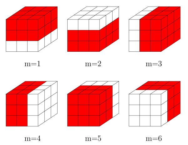
The Wiener filter introduced so far can be consider as isotropic. Hereafter we will describe how we can modify the estimation proposed in equations (4), (5) and (6) to be considered as anisotropic. This approach will be referred to as anisotropic Wiener. In figure 1 we can see six different non-homogeneous neighborhood subsystems ∂_m(p), with 1 ≤ m ≤ 6, for which a specific orientation is assumed. We can repeat equations (4) and (5) for each voxel and each orientation m using the subsystem ∂_m(p) to obtain oriented means

$$\overline{{\mathbf{Y}}^m}\left(p\right)=\frac{1}{\mid {\partial }_m\left(p\right)\mid }\sum _{p^{\prime }\in {\partial }_m\left(p\right)}\mathbf{Y}\left(p^{\prime }\right)$$ (13)

and oriented autocovariance matrices

$$\overline{{\mathbf{C}}_{\mathbf{Y}}^m}\left(p\right)=\frac{1}{\mid {\partial }_m\left(p\right)\mid -1}\sum _{p^{\prime }\in {\partial }_m\left(p\right)}\left(\mathbf{Y}\left(p^{\prime }\right)-\overline{{\mathbf{Y}}^m}\left(p^{\prime }\right)\right){\left(\mathbf{Y}\left(p^{\prime }\right)-\overline{{\mathbf{Y}}^m}\left(p^{\prime }\right)\right)}^T.$$ (14)

Then the true orientation q(p) can be estimated as

$$q\left(p\right)\approx \arg \underset{1\le m\le 6}{\min }\mathrm{TR}\left[\overline{{\mathbf{C}}_{\mathbf{Y}}^m}\left(p\right)\right].$$ (15)

The final estimation for η_X(p) = η_Y(p) and C_X(p) ≈ C_Y(p) can be determined by using equations (13) and (14) with m = q(p) for each position p, respectively. Thus, we write

$${\eta }_{\mathbf{X}}\left(p\right)={\eta }_Y\left(p\right)\approx \overline{{\mathbf{Y}}^{q\left(p\right)}}\left(p\right)\text{and}{\mathbf{C}}_{\mathbf{X}}\left(p\right)\approx {\mathbf{C}}_{\mathbf{Y}}\left(p\right)\approx \overline{{\mathbf{C}}_{\mathbf{Y}}^{q\left(p\right)}}\left(p\right).$$ (16)

Then, equation (6) can be used to estimate the noise variances $\overline{{\sigma }_N^2}\left(k\right)$ as explained before. We also propose to implement a sequential version of the anisotropic filter using the new anisotropic parameter estimation method by using equations (10), (11) and (12) as explained in section 2.1.

Fig. 1.

Oriented neighborhood subsystems with L = 27 encoding 6 different orientations (red sites).

2.3 Non-Gaussian Corrections: Inclusion of the Rice Distribution

As it is well-known, the Wiener filter, as explained along previous sections, only makes use of first and second order statistics, since this is the only information used by the linear minimum MSE estimator. As shown in appendix B, the noise-free natural envelope s of the signal (equation (B.6)) is very far from the expected value of the noisy natural envelope (equation (B.9)) for low signal to noise ratios. This will introduce a bias in the filtering procedure, since the solution is always centered about the signal mean as pointed out by equation (3). We need to estimate the Rice parameter s in order to compensate for the bias. However the noise parameter σ is also unknown. Maximum likelihood of both parameters is possible, but no closed form solution for it exists [24]. An iterative algorithm is needed, but it would be computationally very expensive. It will not give rise to a fast implementation. We have resorted the estimation problem to a simple and fast solution which follows ⁵.

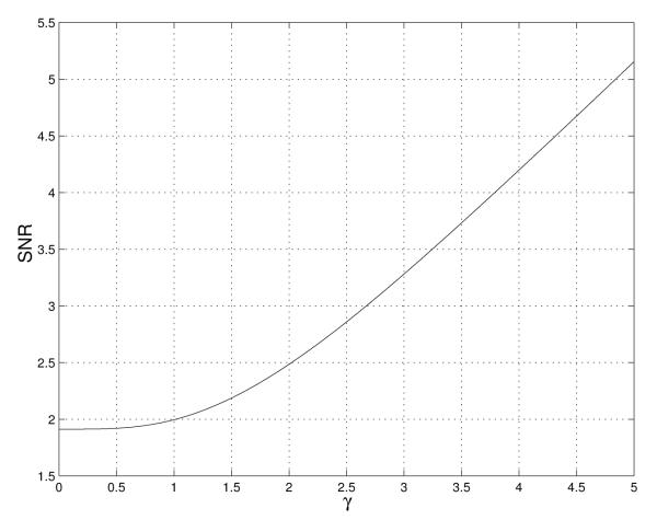
The bias effect has to be considered mainly for low SNR. For high SNR, as the Rice distribution approaches a Gaussian distribution, the Wiener solution is the general optimum solution with no bias. In figure 2 we can see the SNR as a function of the coherent to non-coherent ratio, i.e., the γ parameter. We referred to this function as B(γ) function. See appendix B for its derivation.

Fig. 2.

SNR as a function of the γ parameter.

The SNR can be estimated by the method of moments as

$$\mathrm{SNR}\approx \overline{\mathrm{SNR}}=\frac{\overline{Y}}{\sqrt{\overline{Y^2}-{\overline{Y}}^2}}.$$ (17)

From figure 2 it is clear that the B(·) function is a monotonic function of γ, thus the inverse function B⁻¹(·) is well-defined. We can write

$$\gamma =B^{-1}\left(\mathrm{SNR}\right).$$ (18)

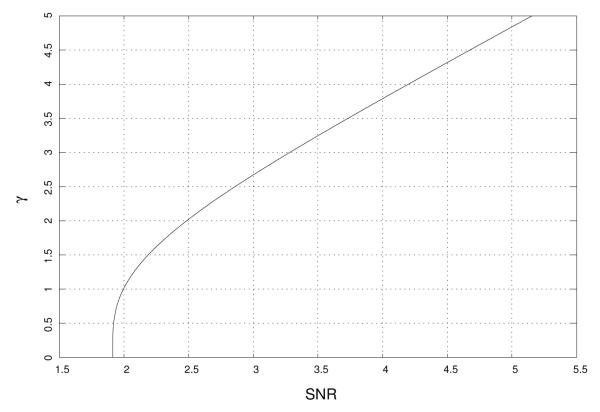
This inverse function is shown in figure 3. An estimate of the γ parameter can be determined by replacing the SNR value by its estimate given by equation (17). We can write then

$$\gamma \approx \overline{\gamma }=\{\begin{array}{cc}{B}^{-1}\left(\overline{\mathrm{SNR}}\right)\hfill & \overline{\mathrm{SNR}}>\sqrt{\frac{\pi }{4-\pi }}\hfill \\ 0\hfill & \text{otherwise}.\hfill \end{array}\phantom{\}}$$ (19)

We can write the mean-squared value using γ as

$$E\left\{Y^2\right\}=s^2\frac{2+{\gamma }^2}{{\gamma }^2},\text{therefore}s=\sqrt{\frac{E\left\{Y^2\right\}{\gamma }^2}{2+{\gamma }^2}}.$$ (20)

Finally, by replacing the parameters by their estimates we can write

$$\overline{s}=\sqrt{\frac{\overline{Y^2}{\overline{\gamma }}^2}{2+{\overline{\gamma }}^2}}.$$ (21)

The bias correction is performed by means of

$$Y^{\prime }\left(p\right)=\{\begin{array}{cc}Y\left(p\right)-\overline{Y}\left(p\right)+\overline{s}\hfill & Y\left(p\right)-\overline{Y}\left(p\right)+\overline{s}>0\hfill \\ 0\hfill & \text{otherwise}.\hfill \end{array}\phantom{\}}$$ (22)

for each voxel p. This is done independently for each of the 7 DW images. Equation (22) constrains the output to be positive, as an envelope cannot be negative. Negative values for the DWI are not possible as a logarithm is used to calculate the DTI (see for instance equation (6) in [28]). After this bias correction step, the procedures defined in sections 2.1 and 2.2 will be applied to the modified dataset. These methods are also constrained to be within the positive hyper-quadrant in the 7-dimensional space. In conclusion, no negative values are permitted so that the DTI data can be computed without difficulties as it was the case for the original data. However, in principle this does not guarantee the positive-semidefiniteness property in the estimated tensors (see section 4). However, the smoothing introduced with the use of the neighboring information improves the quality of the estimation as it will be shown in the experiments.

Fig. 3.

γ parameter as a function of the SNR.

2.4 Synthetic Data

We have created three 50 × 50 × 50 DT synthetic images with different shapes (namely, EARTH, LOGARITHM and CROSS data sets, see appendix C for a description about how these tensor data sets have been created) to evaluate the performance of the framework proposed. The associated eigenvalues for the EARTH and LOGARITHM were (λ₁, λ₂, λ₃) = (7, 2, 1). The final tensor field was normalized by 10⁻⁴. Using a value of b = 1000 and the six gradient directions (1, 1, 0), (0, 1, 1), (1, 0, 1), (0, 1, −1), (−1, 1, 0) and (−1, 0, 1) the tensor field was converted to DWI data, using as baseline the trace of the tensors. Rice noise with SNR = 10 was added to form the noisy dataset. Finally, the noisy tensor field was determined. The stochastic fiber tracking method (the random walk algorithm) proposed in [11] was used.

The CROSS synthetic data have a crossing region where two orthogonal fibers cross. This region have planar anisotropy. This example was selected to show that the filter is able to regularize regions with uncertainty. Algorithms filtering only the principal direction diffusion will fail in this case. The stochastic fiber tracking algorithm should be able to follow both paths in a smooth manner. The EARTH example was chosen to see whether a tensor field with a high variation in orientation is properly filtered. In addition, in this example the boundaries among the regions are not straight and allows to test whether the anisotropic part of the filter works properly, even though the anisotropic parameter estimation uses the simple boundaries shown in figure 1. Finally, the LOGARITHM example was selected to measure the averaged change in the anisotropy (bias correction). It is a tensor field having only prolate tensors allowing some orientation variation.

We define different measures to evaluate the performance of the filters. The DWI filtering error ∊ can be defined as

$$∊=\mathbf{Z}-\mathbf{X}.$$ (23)

The squared bias of the error is defined by

$$\mathrm{Bsq}=\frac{1}{49S^2}{\left(\sum _{k=1}^7\sum _{p=1}^S{∊}_k\left(p\right)\right)}^2,$$ (24)

where ∊_k(p) is the error at p-th voxel (out of S) in the k-th acquisition image (out of 7). The mean-squared error and the variance are defined by

$$\mathrm{MSE}=\frac{1}{7S}\sum _{k=1}^7\sum _{p=1}^S{∊}_k{\left(p\right)}^2\text{and}\mathrm{Var}=\mathrm{MSE}-\mathrm{Bsq}.$$ (25)

In order to take into account the data variability, M noisy samples under the same scenario have been generated. We can then calculate statistics at each voxel position for the DTI data. Specifically, we define the total variance TV(p) of a diffusion tensor D(p) at voxel position p, with 1 ≤ p ≤ S, as

$$\mathrm{TV}\left(p\right)=\mathrm{TR}\left[{\mathbf{C}}_{\mathbf{D}}\right(p\left)\right],$$ (26)

where for each voxel p, C_D(p) is the covariance matrix of the components of tensor D(p) as

$${\mathbf{C}}_{\mathbf{D}}\left(p\right)=E\left\{{\mathbf{D}}_V\right(p\left){\mathbf{D}}_V{\left(p\right)}^T\right\}-E\left\{{\mathbf{D}}_V\right(p\left)\right\}E{\left\{{\mathbf{D}}_V\right(p\left)\right\}}^T$$ (27)

and D_V(p) is a column vector consisting of the six different elements of the symmetric tensor D(p) arranged in any predefined order.

In equation (27), the expectations are replaced by sample means using the M available samples per voxel. In this case the sample total variance $\overline{\mathrm{TV}}\left(p\right)$ will be given by

$$\overline{\mathrm{TV}}\left(p\right)=\mathrm{TR}\left\{\overline{{\mathbf{C}}_{\mathbf{D}}}\right(p\left)\right\},$$ (28)

where for each voxel p, $\overline{{\mathbf{C}}_{\mathbf{D}}}\left(p\right)$ is the sample covariance matrix defined as

$$\overline{{\mathbf{C}}_{\mathbf{D}}}\left(p\right)=\frac{1}{M}\sum _{m=1}^M{\mathbf{D}}_V^{\left(m\right)}\left(p\right){\mathbf{D}}_V^{\left(m\right)}{\left(p\right)}^T-\frac{1}{M^2}\left(\sum _{m=1}^M{\mathbf{D}}_V^{\left(m\right)}\left(p\right)\right)\left(\sum _{m=1}^M{\mathbf{D}}_V^{\left(m\right)}{\left(p\right)}^T\right),$$ (29)

and ${\mathbf{D}}_V^{\left(m\right)}\left(p\right)$ is the m-th sample of a column vector arrangement for sample tensor D^(m)(p).

In addition to previous measures, [1,14] propose an interesting measure to quantify DTI uncertainty due to noise. They propose a new glyph representation referred to as “cone of uncertainty”, i.e., a cone whose cone angle is equal to the uncertainty (i.e., a given confidence interval) in the estimate of the orientation of the principal eigenvector and with a long axis that coincides with the mean eigenvector. We follow this idea to estimate the uncertainty.

In order to measure the confidence interval (uncertainty), we have simulated M noisy data sets. Let assume ${\mathbf{v}}_1^{\left(m\right)}\left(p\right)$ is the eigenvector associated to the largest eigenvalue for the m-th sample tensor D^(m)(p) at voxel position p. Let v₁(p) denote this same vector but of the ground truth tensor T(p) at voxel position p. The angle between these two vectors is given by

$${\alpha }^{\left(m\right)}=\text{arccos}(\mid {\mathbf{v}}_1^{\left(m\right)}{\left(p\right)}^T{\mathbf{v}}_1(p)\mid ).$$ (30)

In this expression the modulus allows to account for the problem of antipodal symmetry, i.e., eigenvectors are only defined up to its orientation along a particular axis. The closer to zero the α value the lower the uncertainty. Since in this case, equation (30) is always greater than zero, the distribution of α is necessarily one-sided. Hence, the value of α^(m) at the 0.95M-th position in the list of M samples (sorted in ascending order) constitutes the upper bound of the 95% confidence interval (CI) of the angles, i.e., the uncertainty.

In addition to this measurements, and to measure the anisotropy, we use the Fractional Anisotropy (FA) value as well as the linear, planar and spherical components as defined in [28]. With respect to the orientation, it is color coded. ⁶ We use elliptic glyphs to represent some of the results. ⁷

In addition to that, and to show the anisotropic performance of the filter, we have added an additional experiment comparing the isotropic solution with the anisotropic one. We have simulated a new synthetic data set as explained above with two clear discontinuities having only prolate tensors with orthogonal orientations.

2.5 Real Imaging Data

A DWI volume dataset using single-shot spin Echo Planar Imaging (EPI) sequence with diffusion-tensor encoding using 6 directions (1, 1, 0), (0, 1, 1), (1, 0, 1), (0, 1, −1), (1, −1, 0) and (−1, 0, 1), size 128 × 128 × 54 and voxel size 1.86 × 1.86 × 2.0mm was acquired. The non-biased anisotropic Wiener filter was run sequentially with N = 5 iterations and λ = 0.5. DTI datasets were determined both for the observed data and for the resulting data. Anisotropy and orientation are determined out of the tensor field. Additionally, we show a glyph representation for three manually-selected regions of interest. In order to quantify the bias correction in the DTI, we have segmented for each region of interest the sites corresponding to left-right (red), anterior-posterior (green) and inferior-superior (blue) by thresholding the corresponding channel in the RBG color giving rise to 9 subregions: three new regions within each manually-selected region of interest. Then, we have determined the averaged linear component, as defined in [28], in each subregion before and after filtering.

Finally, the stochastic method proposed in [11] has been applied to determine the fiber tracts. A quantitative measure μ of the smoothness along fibers has been calculated as explained in appendix D. This parameter was defined so that the lower the μ value, the smoother the fiber. An averaged smoothness $\overline{\mu }$ is defined for a set of fibers.

3 Results

3.1 Synthetic data

One noise-free synthetic tensor data set was generated for the EARTH, LOGARITHM and CROSS cases. Tractographies for the three noise-free synthetic data sets are shown in figure 4. In particular, figure 4(a) shows a tractography for the noise-free EARTH data set, figure 4(b) for the LOGARITHM and figure 4(c) for the CROSS.

Fig. 4.

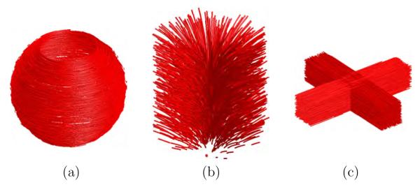
Tractography for the synthetic images: (a) EARTH, (b) LOGARITHM and (c) CROSS.

We have evaluated both the biased version of the filter (the one filtering on data Y) and the non-biased version (the one that filters the data Y’ —see equation (22)) for each noisy DWI synthetic data set. Additionally, the parameters were estimated both on the whole neighborhood (with L = 27 neighbors) and on the oriented neighborhoods (as indicated in figure 1 and equation (15)). Squared bias (Bsq), variance (Var) and MSE for the filtered DWI data sets (see equations (24) and (25)) were calculated. Achieved results are shown in tables 1, 2, 3 and 4. These tables show results for the three synthetic examples (columns): CROSS, LOGARITHM and EARTH. Values in the tables were scaled by a factor of 10⁸ for the sake of clarity. Minimum attained values have been highlighted for each measurement and synthetic case.

Table 1.

Original data corrupted by noise: bias, variance and MSE.

MEASURE	CROSS	LOGARITHM	EARTH
Bsq	0.0309	0.1376	0.0824
Var	0.8357	3.8455	1.5228
MSE	0.8666	3.9831	1.6052

Table 2.

Results for the estimation of the s parameter with no filtering. Minimum attained values highlighted for each measurement and synthetic case.

MEASURE	CROSS	LOGARITHM	EARTH	ESTIMATOR TYPE
Bsq	0.0088	0.0028	0.0885	ISOTROPIC
Var	1.1576	4.0046	2.3811
MSE	1.1664	4.0074	2.4695
Bsq	0.0027	0.0146	0.0003	ANISOTROPIC
Var	0.8537	3.8704	1.7208
MSE	0.8564	3.8850	1.7211

Table 3.

Results after filtering for λ = 0.5 and N = 5 iterations. Minimum attained values highlighted for each measurement and synthetic case.

MEASURE	CROSS	LOGARITHM	EARTH	FILTER TYPE
Bsq	0.0311	0.1387	0.0839	ISOTROPIC
Var	0.0302	0.2288	0.1024
MSE	0.0613	0.3675	0.1863
Bsq	0.0093	0.0027	0.1038	NO-BIAS ISOTROPIC
Var	0.2778	0.2734	0.5659
MSE	0.2871	0.2762	0.6697
Bsq	0.0286	0.1321	0.0755	ANISOTROPIC
Var	0.0397	0.2055	0.0791
MSE	0.0683	0.3376	0.1546
Bsq	0.0023	0.0138	0.0001	NO-BIAS ANISOTROPIC
Var	0.0525	0.2055	0.1589
MSE	0.0548	0.2193	0.1590

Table 4.

Results after filtering for λ = 0.5 and N = 10 iterations. Minimum attained values highlighted for each measurement and synthetic case.

MEASURE	CROSS	LOGARITHM	EARTH	FILTER TYPE
Bsq	0.0314	0.1400	0.0855	ISOTROPIC
Var	0.0195	0.0943	0.0983
MSE	0.0509	0.2343	0.1838
Bsq	0.0091	0.0027	0.1162	NO-BIAS ISOTROPIC
Var	0.2342	0.1133	0.4839
MSE	0.2433	0.1160	0.6001
Bsq	0.0284	0.1322	0.0750	ANISOTROPIC
Var	0.0154	0.1046	0.0556
MSE	0.0437	0.2368	0.1307
Bsq	0.0023	0.0140	0.0001	NO-BIAS ANISOTROPIC
Var	0.0263	0.0967	0.1191
MSE	0.0286	0.1107	0.1192

Table 1 represents the values for the observed noisy data. Table 2 shows values of the estimation of the parameter s only prior to the filtering stage as explained in section 2.3. Two type of estimation schemes were used (isotropic and anisotropic) as indicated by the last column (as described in sections 2.1 and 2.2 respectively).

Table 3 shows results after applying the filter for λ = 0.5 and N = 5 iterations. Isotropic and anisotropic versions of the filter as well as with and without bias correction are presented and ordered as indicated by the last column. Table 4 gives similar results but for N = 10 iterations.

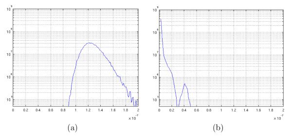
M = 100 noisy synthetic DWI data sets were computed for the LOGARITHM and the EARTH cases. Each noisy data set was then filtered. The anisotropic version of the filter with bias correction, N = 5 iterations and λ = 0.5 was selected for this experiment. The corresponding DTI data sets for the M executions were computed. The estimated total tensor variance per voxel was then determined using equations (28) and (29) for the noisy and for the filtered DTI datasets. Figure 5 shows the achieved distribution of the total variance for the different voxel positions. In particular, 5(a) shows the result for the noisy data sets and 5(b) for the filtered ones in the EARTH case.

Fig. 5.

Experimental distribution for the total variance for the EARTH data set: (a) noisy and (b) filtered.

A CI of the uncertainty angle (the angle of the “cone of uncertainty”) per voxel was determined as explained in section 2.4. Figure 6 shows the achieved distribution of the CIs for the different voxel position. In particular, 6(a) shows the result for the noisy data sets and 6(b) for the filtered ones in the LOGARITHM case.

Fig. 6.

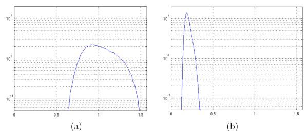
Experimental distribution for the cone of uncertainty CI for the LOGARITHM data set: (a) noisy and (b) filtered. Angles are measured in radians. The maximum allowed value is π/2.

For the total variance and the CI of the uncertainty angle, and for each case, mean and standard deviation were computed for the noisy and the filtered values. In addition, an unbalanced one-sided t-test with unknown unequal variances at a significance level of α = 0.05 was also performed to check whether or not the mean of the total variances and the mean CI of the uncertainty angle measures for the filtered valued is smaller than the noisy counterpart. Results are shown in table 5. Mean and standard deviation for the total variance was scaled by a factor of 10⁸ for the sake of clarity.

Table 5.

Statistical results for the reconstructed tensor data sets (see the main text for the details).

SYNTHETIC DATA SET	MEASURE	NOISY / FILTERED	MEAN±STD	t-TEST α = 0.05
LOGARITHM	TV×108	NOISY	30.6133 ± 3.6216	p = 0.0
		FILTERED	1.5564 ± 0.4809
	CONE CI	NOISY	1.0233 ± 0.1734	p = 0.0
		FILTERED	0.2027 ± 0.0343
EARTH	TV×108	NOISY	12.6826 ± 1.4268	p = 0.0
		FILTERED	0.3575 ± 0.3892
	CONE CI	NOISY	0.5933 ± 0.0854	p = 0.0
		FILTERED	0.1033 ± 0.0551

For illustration purposes, figure 7(a) shows the resulting tractography for the noisy CROSS data set and figure 7(b) after filtering. In figure 8 a glyph representation for a region of interest in the axial plane in the EARTH experiment is shown. Colors codify orientation. A similar representation for a coronal view in the LOGARITHM experiment is also shown in figure 8. In the three cases the anisotropic version of the proposed filtered was applied using the bias correction during N = 5 iterations and λ = 0.5. For the LOGARITHM data set, several scalar measures were determined. In table 6 the achieved results are shown for the original data, noisy data, isotropic filtering and anisotropic filtering. The filter applied the bias correction with N = 5 iterations and λ = 0.5.

Fig. 7.

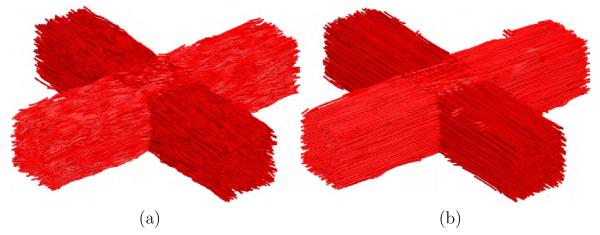
Tractography results for the CROSS synthetic image: (a) noisy and (b) filtered for λ = 0.5 and N = 5 iterations.

Fig. 8.

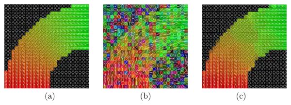
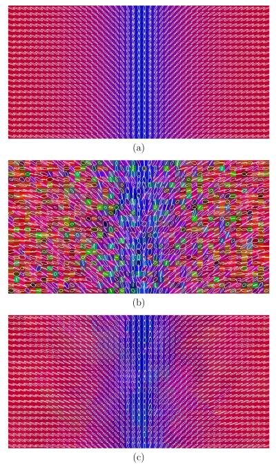
Glyph representation for the EARTH experiment. (a) original, (b) noisy and (c) filtered.

Table 6.

Anisotropy measurements for the LOGARITHM data set.

MEASURE (average)	ORIGINAL DATA	NOISY DATA	ISOTROPIC FILTERING	ANISOTROPIC FILTERING
Linear Comp.	0.7142	0.6098	0.7101	0.6933
Planar Comp.	0.1429	0.2673	0.1281	0.1551
Spherical Comp.	0.1429	0.1230	0.1618	0.1516
FA	0.7577	0.7346	0.7441	0.7424
First Eig.	7	7.5	6.9	6.8
Second Eig.	2	2.7	2.0	2.0
Third Eig.	1	0.9	1.1	1.0

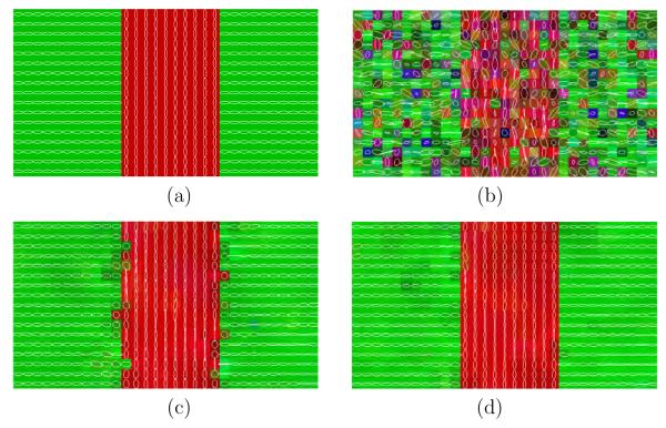
Finally, a last experiment was performed to show the need of the anisotropic filtering. In figure 10 a glyph representation with color coding orientation is shown for the original data, the noisy data, isotropic filtering and anisotropic filtering.

Fig. 10.

Glyph representation for the last synthetic experiment. (a) original, (b) noisy, (c) isotropic filtered and (d) anisotropic filtered.

3.2 Real Data

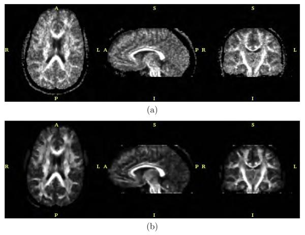
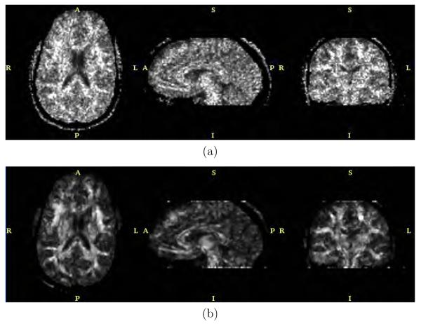
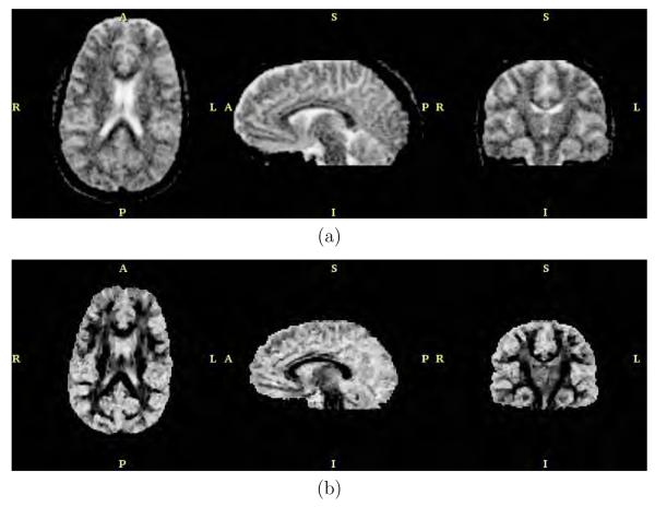
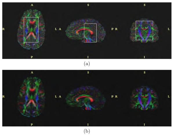
The anisotropic version of the filter with bias correction and for N = 5 and λ = 0.5 was applied to the real data. Results are shown in figures 11, 12, 13 and 14. These figures represent axial, sagittal and coronal slices for different measures of anisotropy and orientation. In particular, figure 11 shows the FA value, figure 12 the planar component, figure 13 the spherical component and figure 14 a color representation for the main orientation. In each case, the original data set and the result after filtering are shown.

Fig. 11.

FA value for the (a) original dataset and (b) after filtering.

Fig. 12.

Planar component for the (a) original dataset and (b) after filtering.

Fig. 13.

Spherical component for the (a) original dataset and (b) after filtering.

Fig. 14.

Color representation of the orientation for the (a) original dataset and (b) after filtering.

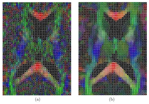
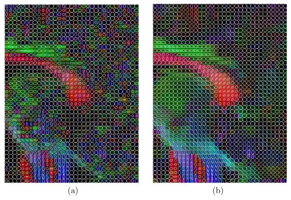
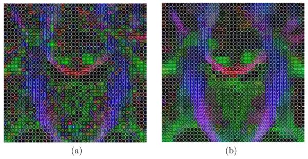
Additionally, in figures 15, 16 and 17, a glyph representation for the regions of interest highlighted in figure 14(a) is shown. In these figures colors codify orientation. As explain in section 2.5 we have determined 9 subregions by thresholding. For the sake of illustration, in figure 18 one of these subregions is shown for the original data set: the blue subregion for the coronal view. We have measured the linear component before and after regularization in these 9 subregions of interest. Results are shown in table 7.

Fig. 15.

Glyph representation for an axial region of interest. (a) original and (b) filtered.

Fig. 16.

Glyph representation for an sagittal region of interest. (a) original and (b) filtered.

Fig. 17.

Glyph representation for an coronal region of interest. (a) original and (b) filtered.

Fig. 18.

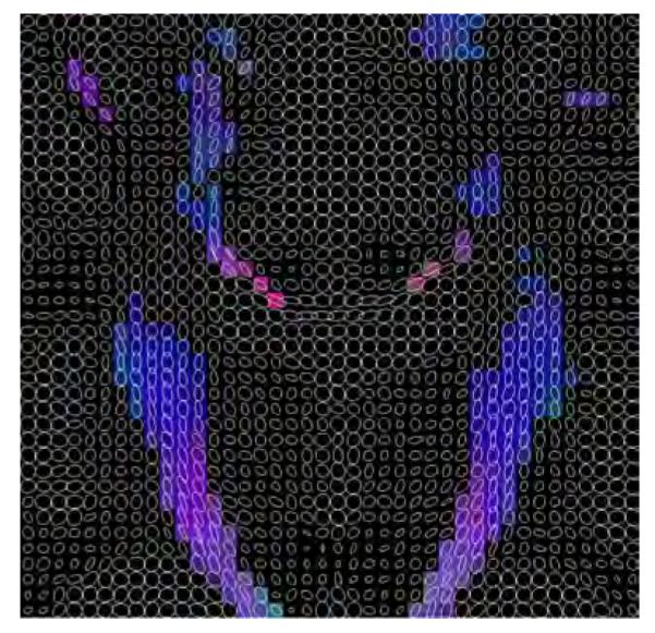
Selected areas with inferior-superior diffusion (blue areas) in the coronal view.

Table 7.

Averaged linear component in the 9 regions of interest.

ORIGINAL DATA
VIEW	LEFT-RIGHT	ANTER.-POSTER.	INFER.-SUPER.
Axial	0.5458	0.4333	0.3961
Sagittal	0.4847	0.4502	0.4634
Coronal	0.4893	0.3795	0.4318

AFTER FILTERING
VIEW	LEFT-RIGHT	ANTER.-POSTER.	INFER.-SUPER.
Axial	0.7123	0.5751	0.5386
Sagittal	0.6525	0.5932	0.6292
Coronal	0.6815	0.4800	0.5749

Finally, we have run the fiber stochastic fiber tracking algorithm for the whole brain before and after filtering. We obtained an averaged fiber smoothness $\overline{\mu }=147.6\cdot {10}^{-3}$ for the observed data and a value of $\overline{\mu }=48.1\cdot {10}^{-3}$ after applying the proposed filtering scheme.

4 Discussion

Synthetic experiments allow us to quantify how the proposed method is able to reduce the amount of noise. Tables 1, 2, 3 and 4 show some results for the DWI data sets prior to calculating the DTI. These results show how the bias is reduced by the bias correction stage and how the variance is reduced by the Wiener filtering step. In addition, as several versions of the filter were run, comparisons can be made.

Table 2 shows the result after estimating the s parameter without using the Wiener filtering. It is worth noting that low bias values were obtained at the cost of increasing variances even above the values given in table 1 for the observed data. The overall result is that the total MSE is very similar to the one given in table 1. Better results were obtained for the anisotropic estimation than for the isotropic counterpart (bold type fonts were used for the lowest values). It has to be highlighted that the LOGARITHM data set has no discontinuity. That is the reason why the isotropic and anisotropic versions of the filter give rise to very similar results for the variance and MSE (second column in table 2). However, as in the other two cases (CROSS and EARTH) some discontinuities are present, the anisotropic version of the filter gives lower values for the bias, variance and MSE.

Table 3 provides the achieved results for 5 iterations under several filter settings. When no bias correction is included, the resulting bias is similar to the one in the observed noisy data, shown in table 1. The bias correction described in section 2.3 gives rise to large reductions in the bias which are similar to those shown in table 2 but with much lower variances, resulting in low MSE values. Comparing isotropic to anisotropic filter types, and generally speaking, the anisotropic version provides lower variance, which leads to lower MSE values as well. This effect can be seen more clearly in table 4, which gives similar results but for N = 10 iterations. In this latter case, the minimum attained MSE values were obtained for the anisotropic case with bias correction for the three synthetic cases under analysis. The MSE values were 30.30, 35.98 and 13.46 times smaller than the MSE value of the noisy data for the CROSS, LOGARITHM and EARTH cases, respectively, giving rise to an average of 26.6 times smaller MSE value. It is worth noting in the LOGARITHM case, where no discontinuity is present, that the isotropic filter gives very good results and these results are very similar to the anisotropic case for this data set. In the CROSS experiment, the isotropic filter clearly fails. Though the bias is reduced from 0.0311 to 0.0093 (table 3) when the bias correction is applied, the variance increases from 0.0302 to 0.2778 (table 3) giving rise to MSE values of 0.0613 without bias correction and 0.2871 with bias correction. In conclusion, the bias correction makes the variance increase when the data set has discontinuities. With respect to the EARTH case, the situation is even worse: both the bias and the variance increase when the bias correction is included, thus making the MSE value increase from 0.1863 to 0.6697 (table 3). When the anisotropic version of the filter is considered, more reasonable results are achieved: for the three cases when the bias correction is applied the resulting bias is lower and the variance is of the same order resulting in a minimum MSE value (see tables 3 and 4).

The synthetic case also allows to evaluate the effect of the proposed method in the corresponding DTI data set. The results for the total variance and the CI of cone of uncertainty, both averaged for M = 100 repetitions, are shown in figures 5 and 6 as well as in table 5. The estimated distribution of the total variance per voxel was highly reduced as shown in figure 5 for the EARTH with a reduction of the estimated mean of the total variance by 35.47 times on the average as shown in table 5. In addition, and for the same case, the estimated standard deviation of the total variance was also reduced by a factor of 3.66 on the average. As far as the LOGARITHM case is concerned, the estimated mean of the total variance was reduced by a factor of 19.67 and the estimated standard deviation by a factor of 7.53. We can conclude that the filter makes the total variance of the DTI decrease by an average factor of 27.57 and its standard deviation by an average factor of 5.96. The t-test was passed with a very low p value (equal to zero at the numerical precision we have worked with) which leaves no room for doubt about whether the mean value was reduced thanks to the filtering.

Similar results were also obtained for the CI of the cone of uncertainty, as shown in figure 6 and table 5. The estimated mean value for the cone of uncertainty was reduced by an averaged factor of 5.4 and the estimated standard deviation by a factor of 4.1. Similarly the t-test was also passed with, say, null p-values as shown in table 5.

In figure 7 a representation for the tracts after stochastic fiber tracking is shown before and after filtering. It is clear from figure 7(b) that the tracts are smoother and that the algorithm was able to follow the two paths in the crossing region with less jumps than for the noisy data shown in figure 7(a). Figure 8 for the EARTH case allows to see how the anisotropic version of the filter with bias correction is working. The colored glyphs within the ring in figure 8(c) are of the same shape than figure 8(a): the bias effect of the Rician noise on the tensor shape (shrinking effect) has been corrected. In addition, the orientation is recovered and the regions are not mixed up due to the anisotropic nature of the filter applied, even though the boundaries are not as simple as the ones shown in figure 1 and used to estimate the parameters. To further analyze the bias correction performance of the filter in the tensor shapes, we quantify the results achieved for the LOGARITHM experiment. In this case there is no discontinuity and only one region is present, so it is possible to calculate scalar measures and average the results. In figure 8 we show the original, noisy and filtered data sets using the same glyph visualization. In this case the view is coronal. Table 6 shows the averaged values for different scalar measures for the original, noisy, isotropic filtered and anisotropic filtered data sets. In both filters the bias correction was applied. In particular, in this table we show the linear, planar and spherical components [28], the FA value and the three eigenvalues. It is clear that the Rician noise causes a shrinking effect in the tensor shapes by looking at the second column (noisy data) and comparing it with the first one (original data). The linear component has decreased its value from 0.7142 to 0.6098 and the FA value has also decreased its value from 0.7577 to 0.7346. Concerning the eigenvalues, the two larger ones have increased their values and the smaller one has decreased it. The results after filtering clearly shows how these bias effects have been properly corrected giving rise to values very close to the original ones. In this case, the difference between the isotropic and the anisotropic versions of the filter are not very significant as the LOGARITHM data set has no discontinuities.

In the last synthetic experiment, the anisotropic nature of the filter was further analyzed. To better see the results, in this experiment we have increased the amount of Rician noise in the data to levels which usually do not happen in real cases. In figure 10(c) we can see that the isotropic version of the filter clearly fails close to the boundaries: some of the tensors are wrong and the regions are clearly blurred close to the boundaries. The anisotropic version of the filter shown in figure 10(d) gives a much better result and recovers the main direction nearly perfect in all the cases. This is the reason why, though quantitative measures some times gives worse results for the anisotropic version than for the isotropic ⁸ we should always use the anisotropic version in order not to mixed up different regions.

Concerning the experiment with the real imaging case, figures 11, 12, 13 and 14 show the FA, the planar component, the spherical component and a color-coded representation of the direction of the main eigenvalue, respectively. From these figures it is clear that the amount of uncertainty within the DTI data has been considerably reduced. In particular, the background noise was fairly removed as seen for instance in the FA value in figure 11. The uncertainty of the original DTI data has a clearer effect at low FA values (isotropic areas). Figure 11(b) shows a large improvement of the FA value thanks to the variance reduction achieved by the filtering stage. Similar results could have been achieved looking at figures 12(b) and 13(b), for the planar and spherical components, respectively. The bias reduction is also an important factor which makes the mentioned figures have larger black areas, i.e., low SNR areas, which were speckled gray for the original noisy data. In our opinion the achieved enhancement for this scalar measures is outstanding. The uncertainty for the main diffusivity direction as shown in color in figure 14 was also largely reduced. A nicer appearance is achieved for the color image in figure 14(b) when compared to figure 14(a).

Figures 15, 16 and 17, for the three regions of interest shown in figure 14(a), show in detail how the filtering is working. The view is clearly smoother after filtering and both the shapes and the colors are more regular allowing better interpretation and processing of the DTI. This representation should be interpreted carefully as in each view always one of the colors cannot be represented by the glyphs as it is orthogonal to the ellipse plane. For instance, in figure 15 blue regions have circular shape as the diffusion in this case is orthogonal to the image plane. The same happens to red in figure 16 and green in figure 17. To quantify how the filter is able to cancel out the bias in the DTI (shrinking effect), in table 7 we can see the linear component [28] in the 9 segmented subregions (see section 3.2 for details about how these regions were determined). These subregions are known to have prolate tensors. In all the 9 regions the averaged linear component has improved its value after filtering. In particular, the linear component averaged in the 9 regions before filtering (averaged value of figures in table 7 top) is 0.4027 and after filtering (averaged value of figures in table 7 bottom) is 0.6041 which means that the tensors are 50% more linear in those regions after filtering.

Regarding the fiber tracking experiment, the fibers are smoother. To prove this, we can have a look at the achieved results for the fiber smoothness parameter $\overline{\mu }$ as presented in section 3.2. These results mean that after filtering, the obtained fibers were, for the defined smoothness parameter, 3 times smoother on the average.

Concerning the assumptions, as for the first order density function model used, the Rice distribution is well-known to be an appropriate model for the type of data we deal with (see for instance [10]). As for the second major assumption, i.e., the fact that data are assumed voxelwise uncorrelated, it should be pointed out that in the worst case, that is, in the presence of correlation, our design would only be a suboptimal version of a fully coupled Wiener filter. Therefore, this assumption is far from critical and does not deserve further attention. Additionally, the fact that filter parameters are estimated using data from the surroundings of each voxel under study imposes spatial coherence, as can be clearly seen from the image experiments included in the paper. The anisotropic estimation was clearly proved in the experiments which avoids blurring the boundaries. The bias correction achieved in the experiments supports the fact that the DTI data should be filtered on the DWI space and not directly on the DTI, otherwise the filter will not be able to correct for the shrinking effect which is not due to the filtering itself but to the noise.

The reader is referred to our previous paper [16] to see the effect of the λ parameter on the filtering result. In this paper, this free parameter was analyzed in depth. It concerns mainly to the noise level estimation and the degree of regularization achieved. We have compared the obtained valued of the noise covariance using λ = 0.5 for the real data set used and the value obtained using a manually segmented region without signal ⁹. The corresponding covariance matrices were of the same order of magnitude for the first iteration of the algorithm and also converged to similar values in the subsequent iterations.

With respect to the property of positive-definiteness of the DTI data, we have to highlight that our method does not impose any constraints to the DWI so as to achieved non-negative eigenvalues. For this reason, tensors with negative eigenvalues may happen. However we have seen that this is not a real problem. After filtering, all the negative eigenvalues happened to occur in the regions outside the patient were no signal is present. No significant impact on the results is thus found. As a result of the filtering process all the negative eigenvalues happening in the brain region were corrected. Imposing this constraint in the model would be a better solution, but it would make the filter more complicated, making its real-time implementation impossible.

The described results have served as a testbed for the presented DWI filtering approach. In summary, it can reduce the amount of noise and uncertainty not only for the original DWI but also for the DTI to levels similar to current state-of-the-art approaches reviewed in the introduction. These approaches are in general computationally very expensive. We here propose an alternative solution which is much more simple albeit giving rise to very acceptable results. The execution times for a compiled version of the filter in an averaged state-of-the-art machine for the real data (whose volume size was 128 × 128 × 54) were 10.3 and 30.6 seconds per iteration for the isotropic and the anisotropic versions, respectively. These figures make the filter useful for real-time applications.

5 Concluding remarks

The presented method makes proper use of the available DWI information before determining the tensors. If more gradient directions were provided, the presented method is designed to use the correlation between the signal components of the different DWI images (optimally in the mean square error sense if the parameters were known). The anisotropic approach presented for estimating the model parameters prevents the filter from mixing up data coming from different regions. Additionally, we have included in the filtering process information about the first order density function of the original data, which leads to a decrease in the bias of the filter for non Gaussian data. Results both on synthetic and on real images support the filtering methodology proposed in the paper.

Fig. 9.

Glyph representation for the LOGARITHM experiment. (a) original, (b) noisy and (c) filtered.

A Wiener Filtering Approach

We will assume the model Y = X + N, where X is the ground truth, i.e., the signal without noise, and N is the noise. Our goal is to estimate X using the observation Y. We also assume that the noise N has mean E{N} = 0 and covariance matrix C_N = E{NN^T}, which is a symmetric and positive definite matrix. With respect to the signal X we will assume a vector of means η_X = E{X} = E{Y} and covariance matrix ${\mathbf{C}}_{\mathbf{N}}=E\left\{{\mathbf{NN}}^T\right\}$, which is also symmetric and positive definite. Finally, we will assume that the signal X and the noise N are uncorrelated so E{XN^T} = 0, due to the zero-mean condition of the noise.

The Wiener filter is the optimum linear filter in the mean square error (MSE) sense, provided that the mean is known. Otherwise, more involved approaches are to be applied to guarantee the unbiased condition in the filter output [23]. Let Z denote the filter output. The linearity of the filter let us write

$$\mathbf{Z}={\mathbf{W}}^T\mathbf{Y},$$ (A.1)

where W is a coefficient matrix to be determined. The filter output is commonly constrained to be unbiased. This unbiased condition can be easily modeled by modifying equation (A.1) to

$$\mathbf{Z}={\mathbf{W}}^T[\mathbf{Y}-{\eta }_{\mathbf{X}}]+{\eta }_{\mathbf{X}}.$$ (A.2)

Needless to say, the mean has to be estimated from data, so this expression in a real-world application is only an approximation. In order to determine the coefficient matrix W, the MSE has to be minimized. The solution is well-known [12] and given by

$$\mathbf{Z}={\mathbf{C}}_{\mathbf{X}}{\left[{\mathbf{C}}_{\mathbf{X}}+{\mathbf{C}}_{\mathbf{N}}\right]}^{-1}[\mathbf{Y}-{\eta }_{\mathbf{X}}]+{\eta }_{\mathbf{X}}.$$ (A.3)

B On the SNR for Rayleigh and Rice Distributed Data

Let $Y={\tilde{Y}}_c+{\mathit{jY}}_s$ be the pre-envelope of the received signal, where Y_c and Y_s are the in-phase and quadrature components of the received signal, respectively. Due to noise during the acquisition procedure both components are independent normal variables with the same variance σ² and means s_c and s_s, respectively. This is the same as to assume the model $\tilde{Y}=\tilde{s}+\tilde{N}$ for pre-envelopes, where $\tilde{N}$ and $\tilde{s}$ are the pre-envelopes of the noise and noise-free signal components, respectively. The noise pre-envelope is $\tilde{N}=N_c+{\mathit{jN}}_s$, where N_c and N_s are the in-phase and quadrature components of the noise, respectively. Both components are independent normal variables with same variance σ² and zero means, respectively. The noise natural envelope is given by

$$N=\mid \tilde{N}\mid =\sqrt{N_c^2+N_s^2}.$$ (B.1)

It can be easily shown that this variable is Rayleigh-distribution and its probability density function is given by

$$P_N\left(n\right)=\frac{n}{{\sigma }^2}\exp \left(-\frac{n^2}{2{\sigma }^2}\right)u\left(r\right),$$ (B.2)

where u(·) is the step function. Its mean and mean-squared value are given by

$$E\left\{N\right\}=\sigma \sqrt{\frac{\pi }{2}}\text{and}E\left\{N^2\right\}=2{\sigma }^2.$$ (B.3)

Let define the signal-to-noise ratio (SNR) for a variable X as

$$\mathrm{SNR}=\frac{E\left\{X\right\}}{\sqrt{E\left\{X^2\right\}-E^2\left\{X\right\}}}.$$ (B.4)

Thus, it can be shown that for a Rayleigh variable the SNR is the constant

$$\mathrm{SNR}=\sqrt{\frac{\pi }{4-\pi }}\approx 1.913$$ (B.5)

In the absence of noise, the pre-envelope $\tilde{s}=s_c+{\mathit{js}}_s$ of the received signal has a natural envelope given by

$$s=\mid \tilde{s}\mid =\sqrt{s_c^2+s_s^2}.$$ (B.6)

The goal is to estimate this natural envelope s out of the natural envelope of the received signal $\tilde{Y}$ that can be written as

$$Y=\mid \tilde{Y}\mid =\sqrt{Y_c^2+Y_s^2}.$$ (B.7)

In this case, the this variable is Rician-distributed and its probability density function is given by

$$P_Y\left(y\right)=\frac{y}{{\sigma }^2}\exp \left(-\frac{y^2+s^2}{2{\sigma }^2}\right)I_0\left(\frac{\mathit{ys}}{{\sigma }^2}\right)u\left(y\right),$$ (B.8)

where I_n(·) is the modified Bessel function of first kind and order n. It is worth mentioning the dependence of this distribution on the noise-free component s. Inference on this component s out the observed data Y is possible in a closed manner as we will show next.

The mean of this distribution is given by

$$E\left\{Y\right\}=\sigma \sqrt{\frac{\pi }{2}}\exp \left(-\frac{s^2}{4{\sigma }^2}\right)\left[\left(1+\frac{s^2}{2{\sigma }^2}\right)I_0\left(\frac{s^2}{4{\sigma }^2}\right)+\frac{s^2}{2{\sigma }^2}{I}_1\left(\frac{s^2}{4{\sigma }^2}\right)\right]$$ (B.9)

and its mean-squared value

$$E\left\{Y^2\right\}=2{\sigma }^2+s^2.$$ (B.10)

By using equations (B.4), (B.9) and (B.10) the SNR for a Rice variable can be written as

$$\mathrm{SNR}=B\left(\gamma \right)=\frac{\sqrt{\frac{\pi }{2}}\exp \left(-\frac{{\gamma }^2}{4}\right)\left[\left(1+\frac{{\gamma }^2}{2}\right)I_0\left(\frac{{\gamma }^2}{4}\right)+\frac{{\gamma }^2}{2}{I}_1\left(\frac{{\gamma }^2}{4}\right)\right]}{\sqrt{2+{\gamma }^2-\frac{\pi }{2}\exp \left(-\frac{{\gamma }^2}{4}\right){\left[\left(1+\frac{{\gamma }^2}{2}\right)I_0\left(\frac{{\gamma }^2}{4}\right)+\frac{{\gamma }^2}{2}{I}_1\left(\frac{{\gamma }^2}{4}\right)\right]}^2}},$$ (B.11)

where γ = s/σ is known as the coherent to non-coherent ratio. In equation (B.11) the dependence of the SNR on the γ parameter was made explicit by the use of function B(·). It is worth noting that the SNR has only one degree of freedom as the dependence on the parameters s and σ is exclusively through the parameter γ. We have the following limiting values for this SNR

$$\underset{\gamma \to 0}{\lim }\mathrm{SNR}=\underset{\gamma \to 0}{\lim }B\left(\gamma \right)=\sqrt{\frac{\pi }{4-\pi }}\approx 1.913$$ (B.12)

$$\underset{\gamma \to \infty }{\lim }\mathrm{SNR}=\underset{\gamma \to \infty }{\lim }B\left(\gamma \right)=\gamma .$$ (B.13)

Equation (B.12) corresponds to the low SNR case (Rayleigh distribution) and equation (B.13) to the high SNR case (normal distribution). The bias effect has to be considered mainly for low SNR. For high SNR as the Rice distribution approaches a Gaussian distribution, the Wiener solution is the general optimum solution with no bias. In figure 2 we can see the SNR as a function of the γ parameter.

C Synthetic Tensor Data Generation

C.1 Earth

Consider the parametric family (x, y, z) = (ρ cos(θ), ρ sin(θ), α), where θ ∈ (−π, π) is the curve parameter and ρ > 0 and α are constant for each curve. Setting ρ and α and varying θ a curve is generated. The tangent vector for this curve is given by the first derivative of the curve with respect to the free parameter θ as

$$\left(\frac{\partial x}{\partial \theta },\frac{\partial y}{\partial \theta },\frac{\partial z}{\partial \theta }\right)=(-\rho \sin (\theta ),\rho \cos (\theta ),0)=(-y,x,0).$$ (C.1)

The unitary eigenvectors for the tensor field are given by

$$\{\begin{array}{c}{\mathbf{v}}_1={\left(\frac{-y}{\sqrt{x^2+y^2}},\frac{x}{\sqrt{x^2+y^2}},0\right)}^T\hfill \\ {\mathbf{v}}_2={\left(\frac{x}{\sqrt{x^2+y^2+1}},\frac{y}{\sqrt{x^2+y^2+1}},\frac{1}{\sqrt{x^2+y^2+1}}\right)}^T\hfill \\ {\mathbf{v}}_3={\left(\frac{-x}{\sqrt{x^4+y^4+x^2{y}^2+x^2+y^2}},\frac{-y}{\sqrt{x^4+y^4+x^2{y}^2+x^2+y^2}},\frac{x^2+y^2}{\sqrt{x^4+y^4+x^2{y}^2+x^2+y^2}}\right)}^T,\hfill \end{array}\phantom{\}}$$ (C.2)

where v₁ follows the tangent field given by equation (C.1). The other two eigenvectors are chosen so as to form an orthonormal set.

C.2 Logarithm

The parametric family for the curve is (x, y, z) = (ρcos(θ), ρ sin(θ), ln ρ + α), where ρ > 0 is the curve parameter and θ ∈ (−π, π) and α are constant for each curve. Setting θ and α and varying ρ a curve is generated. The tangent vector for this curve is given by the first derivative of the curve with respect to the free parameter ρ as

$$\left(\frac{\partial x}{\partial \rho },\frac{\partial y}{\partial \rho },\frac{\partial z}{\partial \rho }\right)=\left(\cos \left(\theta \right),\sin \left(\theta \right),\frac{1}{\rho }\right)=\left(\frac{x}{\rho },\frac{y}{\rho },\frac{1}{\rho }\right).$$ (C.3)

The unitary eigenvectors for the tensor field are given by

$$\{\begin{array}{c}{\mathbf{v}}_1={\left(\frac{x}{\sqrt{x^2+y^2+1}},\frac{y}{\sqrt{x^2+y^2+1}},\frac{1}{\sqrt{x^2+y^2+1}}\right)}^T\hfill \\ {\mathbf{v}}_2={\left(\frac{-y}{\sqrt{x^2+y^2}},\frac{x}{\sqrt{x^2+y^2}},0\right)}^T\hfill \\ {\mathbf{v}}_3={\left(\frac{-x}{\sqrt{x^4+y^4+x^2{y}^2+x^2+y^2}},\frac{-y}{\sqrt{x^4+y^4+x^2{y}^2+x^2+y^2}},\frac{x^2+y^2}{\sqrt{x^4+y^4+x^2{y}^2+x^2+y^2}}\right)}^T,\hfill \end{array}\phantom{\}}$$ (C.4)

where v₁ follows the tangent field given by equation (C.3). The other two eigenvectors are chosen so as to form an orthonormal set.

C.3 Cross

In this case the eigenvectors are defined by

$$\begin{array}{cc}\hfill {\mathbf{v}}_1=& \{\begin{array}{cc}{(1,0,0)}^T\hfill & \text{if}\mid y\mid <\alpha ∕2\hfill \\ {(0,1,0)}^T\hfill & \text{otherwise}\hfill \end{array}\phantom{\}}\hfill \\ \hfill {\mathbf{v}}_2=& \{\begin{array}{cc}{(0,1,0)}^T\hfill & \text{if}\mid y\mid <\alpha ∕2\hfill \\ {(1,0,0)}^T\hfill & \text{otherwise}\hfill \end{array}\phantom{\}}\hfill \\ \hfill {\mathbf{v}}_3=& {(0,0,1)}^T,\hfill \end{array}$$ (C.5)

where α is a constant representing the size of the crossing region. The corresponding eigenvalues are given by

$${\lambda }_1=\{\begin{array}{cc}7\hfill & \text{if}\mid y\mid <\alpha ∕2,\mid z\mid <\gamma ∕2\hfill \\ 7\hfill & \text{if}\mid x\mid <\alpha ∕2,\mid y\mid >\alpha ∕2,\mid z\mid <\gamma ∕2\hfill \\ 1\hfill & \text{otherwise}\hfill \end{array}\phantom{\}}$$ (C.6)

$$\begin{array}{cc}\hfill {\lambda }_2=& \{\begin{array}{cc}7\hfill & \text{if}\mid x\mid <\alpha ∕2,\mid y\mid <\alpha ∕2,\mid z\mid <\gamma ∕2\hfill \\ 2\hfill & \text{if}\mid y\mid <\alpha ∕2,\mid x\mid >\alpha ∕2,\mid z\mid <\gamma ∕2\hfill \\ 2\hfill & \text{if}\mid y\mid >\alpha ∕2,\mid x\mid <\alpha ∕2,\mid z\mid <\gamma ∕2\hfill \\ 1\hfill & \text{otherwise}\hfill \end{array}\phantom{\}}\hfill \\ \hfill {\lambda }_3=& 1,\hfill \end{array}$$ (C.7)

where γ is a constant representing the height (along the z component) of the cross.

D Smoothness along Fibers

A fiber F is given by a sorted collection of K points

$$\mathbf{F}={({\mathbf{F}}_1,\dots ,{\mathbf{F}}_k,\dots ,{\mathbf{F}}_K)}^T,$$ (D.1)

where each F_k = (x_k, y_k, z_k) is a point in the Euclidean 3D space. A collection of tangent vectors to the fiber F can be defined by taking the first difference dF as

$$\mathbf{dF}={({\mathbf{F}}_2-{\mathbf{F}}_1,\dots ,{\mathbf{F}}_{k+1}-{\mathbf{F}}_k,\dots ,{\mathbf{F}}_K-{\mathbf{F}}_{K-1})}^T,$$ (D.2)

where dF has K − 1 elements. The angle θ between two given vectors a and b is known to be

$$\theta =\text{arccos}\left(\frac{<\mathbf{a},\mathbf{b}>}{\Vert \mathbf{a}\Vert \cdot \Vert \mathbf{b}\Vert }\right),$$ (D.3)

where < ·,· > and ∥·∥ stand for the scalar product and the norm, respectively. Using matrix operations we can determine the angles θ

$$\theta ={({\theta }_1,\dots ,{\theta }_k,\dots ,{\theta }_{K-2})}^T,$$ (D.4)

spanned by adjacent tangent vectors to the fiber as

$${\theta }_k=\text{arccos}\left(\frac{{\left({\mathbf{dF}}_1{\mathbf{dF}}_2^T\right)}_{\mathit{kk}}}{\sqrt{{\left({\mathbf{dF}}_1{\mathbf{dF}}_1^T\right)}_{\mathit{kk}}{\left({\mathbf{dF}}_2{\mathbf{dF}}_2^T\right)}_{\mathit{kk}}}}\right),$$ (D.5)

for 1 ≤ k ≤ K − 2, where (·)_ij stands for the element at position (i, j) and dF₁ and dF₂ are the first K − 2 and the last K − 2 elements of dF respectively.

We define the smoothness μ for a fiber by

$$\mu =\frac{1}{K-2}\sum _{k=1}^{K-2}(1-\mid \mathit{cos}({\theta }_k)\mid ),$$ (D.6)

with 0 ≤ μ ≤ 1. Parallel vectors give rise to a cos(θ_k) value of 1, anti-parallel vectors a value of −1 and orthogonal vectors a value of 0. Consequently, the lower the μ value, the smoother the fiber.

References

- [1].Basser PJ. Quantifying errors in fibre-tract direction and diffusion tensor field maps resulting from MR noise. 5th Annual Meeting of the International Society for Magnetic Resonance in Medicine, ISMRM 1997; Vancouver, BC, Canada. April 1997.p. 1740. [Google Scholar]
- [2].Basser PJ, Mattiello J, LeBihan D. Estimation of the effective self-diffusion tensor from the NMR spin echo. Journal of Magnetic Resonance, Series B. 1994;103:247–254. doi: 10.1006/jmrb.1994.1037. [DOI] [PubMed] [Google Scholar]
- [3].Basser PJ, Pajevic S. Statistical artifacts in diffusion tensor MRI (DTMRI) caused by background noise. Magnetic Resonance in Medicine. 2000;44:41–50. doi: 10.1002/1522-2594(200007)44:1<41::aid-mrm8>3.0.co;2-o. [DOI] [PubMed] [Google Scholar]
- [4].Basu S, Fleatcher T, Whitaker R. Rician noise removal in diffusion tensor MRI. Lecture Notes in Computer Science. 2006;4190:117–125. doi: 10.1007/11866565_15. [DOI] [PubMed] [Google Scholar]
- [5].Besag J. Spatial interaction and the statistical analysis of lattice systems (with discussion) Journal of Royal Statistic Society, Series B. 1974;36:192–236. [Google Scholar]
- [6].Chefd’hotel C, Tschumperle D, Deriche R, Faugeras O. Constrained flows of matrix-valued functions: Application to diffusion tensor regularization. Lecture Notes in Computer Science. 2002;2350:251–265. [Google Scholar]
- [7].Chen B, Hsu EW. Noise removal in magnetic resonance diffusion tensor imaging. Magnetic Resonance in Medicine. 2005;54:393–407. doi: 10.1002/mrm.20582. [DOI] [PubMed] [Google Scholar]
- [8].Coulon O, Alexander DC, Arridge S. Diffusion tensor magnetic resonance image regularization. Medical Image Analysis. 2004;8:47–67. doi: 10.1016/j.media.2003.06.002. [DOI] [PubMed] [Google Scholar]
- [9].Fillard P, Pennec X, Arsigny V, Ayache N. Clinical DT-MRI estimation, smoothing, and fiber tracking with log-Eclidean metrics. IEEE Transactions on Medical Imaging. 2007;26:1472–1482. doi: 10.1109/TMI.2007.899173. [DOI] [PubMed] [Google Scholar]
- [10].Gudbjartsson H, Patz S. The Rician distribution of noisy MRI data. Magnetic Resonance in Medicine. 1995;34:910–914. doi: 10.1002/mrm.1910340618. [DOI] [PMC free article] [PubMed] [Google Scholar]
- [11].Hagmann P, Thiran J, Jonasson L, Vandergheynst P, Clarke S, Maeder P, Meuli R. DTI mapping of human brain connectivity: statistical fibre tracking and virtual dissection. NeuroImage. 2003;19:545–554. doi: 10.1016/s1053-8119(03)00142-3. [DOI] [PubMed] [Google Scholar]
- [12].Haykin S. Adaptive Filter Theory. 3th edition Prentice Hall; Englewood Clis, NJ, USA: 1996. [Google Scholar]
- [13].Hillery AD, Chin RT. Iterative Wiener filters for image restoration. IEEE Transactions on Signal Processing. 1991;39:1892–1899. [Google Scholar]
- [14].Jones DK. Determining and visualizing uncertainty in estimates of fiber orientation from diffusion tensor MRI. Magnetic Resonance in Medicine. 2003;49:7–12. doi: 10.1002/mrm.10331. [DOI] [PubMed] [Google Scholar]
- [15].Jones DK, Basser PJ. “Squashing peanuts and smashing pumpkins”: How noise distorts diffusion-weighted MR data. Magnetic Resonance in Medicine. 2004;52:979–993. doi: 10.1002/mrm.20283. [DOI] [PubMed] [Google Scholar]
- [16].Martin-Fernandez M, Alberola-Lopez C, Ruiz-Alzola J, Westin C-F. Sequential anisotropic Wiener filtering applied to 3D MRI data. Magnetic Resonance Imaging. 2007;25:278–292. doi: 10.1016/j.mri.2006.05.001. [DOI] [PubMed] [Google Scholar]
- [17].Martin-Fernandez M, Westin C-F, Alberola-Lopez C. 3D Bayesian regularization of diffusion tensor MRI using multivariate Gaussian markov random fields. Lecture Notes in Computer Science. 2004;3216:351–359. [Google Scholar]
- [18].McGraw T, Vemuri BC, Chen Y, Mareci T, Rao M. DT-MRI denoising and neural fiber tracking. Medical Image Analysis. 2004;8:95–111. doi: 10.1016/j.media.2003.12.001. [DOI] [PubMed] [Google Scholar]
- [19].Parker GJ, Schnabel JA, Symms MR, Werring DJ, Barker GJ. Nonlinear smoothing for reduction of systematic and random errors in diffusion tensor imaging. Journal of Magnetic Resonance Imaging. 2000;11:702–710. doi: 10.1002/1522-2586(200006)11:6<702::aid-jmri18>3.0.co;2-a. [DOI] [PubMed] [Google Scholar]
- [20].Pennec X, Fillard P, Ayache N. A Riemannian framework for tensor computing. International Journal of Computer Vision. 2006;66:41–66. [Google Scholar]
- [21].Perona P, Malik J. Scale-space and edge detection using anisotropic diffusion. IEEE Transactions on Pattern Analysis and Machine Intelligence. 1990;12:629–639. [Google Scholar]
- [22].Poupon C, Clark CA, Frouin V, Regis J, Le Bihan D, Bloch I, Mangin JF. Regularization diffusion-based direction maps for the tracking of brain white matter fascicles. NeuroImage. 2000;12:184–195. doi: 10.1006/nimg.2000.0607. [DOI] [PubMed] [Google Scholar]
- [23].Ruiz-Alzola J, Alberola-Lopez C, Westin CF. Kriging filters for multidimensional signal processing. Signal Processing. 2005;85:413–439. [Google Scholar]
- [24].Sijbers J, den Dekker AJ. Maximum likelihood estimation of signal amplitude and noise variance from MR data. Magnetic Resonance in Medicine. 2004;51:586–594. doi: 10.1002/mrm.10728. [DOI] [PubMed] [Google Scholar]
- [25].Stejskal EO, Tanner JE. Spin diffusion measurements: Spin echoes in the presence of a time-dependent field gradient. Journal of Chemical Physics. 1965;42:288–292. [Google Scholar]
- [26].Tschumperle D, Deriche R. DT-MRI images: Estimation, regularization and application. Lecture Notes in Computer Science. 2003;2809:530–541. [Google Scholar]
- [27].Wang Z, Vemuri BC, Chen Y, Mareci TH. A constrained variational principle for ditect estimation and smoothing of the diffusion tensor field from complex DWI. IEEE Transactions on Medical Imaging. 2004;23:930–939. doi: 10.1109/TMI.2004.831218. [DOI] [PubMed] [Google Scholar]
- [28].Westin C-F, Maier SE, Mamata H, Nabavi A, Jolesz FA, Kikinis R. Processing and visualization for diffusion tensor MRI. Medical Image Analysis. 2002;6:93–108. doi: 10.1016/s1361-8415(02)00053-1. [DOI] [PubMed] [Google Scholar]