Global relationship between phytoplankton diversity and productivity in the ocean

Abstract

The shape of the productivity–diversity relationship (PDR) for marine phytoplankton has been suggested to be unimodal, that is, diversity peaking at intermediate levels of productivity. However, there are few observations and there has been little attempt to understand the mechanisms that would lead to such a shape for planktonic organisms. Here we use a marine ecosystem model together with the community assembly theory to explain the shape of the unimodal PDR we obtain at the global scale. The positive slope from low to intermediate productivity is due to grazer control with selective feeding, which leads to the predator-mediated coexistence of prey. The negative slope at high productivity is due to seasonal blooms of opportunist species that occur before they are regulated by grazers. The negative side is only unveiled when the temporal scale of the observation captures the transient dynamics, which are especially relevant at highly seasonal latitudes. Thus selective predation explains the positive side while transient competitive exclusion explains the negative side of the unimodal PDR curve. The phytoplankton community composition of the positive and negative sides is mostly dominated by slow-growing nutrient specialists and fast-growing nutrient opportunist species, respectively.

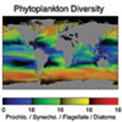The mechanisms that determine the relationship between diversity and productivity in marine phytoplankton remain unclear. Here, Vallina et al. show that selective predation and transient competitive exclusion determine phytoplankton community composition.

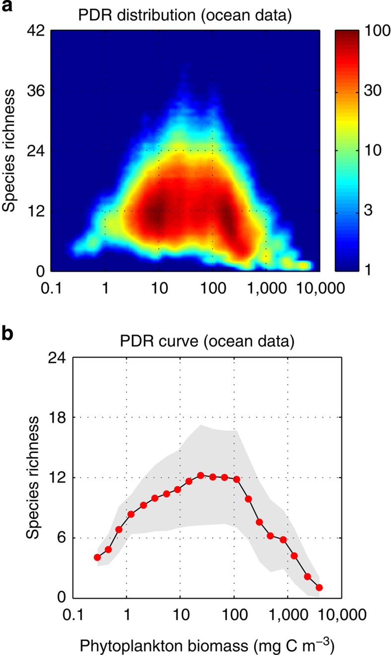
The relationship between diversity and productivity has been under strong debate during the last few decades1. Strictly speaking, productivity gives the biomass-specific growth rate (that is, inverse of duplication time) of a population or trophic level, but most empirical studies use biomass production or standing biomass as surrogate measures2. Large meta-analyses of terrestrial and aquatic ecosystems suggest that the shape of the productivity–diversity relationship (PDR) is generally either positive or unimodal3,4,5,6,7. For marine phytoplankton, there are less data available but a few large-scale studies also suggest an unimodal PDR response with maximum diversity peaking at intermediate levels of productivity and minimum diversity during massive blooms that escape grazing predation (see Fig. 1)8,9. Although these results are once again under debate owing to methodological concerns10,11, the exact mechanism(s) leading to positive or unimodal PDR remain unclear12. One way forward is to better understand the mechanistic processes that explain the patterns10. The shape of the PDR will ultimately reflect the mechanism(s) of species coexistence, and unimodal PDRs suggest dynamic, non-equilibrium processes13.

Figure 1. Global PDR from ocean field data sets.

(a) Global PDR distribution using Gaussian random sampling of the raw data69. (b) Global PDR curve using equally spaced log10 bins of biomass. Units: phytoplankton biomass (mg C m⁻³) and diversity (# species) (contributing >1% to total biomass).

Theoretical studies have suggested many productivity-drives-diversity hypotheses14 including the intermediate disturbance hypothesis15,16; the species-energy theory (SET)17; the resource-supply ratios hypothesis (RSR)18,19; the combined multi-variate hypothesis20; or the keystone-predation hypothesis (KPH)21. They all address different and complementary aspects of the PDR but their applicability to the marine environment is probably limited (see Methods). There is also the alternative view that diversity drives productivity, which is central to the field of biodiversity and ecosystem functioning22,23. Both points of view are currently seen as complementary rather than mutually exclusive20. Either way, the mechanisms of species coexistence need to be established to understand the consequences of diversity for ecosystem functioning22.

A mechanism for stable coexistence is the presence of a dynamic trade-off between competition ability for growth and vulnerability to mortality among the competing species24, which can result from selective predation25,26, selective viral lysis27,28 or both29. Here we focus on selective predation. Strategies leading to a higher resource competition ability in a given environment are assumed to concurrently increase the vulnerability to attacks by selective consumers according to a killing-the-winner (KTW) functional response30, which is a form of negative frequency-dependent selection31. Selective predation can arise from fully specialized predators (for example, prey specificity)32,33 or from behavioural changes of otherwise generalist predators (for example, prey switching)34,35. Switching towards alternative prey has been documented in natural ecosystems35,36,37,38 and is a predatory strategy that stabilizes foodwebs26,39,40. Preferentially attacking the dominant species provides a self-regulating negative feedback: the winners are downregulated by the predators while the losers are upregulated by granting them a predatory refuge30. Thus selective grazing allows predator-mediated coexistence24.

Selective feeding is a well-developed theoretical body that explains the rules of community assembly at equilibrium24,32,33,41. However, its role on the PDRs has never been evaluated for non-stationary systems such as the marine environment. Relatively little work has been done to explain global patterns of plankton diversity8,9,11. Scale is an essential component of ecological theory, because the response of dependent variables can change across multiple spatial and temporal scales13,42. Therefore, in this work we address the following two questions: (1) what are the mechanisms leading to an unimodal shape of the global PDR? (2) does the shape of the PDR change with the temporal scale of observation? The goal is to link mechanisms with theoretical predictions of observable patterns. We use a global marine ecosystem model that includes selective grazing by generic zooplankton, and we obtain a global ocean PDR at two temporal scales: annually (that is, 365 days) and weekly (that is, 5 days) averaged data.

The results are linked to the theory of phytoplankton community assembly for both equilibrium and non-equilibrium dynamics. We show that the unimodal PDR arises from a combination of top-down (selective grazing) and bottom-up (competition for nutrients) controls. The positive side is due to predator-mediated coexistence and is observed at both annual and weekly timescales, while the negative side is due to competitive exclusion by blooms of opportunist species and is only observed at the weekly scale because it captures transient non-equilibrium dynamics. The community composition of the positive and negative sides is mostly dominated by small and large phytoplankton, respectively.

Results

Productivity and diversity

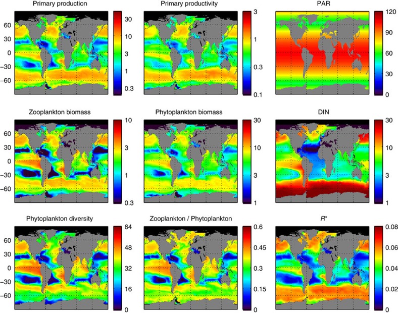
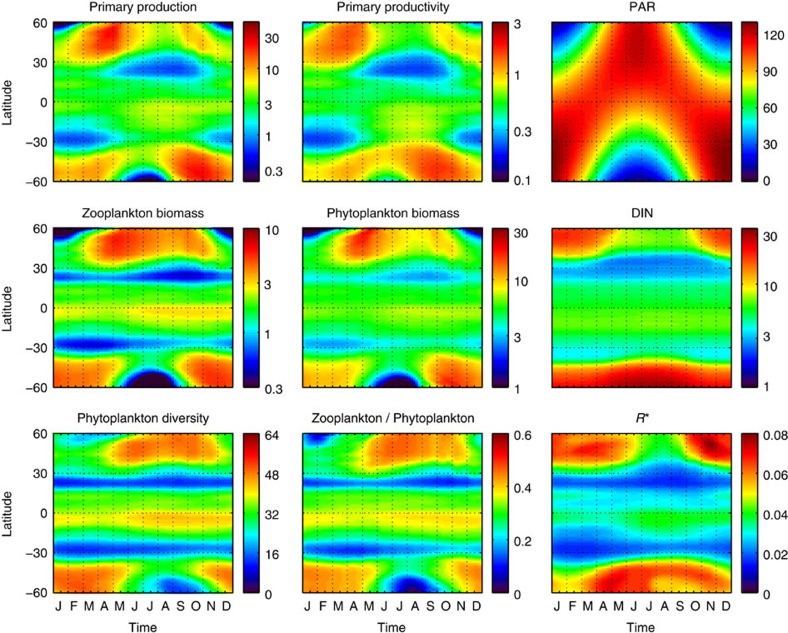
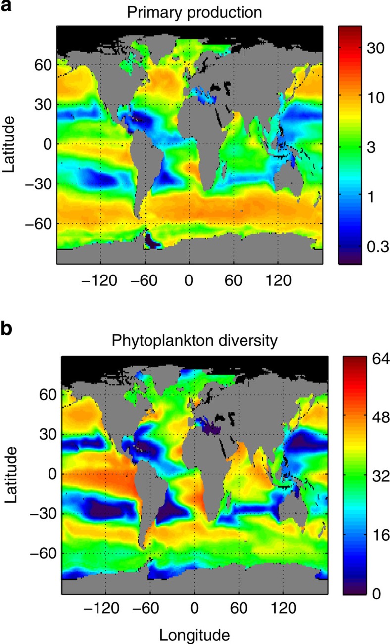
The model includes 64 phytoplankton species belonging to two size-classes and four major functional groups (that is, 16 species per group) that compete for several elemental nutrients and are grazed by two zooplankton size-classes, which feed preferentially on small and large phytoplankton, respectively, with KTW-selective feeding (see the Methods section). Primary production (mmol C m⁻³ d⁻¹) is strongly correlated (Spearman’s ρ>0.90) to primary productivity (d⁻¹), so we will use it as surrogate (see Figs 2 and 3). The simulated primary production captures well-known patterns of higher primary production over temperate zones and upwelling regions, as well as lower primary production over the oligotrophic subtropical gyres of the Pacific and Atlantic Oceans43 (see Fig. 4a). The model also captures the typical seasonal dynamics of primary production, which depends on latitude and is characterized by low seasonality at the equator and high seasonality over temperate zones, where there is a primary spring bloom and a secondary autumn bloom (see Fig. 5a). Primary production and phytoplankton diversity show a large degree of spatial correlation, with diversity tending to be higher where productivity is high and lower when productivity is low (see Fig. 4). However, they show a lesser degree of temporal correlation, with diversity tending to peak later than productivity, especially at higher latitudes (see Fig. 5).

Figure 2. Global ocean maps of annually averaged model outputs.

Primary production (mmol C m⁻³ d⁻¹); primary productivity (d⁻¹); photosynthetic active radiation (W m⁻²); zooplankton concentration (mmol C m⁻³); phytoplankton concentration (mmol C m⁻³); dissolved inorganic nitrogen (mmol N m⁻³); phytoplankton diversity (# species) (contributing >1% to total biomass); zooplankton/phytoplankton concentration ratio (n.d., no dimensions); subsistence nutrient concentration at equilibrium (R*) (mmol N m⁻³).

Figure 3. Hovmoller diagrams of model outputs (that is, time evolution of zonal averages).

Primary production (mmol C m⁻³ d⁻¹); primary productivity (d⁻¹); photosynthetic active radiation (W m⁻²); zooplankton concentration (mmol C m⁻³); phytoplankton concentration (mmol C m⁻³); dissolved inorganic nitrogen (mmol N m⁻³); phytoplankton diversity (# species) (contributing >1% to total biomass); zooplankton/phytoplankton concentration ratio no dimensions (n.d.); subsistence nutrient concentration at equilibrium (R*) (mmol N m⁻³).

Figure 4. Global ocean maps of annually averaged model outputs.

(a) Primary production (mmol C m⁻³ d⁻¹); (b) phytoplankton diversity (# species) (contributing >1% to total biomass).

Figure 5. Hovmoller diagrams of model outputs (that is, time evolution of zonal averages).

(a) Primary production (mmol C m⁻³ d⁻¹); (b) phytoplankton diversity (# species) (contributing >1% to total biomass).

Global PDR

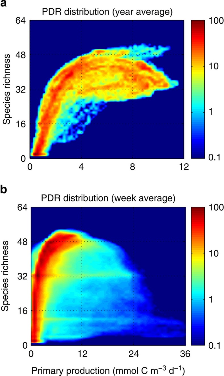
We consider the global PDR distributions obtained by plotting the global maps of phytoplankton diversity as a function of primary production using two different temporal averaging: annually averaged data (Fig. 6a) and weekly averaged data (Fig. 6b). The PDR distribution obtained with the annually averaged data (that is, using the maps of Fig. 4) confirms that diversity and productivity are strongly spatially correlated at the global scale (Fig. 6a). Diversity first increases linearly with primary production at low production regimes and then it saturates at higher primary production. Phytoplankton production is essentially reflecting the resource supply into the ecosystem. Annually averaged data are closer to a steady state, and at equilibrium primary production is directly linked to the net supply of the limiting resource24,44. Therefore phytoplankton diversity increases with the resource supply until it saturates.

Figure 6. Global PDR distribution of model outputs.

(a) Using annually averaged data; (b) using weekly averaged data. Units: primary production (mmol C m⁻³ d⁻¹); phytoplankton diversity (# species) (contributing >1% total biomass). Colour legend: the colourmap scale gives the relative (%) data density.

These results are driven by selective predation from the zooplankton community32,45. Competition among phytoplankton species at equilibrium obeys the resource competition theory18,46, and in the absence of selective feeding from herbivores the species with the lowest subsistence nutrient concentration (R*) outcompetes all others24. When zooplankton feeding is based on selective predation, however, dominant species will suffer a proportionally larger predation pressure than weaker competitors, which leads to a competition–vulnerability trade-off between the competing species33,30. Selective predation thus leads to a positive complementarity effect among the prey, which allows their predator-mediated coexistence24. Under these conditions, increasing the nutrient supply allows inferior competitors to persist in the system24,32,41,45.

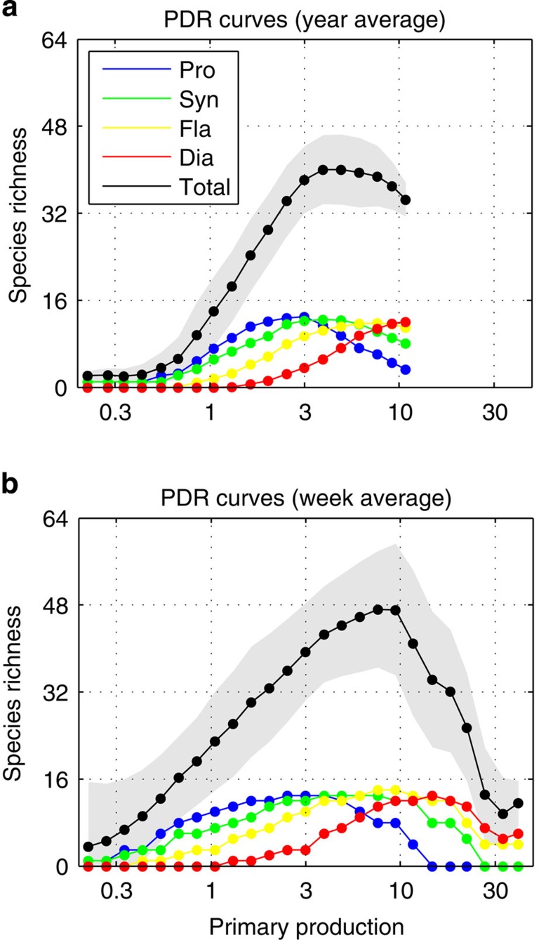
The PDR distribution obtained with weekly averaged data also shows a similar positive relationship between diversity and productivity over the range of primary production values spanning the annual averages, and most of the data points lie on this side of the distribution (Fig. 6b). However, for higher values of primary production the phytoplankton diversity can drop to very low values. The PDR curve for the annual data is clearly positive but heading to unimodal (see Fig. 7a) while the PDR curve for the weekly data is fully unimodal (see Fig. 7b). This reflects seasonally transient blooms of fast-growing species (for example, diatoms) that occur at the beginning of the growing season at high latitudes before their populations are downregulated by selective predation (see Fig. 5). There is a short temporal lag (<2 weeks) between the beginning of the growing season for phytoplankton and their predators (see Fig. 3). During that temporal window the fast-growing opportunists can bloom and outcompete all other species via exploitative resource competition9. This is particularly so for regions of strong seasonality47 with long darker winters during which plankton population densities are low while nutrient concentrations build up until solar radiation becomes less limiting. However, these are short-lived transient events; once the predator community catches up with the blooming species they will be downregulated and predator-mediated coexistence will re-appear. Thus these transient events only represent a relatively minor fraction of the total data points of the PDR distribution.

Figure 7. Global PDR curve of model outputs using equally spaced log10 bins of primary production.

(a) Using annually averaged data; (b) using weekly averaged data. Units: primary production (mmol C m⁻³ d⁻¹); phytoplankton diversity (# species) (contributing >1% total biomass). Colour legend: Prochlorococcus (blue line), Synechococcus (green line), flagellates (yellow line) and diatoms (red line).

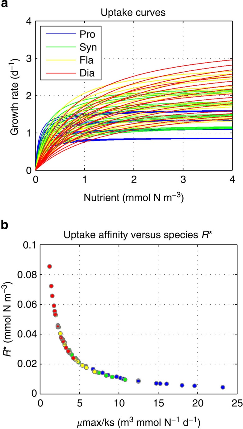
The same PDR patterns as for total diversity are observed for each phytoplankton group individually, but there is a succession in the diversity levels for each group as a function of productivity regardless of the temporal scale of observation (see colour lines in Fig. 7). Slow-growing nutrient specialists have their diversity peak at low production while fast-growing nutrient opportunists have their diversity peak at high production (see average R* of the phytoplankton community in Figs 2 and 3). This pattern reflects the growth–affinity trade-off that exists among the phytoplankton functional groups, which provides each group with a particular nutrient niche from low to high concentrations (see Fig. 8a and Methods). Competitive exclusion of species thus happens more strongly among than within phytoplankton functional groups, with each group tending to dominate over different oceanic regions according to their competitive abilities for nutrient uptake30.

Figure 8. Phytoplankton species traits that define their nutrient niches and competitive abilities.

(a) Species nutrient uptake curves as a function of dissolved inorganic nitrogen (mmol N m⁻³); (b) species subsistence nutrient concentration at equilibrium (R*) versus their nutrient uptake affinity (μmax/ks).

Community structure

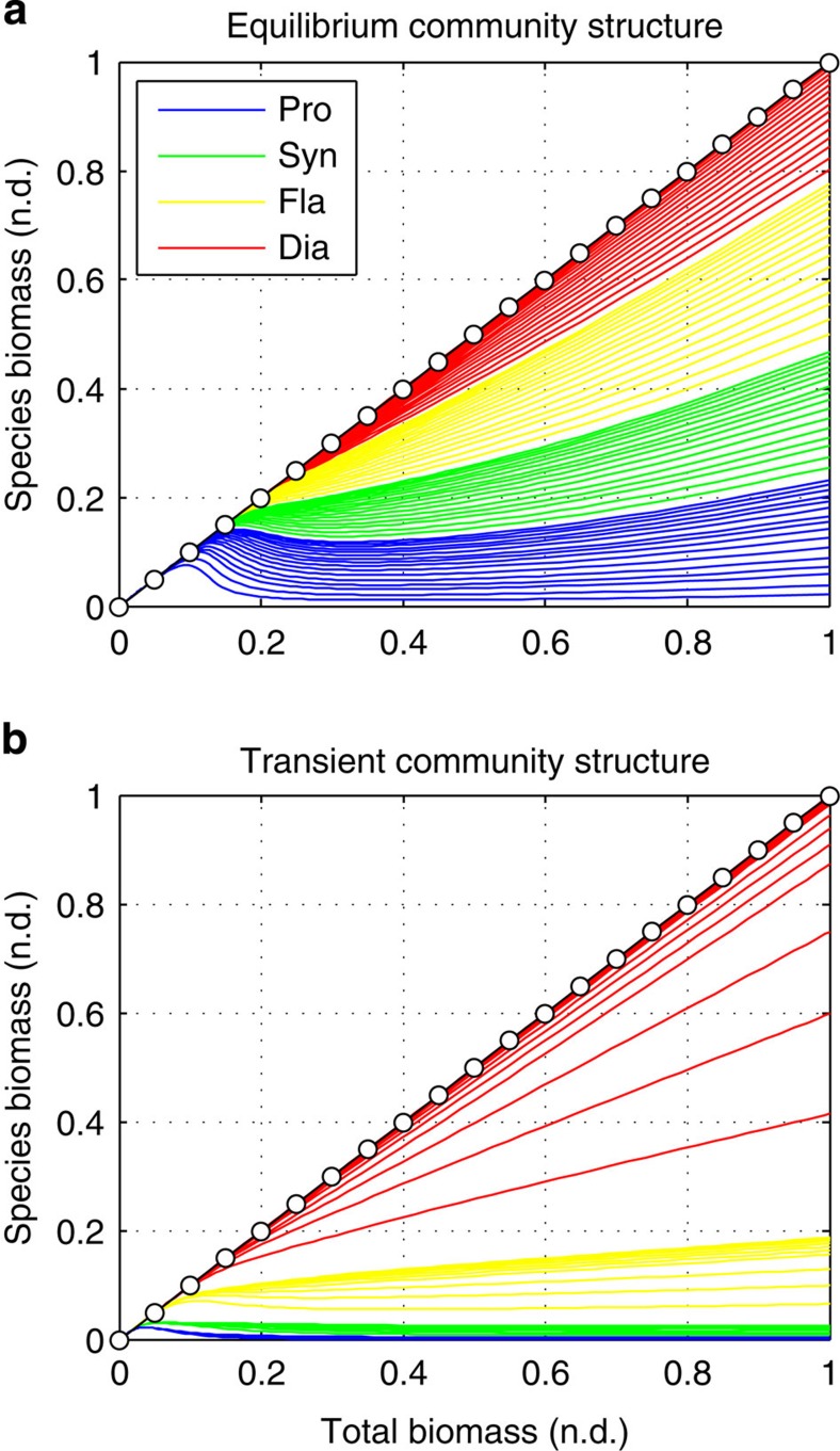
Using an idealized ecosystem without ocean dynamics and only one single essential nutrient (phosphorous), we evaluated phytoplankton community composition along an environmental gradient of increasing nutrient supply for both asymptotic steady-state equilibrium (see Fig. 9a) and short transient-state blooming conditions (see Fig. 9b). We performed 100 independent simulations and the gradient in nutrient supply was obtained by increasing the amount of total phosphorous in the system. Since each ecosystem is mass conservative, higher total phosphorous leads to higher nutrient supply and total phytoplankton biomass. This reproduces conditions that go from very oligotrophic to very eutrophic systems. The only external forcing is the solar radiation. For the steady-state case, we assume full solar radiation levels for the whole duration of the simulations. For the transient-state case, we performed periodic perturbations of the solar radiation levels with 2-month-long full-dark/light pulses. Only the first 2 weeks (that is, 10 days) of the full-light pulses were used to evaluate the community structure under blooming conditions exclusively.

Figure 9. Community structure along an environmental gradient of increasing nutrient supply.

(a) Steady-state equilibrium; (b) transient non-equilibrium. Species biomasses are cumulative on the y axis. Units: phytoplankton (normalized) biomass no dimensions (n.d.). Colour legend: Prochlorococcus (blue line), Synechococcus (green line), flagellates (yellow line) and diatoms (red line).

The steady-state community structure at lowest nutrient supply has only one slow-growing nutrient specialist with the lowest R* of all the phytoplankton species (see Figs 8b and 9a). Total phosphorous, nutrient supply and primary production are so low that predators cannot grow. In the absence of predators, therefore, this species, which is the strongest competitor at equilibrium (that is, it has the lowest R*), outcompetes all others32,48. Once the nutrient supply reaches a minimum critical value, the predator community can be sustained and starts to downregulate the abundance of the strongest phytoplankton competitor. At the same time the KTW-selective predation becomes significant and thus less competitive species can grow and persist in the system along the gradient of nutrient supply. The fast-growing opportunists have the highest R* and therefore they are the last species to successfully coexist in the system. For the highest nutrient supply most of the species are able to coexist and the biomasses of each phytoplankton group are roughly the same. Similar results have been shown for planktonic foodweb models based on size-specific predator–prey interactions using both an idealized ecosystem32 and a more realistic global ocean model48. Thus, selective feeding by an otherwise generalist community of predators has qualitatively the same effect on the prey community structure as many specialized communities of predators30.

The transient-state community structure, however, shows a different community structure that could not have been predicted by the steady-state theory outlined above (see Fig. 9b). With the exception of very low nutrient supply in which only a few slow-growing nutrient specialists can survive, for most of the nutrient supply range the phytoplankton community becomes dominated by fast-growing opportunists that totally outcompete the slow-growing specialists, despite having much larger R* than them. This result has previously been found in a global configured model47. Particularly for the highest nutrient supply, virtually all the total phytoplankton biomass belongs to fast-growing opportunists and the degree of total phytoplankton diversity is quite low when compared with the steady-state community structure. During the first full-light days after a long 2-month dark pulse, the conditions are optimal for the fast-growing species regardless of their equilibrium R*, because when nutrients are high they grow the fastest (see Fig. 8a). This leads to a transient uncontrolled bloom that cannot be sustained for long before nutrients run out and/or predatory mortality becomes significant. Therefore, the steady-state community structure explains the positive side of the PDR obtained with the global ocean simulation while the transient-state community structure explains its negative side.

Discussion

The relationship between diversity and productivity has been an object of extensive research for both terrestrial and aquatic ecosystems, but the debate is yet far from closed2,10. The global diversity patterns observed for marine phytoplankton show an unimodal relationship with productivity using phytoplankton biomass as surrogate9. However, this observation has been questioned owing to methodological concerns11. Rare species with low population abundances can go undetected in small (conventional) sampling volumes biasing the estimates of diversity towards common species. Although rare species can contribute significantly to total community diversity, their contribution to total primary production is relatively low. This has led to propose the idea that total diversity and productivity are not linked mechanistically11. Alternatively, one can estimate diversity including only common species (for example, contributing >1% of total community biomass), which are more likely to be regulated by resource supply and predatory pressures. The PDR obtained using this threshold is clearly unimodal for both field data (see Fig. 1) and global ocean simulations (Figs 6 and 7).

The debate about the shape of the PDR is very closely related to the debate about the mechanisms of species coexistence14 since the maintenance of species diversity is a necessary condition for a PDR. The presence of functional trade-offs among species has been suggested as an important element of the community composition along environmental gradients49. Growth–affinity trade-offs permit non-equilibrium coexistence in spatially heterogeneous and temporally fluctuating environments, because variability of the nutrient supply allows niche differentiation between the competing species24,47. Stable-equilibrium coexistence can further be achieved when predators impose a competition–vulnerability trade-off upon the competing species, which leads to predator-mediated complementarity between winners and losers33. Selective grazing has long been recognized to follow complex behavioural patterns50. Switching can result from behavioural changes that increase the attack rate on selected prey through a learning and feeding strategy34,35. Several factors such as prey size, morphology, abundance and nutritional quality can determine the preference for particular prey types50. Prey relative abundance is commonly used as a simple measure of species ecological success and thus of their vulnerability to consumer-induced mortality through density-dependent predation51. According to the optimal foraging theory, a low probability of capturing a given prey type relative to others should make it less appetizing because searching time may be better spent looking for alternative prey that provide higher return per foraging energetic investment52.

These two trade-offs are the mechanisms that maintain species diversity in our ecosystem model. The growth–affinity trade-off (bottom-up control) allows non-equilibrium coexistence of the four phytoplankton functional groups ranging from nutrient specialists to nutrient opportunists. The competition–vulnerability trade-off (top-down control) allows stable predator-mediated coexistence of phytoplankton species within and across functional groups. Under these conditions of species coexistence, our model predicts that the global PDR for marine phytoplankton depends on the temporal scale of observation, being positive at annual timescales and unimodal at weekly timescales. Nevertheless, the positive side of the curve dominates in terms of data density regardless of the temporal scale. Therefore the unimodal PDR curve for the total phytoplankton community arises from a combination of both top-down (that is, selective predation) and bottom-up (that is, competition for nutrients) controls. The PDR’s positive side is due to stable predator-mediated coexistence, and the PDR’s negative side is due to transient competitive exclusion by seasonal blooms of a few opportunists.

The model shows that at low nutrient supply, both productivity and diversity are low because only a few slow-growing specialists with high affinity for nutrients can grow under strong nutrient limitation for long periods of time; at intermediate nutrient supply, diversity increases because several slow-growing specialists and fast-growing opportunists can grow and coexist controlled by selective predation under more favourable conditions for long periods of time; and at high nutrient supply, productivity increases while diversity decreases because a few fast-growing opportunists can grow uncontrolled by predators (that is, bloom) during short periods of time during which they outcompete all other species. These results agree with the classical model proposed for unimodal PDR9,53. In this view, competition for nutrients drives both the lower and higher ends of the curve13. However, we also identify selective predation as the key mechanism that explains the positive side of the PDR at intermediate nutrient supply levels. Experimental manipulation of marine foodwebs on rocky shores has shown that the positive effect of nutrient supply on species diversity only happens in the presence of predators, because these mechanisms (that is, bottom-up versus top-down control) do not act in isolation, they need to be acting together in synergy54. Predation prevents competitively dominant prey from monopolizing resources, but only when grazing is preferentially directed towards the dominant species55.

Our simulations suggest that resource supply limits both phytoplankton productivity (directly) and diversity (indirectly, through predator-mediated complementarity). Thus, resource supply provides an upper limit to the amount of species that can coexist in a local community, and diversity will in turn determine how efficiently the resources are utilized for a given resource supply regime56. Nutrient supply influences primary production through covariation with both algal biomass and algal mass-specific productivity. When resource supply rates are constantly so low or temporarily so high that they encourage competitive exclusion, the phytoplankton community becomes dominated by a few superior competitors; when resource supply rates are sufficient to allow predator-mediated coexistence, the community becomes colonized by species that are able to use the resource in a complementary way. This means that the PDR obtained with selective predation contains both the complementarity and selection effects24,56, although they tend to operate at different productivity regimes and temporal scales. Therefore selective predation gives support to the view that the diversity of a local community will be determined by the potential productivity (that is, nutrient supply) while the actual productivity of the ecosystem will be determined by the diversity and species identity of the local community20. The role of selective predators then becomes a new key element of the phytoplankton community assembly.

Methods

KTW predation

We derived a KTW functional response by assuming that the predators’ attack rate upon a given prey species depends on its relative abundance. The attack rate upon each species is higher than the background (that is, basal) attack rate if they are relatively more abundant, and lower than the background if they are relatively less abundant. Thus, dominant species with higher relative abundance will suffer a proportionally larger predation pressure than weaker competitors with lower relative abundance. The formal mathematical derivation can be found in30. The final simplest expression that gives the ingestion rate upon a single prey species j is given in Fig. 10.

Figure 10. KTW functional response.

Gj is the grazing rate upon prey species j (mmol m⁻³ d⁻¹); Q^j_switching gives the fraction of prey species j in the predators' diet (n.d.); Q_feeding gives the overall feeding probability of predators (n.d.); V_max gives the maximum ingestion rate (mmol m⁻³ d⁻¹); g_max is the maximum specific rate for ingestion (d⁻¹); k_sat is the half-saturation constant for ingestion (mmol m⁻³); Z is the concentration of predators (mmol m⁻³); Pj is the concentration of prey species j (mmol m⁻³); ρj is a constant prey preference (n.d.); β is the Hill coefficient that measures how the feeding rate varies with total prey density no dimensions (n.d.); and α is the KTW coefficient that gives the potential for selective predation: when α=1.0 there is no switching (for example, passive filter feeding); when α>1.0 there is prey switching (that is, active selective predation).

Global ocean ecosystem model

We implemented the KTW functional response described above in a global marine ecosystem model47,57 to evaluate the influence of selective grazing on the shape of the global PDR for marine phytoplankton. The three-dimensional global ocean model is based on a coarse resolution (1° × 1° horizontally, 24 levels vertically) of the MIT general circulation model (MITgcm). The multi-species ecosystem model of two lower trophic levels (that is, phytoplankton and zooplankton) is coupled to the three-dimensional ocean physics such that organisms are passively transported by the fluid through advection and turbulent mixing (both vertical and horizontal). The coupled biophysical model was run for 8 years to reach (quasi) steady-state seasonal cycles. The model setup is the same as in ref. 30 and we direct the reader to the online supplemental material of that paper for additional discussion and information (for example, model parameter values).

The model was initialized with 64 phytoplankton species belonging to two size-classes and four major phytoplankton functional groups: 32 small phytoplankton (that is, 16 Prochlorococcus and 16 Synechococcus) and 32 large phytoplankton (that is, 16 flagellates and 16 diatoms). Functional grouping was based on nutrient requirement and uptake strategies. Regarding the nutrient requirement, all groups use phosphate, ammonium and iron. Diatoms are the only group requiring silica. Prochlorococcus analogues are here limited to ammonium as their sole source of nitrogen, although in nature some strains can also utilize nitrate. Synechococcus, flagellates and diatoms are assumed to take up ammonium preferentially over nitrate44. Regarding the uptake strategy, there is a continuous transition from strong competitive specialist to strong opportunist with the following order: Prochlorococcus, Synechococcus, flagellates and diatoms (see Fig. 8).

Phytoplankton diversity is defined as the number of species contributing >1% of the total biomass locally, which provides a measure of species richness that excludes rare species. The model also resolves two predator size-classes that feed preferentially (although not exclusively) on small and large phytoplankton, respectively: generic micro- and meso-zooplankton communities. Higher trophic levels are not explicitly modelled. Zooplankton losses owing to consumption by higher predators are implicitly modelled using a squared background mortality (that is, closure term). Phytoplankton growth is limited by four elemental nutrients (P, N, Fe and Si) and solar radiation. Background mortality, exudation, light harvesting and so on are common to all phytoplankton species.

Each phytoplankton species has a unique nutrient uptake curve (see Fig. 8a). Among groups, there is a growth–affinity trade-off that provides each phytoplankton functional group a particular nutrient niche ranging from slow-growing nutrient specialists with high affinity for uptake but low maximum growth (that is, Prochlorococcus and Synechococcus) to fast-growing nutrient opportunists with high maximum growth but low affinity for uptake (that is, flagellates and diatoms)47. Within groups, we generated 16 species by allowing a ±30% variability of the two traits that characterize the groups’ competition ability for nutrients: the maximum specific growth rate μmax (d⁻¹) and the half-saturation constant for nutrient uptake ks (mmol m⁻³). Within each group, the most competitive species will be the one having the highest maximum specific growth rate with the lowest half-saturation constant, which leads to the highest uptake affinity (that is, μmax/ks) and lowest R* (see Fig. 8b).

Model limitations and generality

Ecosystem models are by design simplifications of reality that seek to capture the main mechanisms that are thought to control species interactions both among them and with their local environment. Thus the model assumptions have a significant impact on their results. For example, our model ignores luxury uptake and storage capacity by phytoplankton cells, which can lead to competitive advantage under intermittent pulses of nutrient supply58. Droop quota models of phytoplankton growth can capture these dynamics, which can be relevant for community assembly particularly at small spatial and temporal scales (that is, submesoscale processes) while more classical Monod models do not capture them because they assume that uptake and growth are instantaneously coupled59,60.

However, given the usually coarse spatial resolution and low frequency of environmental forcing variability of global ocean simulations, Droop- and Monod-based models are expected to provide similar predictions. Furthermore, storage specialists can also be the fastest growing species; diatoms usually have the greatest luxury uptake and storage capacity of all major phytoplankton functional groups, which means that they will be the best competitors during high nutrient supply under both Monod and Droop kinetics. Therefore including luxury uptake and storage capacity would simply contribute to further strengthen the suggested role of transient blooms of opportunistic diatoms on the negative slope of the PDR at high productivity.

Our marine ecosystem model does not include an explicit representation of bacterial activity. The effect of the microbial loop is included through constant degradation rates of bacterial remineralization. That is, mortality and exudation losses are recycled to inorganic nutrients via constant rate degradation of several pools of organic matter (dissolved and particulate) for each essential element. This approach captures first-order dynamics of the microbial loop and provides a balance between model complexity and ecosystem realism. Modelling bacterial activity explicitly would increase the model’s realism at capturing the microbial foodweb dynamics, but it should not significantly change our results since bacterial abundances are generally more stable than phytoplankton abundances seasonally in open-ocean waters61.

Higher trophic levels are not explicitly modelled in our ecosystem model. Zooplankton losses owing to consumption by higher predators are implicitly modelled using a squared background mortality term. Quadratic mortality is one of the simplest closure terms; it assumes a predator whose biomass is proportional to that of the zooplankton. Since predator populations usually vary with those of their prey, this assumption is more realistic than the alternative approach of assuming a linear mortality. Under conditions where food availability is not limiting, the use of a squared mortality becomes equivalent as imposing a carrying capacity on the zooplankton community above which mortality loses by predation are higher than growth and then the population declines. Thus squared mortality has a tendency to stabilize foodwebs62.

Classical productivity–diversity theories

For non-equilibrium conditions, the most cited theory is the intermediate disturbance hypothesis15,16, because both diversity and productivity can be affected by environmental disturbances63. When species compete for space as the main resource, competitive exclusion can be prevented by periodic physical disturbance or mortality events caused by consumers as long as there is a trade-off between competitive ability and patch colonization rate54. However, competition for space is unlikely in phytoplankton species given the small size of the cells in relation to the water masses. Nevertheless, intermediate levels of environmental disturbance can lead to temporal and spatial heterogeneities that can certainly promote the local non-equilibrium coexistence of species that exhibit trade-offs in their competitive abilities14,24.

For equilibrium conditions, there are at least three major theories that rely on a different set of assumptions: they are the SET17; the RSR hypothesis18,19; and the KPH21. The SET predicts a positive PDR that saturates at high energy (that is, high resource) supply. This is explained using stochastic demography arguments: species population sizes increase as a function of resource supply, which decreases the probability of random extinctions of rare species20. However, the SET does not explicitly address what are the mechanisms of species coexistence at any level of resource supply and more precisely how can competitive exclusion64 be avoided as the population sizes increase. This makes the theory incomplete to explain the PDR curves of competitive plankton foodwebs.

The RSR predicts a unimodal PDR where diversity peaks at intermediate levels of a stoichiometrically balanced supply of non-substitutable resources. This theory explains local stable coexistence through species complementarity in their resource use20. Stable coexistence requires, however, a significant number of conditions: (1) each species has to be the best competitor for one of the resources; (2) each species has to consume proportionally more of the resource that limits its own growth more; (3) the supply rate of each resource has to be intermediate and balanced with respect to the other resources24. This means that there cannot be more coexisting species than the number of essential resources18. Phytoplankton cells are suspended in a generally well-mixed medium and compete for the same resources from a common and spatially homogeneous pool, which implies that all individuals are potentially interacting with each other65. Therefore, the RSR hypothesis can hardly explain the paradox of the plankton because there is a much larger number of coexisting species than of non-substitutable resources (for example, elemental nutrients) in the ocean66.

The KPH predicts a unimodal PDR through a mechanism that involves the modification of the degree of competition among primary producers by keystone predators due to a trade-off between the resource exploitation ability and the vulnerability to predators of the competing prey. Competing species interact via two mechanisms: they compete for a common pool of resources via exploitative competition and they interact via the apparent competition that occurs through the shared common predator67. At low productivity, vulnerable but good resource exploiters dominate because predators are absent or rare (that is, resistant species are excluded through direct resource competition); at high productivity, resistant but poor resource exploiters dominate because predators are very abundant (that is, resource exploiters are excluded through indirect apparent competition); at intermediate productivity, both types of strategies can coexist68. However, this model predicts a replacement series involving multiple pairs of species ranging from good resource exploiters to predator-resistant forms as productivity increases21. That is, for any given productivity the stable coexistence involves a maximum of two prey species. Therefore, the KPH can only explain the local coexistence of two species, which contrasts with the much larger degree of species coexistence explained by KTW-selective feeding. This is because the KPH assumes that the trade-off between resource exploitation ability and vulnerability to predators of the competing prey is fixed, while the KTW-selective feeding assumes that it is variable depending on prey dominance.

Ocean field data

The global PDR from ocean field data (see Fig. 1) was obtained using a compiled data set of marine microplankton species abundances collected on different oceanographic cruises between 1992 and 2002 at 788 stations with an extensive geographical coverage69. Phytoplankton abundance (cell cm⁻³) was converted to phytoplankton biomass (mg C m⁻³) using a cell carbon-density factor of 0.25 (pg C μm⁻³)70. Phytoplankton diversity was computed as richness of species contributing >1% of total phytoplankton biomass (that is, rare species were not included). We performed a Gaussian random sampling upon the raw data to increase by a factor of × 1,000 the number of data points and thus statistical significance by assuming that both phytoplankton biomass and diversity are normally distributed variables. All data points were thus drawn at random from a Gaussian distribution centred at the mean observed (that is, measured) value μ and with s.d. σ=0.2 μ.

Author contributions

All authors have contributed extensively to the work. S.M.V. conceived the research, performed the computational work and wrote the article. P.C. contributed to the research design and the interpretation of the results. J.M.M. and M.L. supervised the data analysis and the interpretation of the results. M.J.F. and S.D. supervised the research project and the computational work. All authors assisted in the writing process and revised the manuscript.

Additional information

How to cite this article: Vallina, S. M. et al. Global relationship between phytoplankton diversity and productivity in the ocean. Nat. Commun. 5:4299 doi: 10.1038/ncomms5299 (2014).

References

- Strong D. R. Evidence and inference: shapes of species richness-productivity curves. Ecology 91, 2534–2535 (2010). [DOI] [PubMed] [Google Scholar]
- Groner E. & Novoplansky A. Reconsidering diversity-productivity relationships: directness of productivity estimates matters. Ecology Lett. 6, 695–699 (2003). [Google Scholar]
- Dodson S. I., Arnott S. E. & Cottingham K. L. The relationship in lake communities between primary production and species richness. Ecology 81, 2662–2679 (2000). [Google Scholar]
- Mittelbach G. G. et al. What is the observed relationship between species richness and productivity? Ecology 82, 2381–2396 (2001). [Google Scholar]
- Chase J. M. & Leibold M. A. Spatial scale dictates the productivity biodiversity relationship. Nature 416, 427–430 (2002). [DOI] [PubMed] [Google Scholar]
- Gillman L. N. & Wright S. D. The influence of productivity on the species richness of plants: a critical assessment. Ecology 87, 1234–1243 (2006). [DOI] [PubMed] [Google Scholar]
- Smith V. H. Microbial diversity-productivity relationships in aquatic ecosystems. FEMS Microbiol. Ecol. 62, 181–186 (2007). [DOI] [PubMed] [Google Scholar]
- Li W. K. W. Macroecological patterns of phytoplankton in the northwestern north Atlantic ocean. Nature 419, 154–157 (2002). [DOI] [PubMed] [Google Scholar]
- Irigoien X., Huisman J. & Harris R. P. Global biodiversity patterns of marine phytoplankton and zooplankton. Nature 429, 863–867 (2004). [DOI] [PubMed] [Google Scholar]
- Adler P. B. et al. Productivity is a poor predictor of plant species richness. Science 333, 1753 (2011). [DOI] [PubMed] [Google Scholar]
- Cermeno P. et al. Species richness in marine phytoplankton communities is not correlated to ecosystem productivity. Mar. Ecol. Prog. Ser. 488, 1–9 (2013). [Google Scholar]
- Korhonen J. J., Wang J. & Soininen J. Productivity-diversity relationships in lake plankton communities. PLoS ONE 6, e22041 (2011). [DOI] [PMC free article] [PubMed] [Google Scholar]
- Graham J. H. & Duda J. J. The humpbacked species-richness curve: a contingent rule for community ecology. Int. J. Ecol. 2011, 1–15 (2011). [Google Scholar]
- Palmer M. W. Variation in species richness: towards a unification of hypotheses. Folia Geobot. Phytotax. 29, 511–530 (1994). [Google Scholar]
- Connell J. H. Diversity in tropical rain forests and coral reefs. Science 199, 1302–1310 (1978). [DOI] [PubMed] [Google Scholar]
- Huston M. A. A general hypothesis of species diversity. Am. Nat. 113, 81–101 (1979). [Google Scholar]
- Wright D. H. Species-energy theory: an extension of species-area theory. Oikos 41, 496–506 (1983). [Google Scholar]
- Tilman D. Resource Competition and Community Structure Princeton Univ. Press (1982). [PubMed] [Google Scholar]
- Tilman D. The resource ratio hypothesis of succession. Am. Nat. 125, 827–852 (1985). [Google Scholar]
- Cardinale B. J., Hillebrand H., Harpole W. S., Gross K. & Ptacnik R. Separating the influence of resource 'availability' from resource 'imbalance' on productivity-diversity relationships. Ecol. Lett. 12, 475–487 (2009). [DOI] [PubMed] [Google Scholar]
- Leibold M. A. A graphical model of keystone predators in food webs: trophic regulation of abundance, incidence, and diversity patterns in communities. Am. Nat. 147, 784–812 (1996). [Google Scholar]
- Loreau M., Naeem S. & Inchausti P. Biodiversity and Ecosystem Functioning: Synthesis and Perspectives Oxford Univ. Press (2002). [Google Scholar]
- Duffy J. E. Why biodiversity is important to the functioning of realworld ecosystems. Front. Ecol. Environ. 7, 437–444 (2009). [Google Scholar]
- Loreau M. From Populations to Ecosystems: Theoretical Foundations for a New Ecological Synthesis Princeton Univ. Press (2010). [Google Scholar]
- Oaten A. & Murdoch W. W. Switching, functional response, and stability in predator-prey systems. Am. Nat. 109, 299–318 (1975). [Google Scholar]
- Murdoch W. W. & Oaten A. Predation and population stability. Adv. Ecol. Res. 9, 1–131 (1975). [Google Scholar]
- Thingstad T. F. Elements of a theory for the mechanisms controlling abundance, diversity, and biogeochemical role of lytic bacterial viruses in aquatic systems. Limnol. Oceanogr. 45, 1320–1328 (2000). [Google Scholar]
- Jover L. F., Cortez M. H. & Weitz J. S. Mechanisms of multi-strain coexistence in host–phage systems with nested infection networks. J. Theor. Biol. 332, 65–77 (2013). [DOI] [PubMed] [Google Scholar]
- Winter C., Bouvier T., Weinbauer M. G. & Thingstad T. F. Trade-offs between competition and defense specialists among unicellular planktonic organisms: the ‘killing the winner’ hypothesis revisited. Microbiol. Mol. Biol. Rev. 74, 42–57 (2010). [DOI] [PMC free article] [PubMed] [Google Scholar]
- Vallina S. M., Word B. A., Dutkiewicz S. & Follows M. J. Maximal feeding with active prey-switching: A kill-the-winner functional response and its effect on global diversity and biogeography. Prog. Oceanogr. 120, 93–109 (2014). [Google Scholar]
- Allen J. A. & Clarke B. C. Frequency dependent selection: homage to E. B. poulton. Biol. J. Linnean Soc. 23, 15–18 (1984). [Google Scholar]
- Armstrong R. A. Grazing limitation and nutrient limitation in marine ecosystems: steady-state solutions of an ecosystem model with multiple food chains. Limnol. Oceanogr. 39, 597–608 (1994). [Google Scholar]
- Thébault E. & Loreau M. Food-web constraints on biodiversity-ecosystem functioning relationships. Proc. Natl Acad. Sci. USA 100, 14949–14954 (2003). [DOI] [PMC free article] [PubMed] [Google Scholar]
- Murdoch W. W. The functional response of predators. J. Appl. Ecol. 14, 335–341 (1973). [Google Scholar]
- Kiorboe T., Saiz E. & Viitasalo M. Prey switching behaviour in the planktonic copepod Acartia tonsa. Mar. Ecol. Prog. Ser. 143, 65–75 (1996). [Google Scholar]
- Murdoch W. W. Switching in general predators: experiments on predator specificity and stability of prey populations. Ecol. Monogr. 39, 335–354 (1969). [Google Scholar]
- Gismervik I. & Andersen T. Prey switching by Acartia clausi: experimental evidence and implications of intraguild predation assessed by a model. Mar. Ecol. Prog. Ser. 157, 247–259 (1997). [Google Scholar]
- Kempf A., Floeter J. & Temming A. Predator-prey overlap induced Holling type III functional response in the North Sea fish assemblage. Mar. Ecol. Prog. Ser. 357, 295–308 (2008). [Google Scholar]
- Haydon D. Pivotal assumptions determining the relationship between stability and complexity: an analytical synthesis of the stability-complexity debate. Am. Nat. 144, 1 (1994). [Google Scholar]
- Armstrong R. A. Stable model structures for representing biogeochemical diversity and size spectra in plankton communities. J. Plankton Res. 21, 445–464 (1999). [Google Scholar]
- Grover J. P. Assembly rules for communities of nutrient-limited plants and specialist herbivores. Am. Nat. 143, 258–282 (1994). [Google Scholar]
- Levin S. A. The problem of pattern and scale in ecology. Ecology 73, 1943–1967 (1992). [Google Scholar]
- Behrenfeld M. J., Boss E., Siegel D. A. & Shea D. M. Carbon-based ocean productivity and phytoplankton physiology from space. Global Biogeochem. Cycles 19, GB1006 (2005). [Google Scholar]
- Vallina S. M. & Le Quéré C. Stability of complex food webs: resilience, resistance, and the average interaction strength. J. Theor. Biol. 272, 160–173 (2011). [DOI] [PubMed] [Google Scholar]
- Ward B. A., Dutkiewicz S., Jahn O. & Follows M. J. A size-structured food-web model for the global ocean. Limnol. Oceanogr. 57, 1877–1891 (2012). [Google Scholar]
- Tilman D. Resource competition between planktonic algae: an experimental and theoretical approach. Ecology 58, 338–348 (1977). [Google Scholar]
- Dutkiewicz S., Follows M. J. & Bragg J. G. Modeling the coupling of ocean ecology and biogeochemistry. Global Biogeochem. Cycles 23, GB4017 (2009). [Google Scholar]
- Ward B. A., Dutkiewicz S. & Follows M. J. Modeling spatial and temporal patterns in size-structured marine plankton communities: top-down and bottom-up controls. J. Plankton Res. 36, 31–47 (2014). [Google Scholar]
- Litchman E., Klausmeier C. A., Schofield O. M. & Falkowski P. G. The role of functional traits and trade-offs in structuring phytoplankton communities: scaling from cellular to ecosystem level. Ecol. Lett. 10, 1170–1181 (2007). [DOI] [PubMed] [Google Scholar]
- Wirtz K. W. Who is eating whom? morphology and feeding type determine the size relationship between planktonic predators and their ideal prey. Mar. Ecol. Prog. Ser. 445, 1–12 (2012). [Google Scholar]
- Gentleman W., Leising A., Frost B., Strom S. & Murray J. Functional responses for zooplankton feeding on multiple resources: a review of assumptions and biological dynamics. Deep-Sea Res. II 50, 2847–2875 (2003). [Google Scholar]
- Visser A. W. & Fiksen Ø. Optimal foraging in marine ecosystem models: selectivity, profitability and switching. Mar. Ecol. Prog. Ser. 473, 91–101 (2013). [Google Scholar]
- Rosenzweig M. L. & Abramsky Z. in:Species Diversity in Ecological Communities: Historical and Geographical Perspectives eds Ricklefs R. E., Schluter D. 52–65University of Chicago Press (1993). [Google Scholar]
- Worm B., Lotze H. K., Hillebrand H. & Sommer U. Consumer versus resource control of species diversity and ecosystem functioning. Nature 417, 848–851 (2002). [DOI] [PubMed] [Google Scholar]
- Lubchenco J. Plant species diversity in a marine intertidal community: importance of herbivore food preference and algal competitive abilities. Am. Nat. 112, 23–39 (1978). [Google Scholar]
- Cardinale B. J., Bennett D. M., Nelson C. E. & Gross K. Does productivity drive diversity or vice versa? a test of the multivariate productivity–diversity hypothesis in streams. Ecology 90, 1227–1241 (2009). [DOI] [PubMed] [Google Scholar]
- Follows M. J., Dutkiewicz S., Grant S. & Chisholm S. W. Emergent biogeography of microbial communities in a model ocean. Science 315, 1843–1846 (2007). [DOI] [PubMed] [Google Scholar]
- Cermeño P., Lee J. B., Schofield O. & Falkowski P. G. Competitive dynamics in two species of marine phytoplankton under non-equilibrium conditions. Mar. Ecol. Prog. Ser. 429, 1–28 (2011). [Google Scholar]
- Grover J. P. Resource competition in a variable environment: phytoplankton growing according to Monod’s model. Am. Nat. 136, 771–789 (1991). [Google Scholar]
- Grover J. P. Resource competition in a variable environment: phytoplankton growing according to the variable-internal-stores model. Am. Nat. 138, 811–835 (1991). [Google Scholar]
- Spitz Y. H., Moisan J. R. & Abbott M. R. Configuring an ecosystem model using data from the Bermuda Atlantic time series (bats). Deep-Sea Res. II 48, 1733–1768 (2001). [Google Scholar]
- Edwards A. M. & Yool A. The role of higher predation in plankton population models. J. Plankton Res. 22, 1085–1112 (2000). [Google Scholar]
- Grime J. P. Competitive exclusion in herbaceous vegetation. Nature 242, 344–347 (1973). [Google Scholar]
- Hardin G. The competitive exclusion principle. Science 131, 1292–1297 (1960). [DOI] [PubMed] [Google Scholar]
- Sommer U. in:Ecological Studies Vol. 161, eds Sommer U., Worm B. 79–108Springer (2002). [Google Scholar]
- Hutchinson G. E. The paradox of the plankton. Am. Nat. 95, 137–145 (1961). [Google Scholar]
- Holt R. D. Predation, apparent competition, and the structure of prey communities. Theor. Popul. Biol. 12, 197–229 (1977). [DOI] [PubMed] [Google Scholar]
- Leibold M. A. Biodiversity and nutrient enrichment in pond plankton communities. Evol. Ecol. Res. 1, 73–95 (1999). [Google Scholar]
- Sal S., Lopez-Urrutia A., Irigoien X., Harbour D. S. & Harris R. P. Marine microplankton diversity database. Ecology 94, 1658 (2013). [Google Scholar]
- Menden-Deuer S. & Lessard E. J. Carbon to volume relationships for dinoflagellates, diatoms, and other protist plankton. Limnol. Oceanogr. 45, 569–579 (2000). [Google Scholar]