Abstract
Cerenkov luminescence tomography (CLT) was developed to reconstruct a three-dimensional (3D) distribution of radioactive probes inside a living animal. Reconstruction methods are generally performed within a unique framework by searching for the optimum solution. However, the ill-posed aspect of the inverse problem usually results in the reconstruction being non-robust. In addition, the reconstructed result may not match reality since the difference between the highest and lowest uptakes of the resulting radiotracers may be considerably large, therefore the biological significance is lost. In this paper, based on the minimization of a conformance error, a probability method is proposed that consists of qualitative and quantitative modules. The proposed method first pinpoints the organ that contains the light source. Next, we developed a 0-1 linear optimization subject to a space constraint to model the CLT inverse problem, which was transformed into a forward problem by employing a region growing method to solve the optimization. After running through all of the elements used to grow the sources, a source sequence was obtained. Finally, the probability of each discrete node being the light source inside the organ was reconstructed. One numerical study and two in vivo experiments were conducted to verify the performance of the proposed algorithm, and comparisons were carried out using the hp-finite element method (hp-FEM). The results suggested that our proposed probability method was more robust and reasonable than hp-FEM.
OCIS codes: (100.3190) Inverse problems; (110.6960) Tomography; (170.3010) Image reconstruction techniques; (170.3660) Light propagation in tissues; (170.3880) Medical and biological imaging; (170.6280) Spectroscopy, fluorescence and luminescence
1. Introduction
Molecular imaging was designed to visualize the qualitative or quantitative measurements of biological processes at the molecular or cellular levels in vivo [1, 2]. The main advantage of molecular imaging lies in its ability to characterize diseased tissue without being invasive. Compared with other molecular imaging techniques, optical imaging has such advantages as nano–molar sensitivity, a high spatial resolution, a short imaging time, and low cost [3, 4]. Ever since Cerenkov radiation light was used by Cho et al. to perform direct optical imaging [5], Cerenkov imaging has been employed in molecular imaging. Unlike anatomical imaging, Cerenkov imaging is a type of functional imaging technique. When we deal with organs with the same density but different radiotracer uptakes, their anatomical imaging may be invalid; however, Cerenkov imaging can be used to distinguish them. Cerenkov imaging can be divided into two types: Cerenkov luminescence imaging (CLI) [6–16] and Cerenkov luminescence tomography (CLT) [17–26]. CLI is a type of 2D planar imaging, whereas CLT was developed to reconstruct the 3D distribution of radiotracers inside a living animal.
The CLT problem is an inverse one, which is the search for unknown sources through an analysis of the measured photon flux density on a boundary. A solution to the inverse problem can generally be divided into two types. One is a statistical method, e.g., a Monte Carlo [26, 27] or Bayesian [28, 29] method. The other is optimization using a least-squares criterion [18, 19, 30, 31], a regularization method [18–23], a level set method [32, 33], etc. As a new molecular modality, the methods used for CLT reconstruction are mainly focused on optimization.
Historically, the first extension of CLI to CLT was a homogeneous model based on the assumption that the optical properties inside a mouse are homogeneous and uniform [18]. The CLT model was solved iteratively using a preconditioned conjugate gradient method with Tikhonov regularization (TR) for bioluminescence tomography (BLT) [18, 30]. Because this assumption is not necessarily true, Hu et al. performed a heterogeneous CLT reconstruction [20], in which the adaptive hp-finite element method (hp-FEM) [34], originally designed for BLT, was employed for CLT reconstruction. In addition, finite element equations were also solved through TR. Both approaches employed a single band-pass filter. Spinelli et al. developed a multispectral method for CLT reconstruction [19], in which a regularized non-negative least square algorithm was designed for optimization [19, 31]. However, the detected multispectral data were weaker after the application of filters, which increased the difficulty in reconstructing the source. Hu et al. also proposed a hybrid spectral CLT method [21]. This method employed white light images for reconstruction without the use of a filter. The optical parameters were estimated by weighing four band-pass optical parameters, i.e., 515-575 nm, 575-650 nm, 695-770 nm, and 810-875nm at approximately 57.2%, 27.6%, 12.4%, and 2.8% respectively. After obtaining the optical parameters, the hp-FEM method [34] was also employed as a reconstruction method. Recently, Cerenkov excited tomography was designed for clinical interest [25, 26]. The Cerenkov excited tomography showed advances in the reconstruction of a deep target via Cerenkov photons.
A permissible region (PR) is usually used as the a priori information to improve the robustness of the finite element method (FEM) for diffuse optics reconstruction. In [22], the authors presented a single photon emission computed tomography (SPECT)-guided reconstruction method for CLT, in which a priori information of the permissible source region from the SPECT imaging results was incorporated to enhance the robustness of the reconstruction. Apart from the a priori information, when the TR method is employed to solve the optimization problem, an optimal can be another method to improve the robustness. It was reported that regularization was more suitable than regularization [35, 36].
These early reconstruction approaches were consistently committed to control errors to obtain a unique reconstruction. However, this was a difficult task. For this paper, we were committed to obtaining a non-unique description within the probability framework. A novel probability method for CLT based on conformance error minimization was designed in this work. It mainly contained two modules, i.e., qualitative and quantitative modules. A qualitative module gives an approximate estimation of the source by indicating a luminous organ. The quantitative module further describes the probability of the source location rather than seeking a unique solution of the photon density in that specified organ.
The five methodological contributions of this paper were as follows:
-
1)
A conformance error was provided for optimal assessment. This was beneficial to increase the robustness.
-
2)
A 0-1 linear optimization subject to a space constraint was used to model the CLT inverse problem.
-
3)
The inverse problem was transformed into a forward problem by employing a region growing method to solve the optimization.
-
4)
A probability source (PS), which offers a probability distribution of the nodes in the PR being a light source, was defined. The statistical description increased the reasonableness of the reconstruction.
-
5)
Comparison experiments demonstrated the advantages of the proposed method including its robustness, accuracy, and reasonableness.
The remainder of this paper is organized as follows. The related basis and hp-FEM are introduced in Section 2. In Section 3, the proposed method used for CLT reconstruction to improve the robustness and increase the reasonableness is presented in detail. The numerical and in vivo comparative experiments are described in Sections 4 and 5 respectively. Finally, a discussion and some concluding remarks are presented in Section 6.
2. hp-FEM
Conventionally, a photon transport in tissue can be modeled using a diffusion equation (DE) [34, 37–40]. The steady-state DE is modeled as , where is the photon flux density at point ; , and are the absorption and scattering coefficients respectively, is the anisotropy parameter, which can be obtained from optical sensing techniques [41–43]; denotes the internal source density; and is the region of interest (ROI).
The inverse problem has no unique solution. Theoretical studies on the non-uniqueness of the solution to the inverse model were reported in [44–46]. The non-uniqueness of the solution is due to the nature that the photon flux density is only partially known on the boundary . Therefore, the inverse problem is generally an ill-posed one.
Together with the Robin boundary condition, FEM was used to calculate the solution to DE [37–40]. In these studies, after a separation of the variables, the system equation of the DE was presented as follows [37–40]:
| (1) |
where is the nodal photon density measured on the boundary , is the permissible source vector, and is the coefficient matrix. The main outline of hp-FEM [34] is given in Algorithm 1.
Table 1. Optical parameters of the heterogeneous phantom.
| Material | Adipose | Lungs | Heart | Bone | Liver |
|---|---|---|---|---|---|
| 0.010 | 0.350 | 0.200 | 0.002 | 0.035 | |
| 4.000 | 23.000 | 16.000 | 20.000 | 6.000 | |
| 0.900 | 0.940 | 0.850 | 0.900 | 0.900 |
| Algorithm 1. The outline of hp-FEM algorithm, where p-refinement and h-refinement are subdivisions of a tetrahedron. | ||||
|---|---|---|---|---|
| Input: , , , , , | ||||
| do | ||||
| Form and solve the objective function: | ||||
| do | ||||
| Optimize | ||||
| Calculate the gradient norm | ||||
| Calculate the step distance | ||||
| while and | ||||
| Calculate | ||||
| p-refinement or h-refinement for selected elements | ||||
| Update the permissible region | ||||
| k = k + 1 | ||||
| while and | ||||
| Output: the reconstructed source | ||||
3. Proposed method
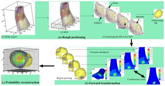
To improve the robustness of the reconstruction, we proposed a novel probability method based on conformance error minimization (shown in Fig. 1), which contained three modules: (1) rough positioning (Fig. 1(a)), (2) forward transformation (Fig. 1(b)), and (3) probability reconstruction (Fig. 1(c)). Among these three modules, module (1) is qualitative, whereas modules (2) and (3) are quantitative. The new method first pinpoints an organ that contains a light source. The well-known inverse problem is then transformed into a forward problem (e.g., Fig. 1(b5) results from Fig. 1(b1) using a forward calculation) using the region growing method (e.g., Fig. 1(b1)). The growth is controlled using the error between the measured surface photon density (MSPD) (e.g., Fig. 1(b9)) and the calculated surface photon density (CSPD) (e.g., Fig. 1(b5)). After running through all of the elements of the pinpointed organ, a source sequence is obtained (e.g., Fig. 1(b1)-1(b4)). Finally, the probability of each element node being the light source inside the organ is reconstructed and dyed with a pseudo-color after interpolation (Fig. 1(c)).
Fig. 1.
Outline of the probability method. (a) a rough positioning procedure. (a1) a mouse region bounded in . (a2) the region of interest (ROI) cropped from the mouse region and bounded in . (a3) the procedure for searching for the permissible region (PR). (a4) the resulting PR located in one of the organs inside the ROI. (b) a transformation of the inverse problem into the forward problem using the region growing method. Images (b1)-(b4) show examples of four grown sources after region growth. Images (b5)-(b8) show the normalized calculated surface photon density (CSPD) calculated by each corresponding grown source. (b9) shows the original measured surface photon density (MSPD) after normalization. (c) probability reconstruction of each element node being the light source inside the organ. The probability is dyed with a pseudo-color after interpolation.
3.1 Rough positioning
Rough positioning is a procedure for finding the correct organ containing a light source. The aim of rough positioning is to reduce the computation cost and increase the reconstruction robustness.
In this study, node number of the PR was chosen without exceeding node number on the boundary. Otherwise, Eq. (1) will end up with infinitely many solutions, and a minimal norm least square solution (Moore-Penrose generalized solution) is chosen as the approximation of the solution [47–50]. Although, the TR method is usually implemented to solve the underdetermined system in diffuse optics, this theoretically poses significant risk. The regularization is a numerical method used to approximate the Moore-Penrose generalized solution when Eq. (1) is an ill-posed problem [47, 48]. If the generalized solution is not the real solution among the infinitely many solutions, the numerical method is meaningless. On the contrary, the overdetermined system may result in a more robust result.
Suppose that a mouse body is region (Fig. 1(a1)), an ROI, denoted as , is then cropped from , as shown in Fig. 1(a2). The cropped part should contain the nonzero region of the MSPD. In our method, the PR is searched for in .
Let , where is an organ confined in . Assume that is the PR, is the permissible source vector, and is the corresponding coefficient matrix. To avoid infinitely many solutions, the cropped should satisfy , where and represent the number of nodes ofand respectively. From Eq. (1), source is reconstructed by
| (2) |
where is the MSPD on the boundary of .
After running through all of the , the PR can be defined when the conformance error reaches its minimum, the mathematic expression of which is as follows:
| (3) |
where the component of satisfies if , otherwise , is the jth component of , is the solution of Eq. (2) solved using the TR method, and , . After running through, the PR is determined using a minimum conformance error of Eq. (3). From this point, light source reconstruction is only carried out inside , which reduces the computational cost and increases the robustness significantly.
3.2 Forward transformation
In this step, the inverse problem is transformed into a forward problem using a region growing method. By assuming a certain element inside the PR to be the seed element, the growth is initiated to find the corresponding light source (e.g., Fig. 1(b1)). This procedure is repeated for all elements inside the PR, and finally the light source sequence is obtained (e.g., Fig. 1(b1)-1(b4)). The growth is controlled by the conformance error between the MSPD (Fig. 1(b9)) and the CSPD (e.g., Fig. 1(b5)-1(b8)).
For an easier presentation, we denote the PR as and the tied coefficient matrix as . Let be discretized into non-overlapping elements , where , is an element (tetrahedron), is the attached element vertices; and is the discrete vector of the permissible source. Because the absorption of drugs by different elements in the same organ is homogeneous if there is no excitation source [18], we suppose that the elements in the same organ have the same uptake of the tracer. A new quantitative model for reconstructing the source location and photon density is proposed as
| (4) |
subject to
-
1)
-
2)
Let be a set of all discrete source nodes. If is a source node, i.e., , then and one , such that .
The above optimization is a 0-1 linear programming problem. Because the aim of Eq. (4) is to search for a linear combination of columns in and obtain a maximum conformance between CSPD and MSPD , Eq. (4) together with constraint 1) is equivalent to finding a linear least square solution of equation , subject to , where is the value of the assumed uniform photon density resulting from the same radiotracer uptake inside the unit volume of .
Let be the singular value decomposition of, and thus, . In practice, is a full column rank; however, there are some small nonzero singular values. Let and be the maximal and minimal nonzero singular values, and the generalized condition number [51–53] is therefore very large under the norm, and is ill-posed. Therefore, the equivalent optimal model (4) might also be an ill-posed problem.
The regularization method, which frames the variable in a Hilbert space, is usually proposed to solve an ill-posed problem. However, unlike the continual model (2), the solution of the optimal model (4) is constrained as a logic vector, which does not satisfy the definition of the vector space. This implies the non-applicability of the regularization method. For this reason, a region growing method borrowed from image processing was applied, allowing the inverse problem to be transformed into a forward problem.
The procedure of the region growing method is summarized in Fig. 2. The algorithm starts from every seed element to grow iteratively into one source. The growth includes expending and shrinking procedures. Every time the neighboring elements are added into the source region, the CSPD is calculated and compared with the MSPD. A similar procedure occurs during deflation. The iteration stops when the error between the CSPD and MSPD reaches the minimum no matter whether the source region is inflated or deflated. After considering every element as a seed element and running through all of the elements in the PR, a grown source sequence and a conformance error sequence were obtained.
Fig. 2.
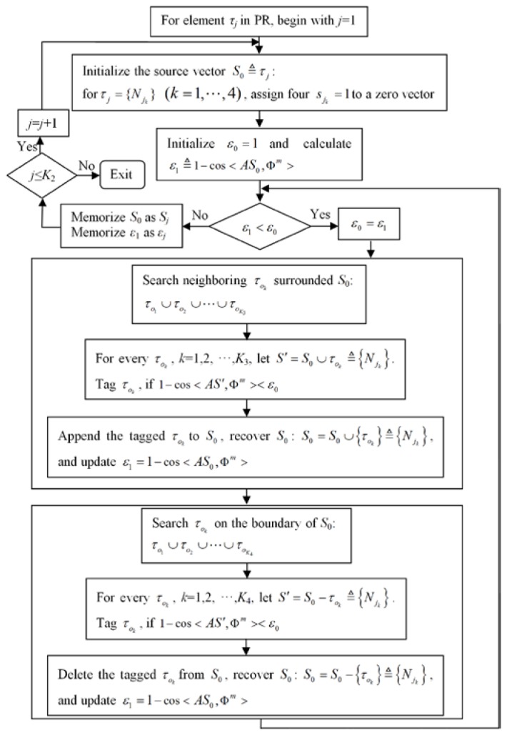
Flowchart of the region growing algorithm.
3.3 Probability reconstruction
Although the proposed optimal model (4) has the optimum solution, it might be non-robust. The solution might reject some true source nodes under a propagation error from a mesh split error, measurement error, or other type of error. Because certain types of errors are unavoidable, a probability model was developed to describe the reconstructed source distribution with a reflection of the error certainty.
After using the region growing method in the PR, an error sequence was obtained. If error is considerably large, the corresponding grown source is rejected. On the other hand, if both and are sufficiently small and are approximately equal, we cannot reject the hypothesis that both and are sources, i.e., if we chose an optimal source tied with a minimum error, we have a significant risk of a false rejection. A false rejection is demonstrated in Section 4 and 5. Additionally, the remaining errors, denoted as set , must demonstrate a normal distribution (ND); otherwise, presents a systematic error rather than a random error. If does not show an ND, another subset with an ND is extracted.
To achieve this, is refined as , where is the significance level, and is an ND with parameters and evaluated from the sample mean and variance of . Given an , is determined by searching the parameters and so that obeys ND. A grown source set is chosen as , where is the conformance error determined by correspondingly. Then, at a discretized node , the probability that the node is a source node can be defined as
| (5) |
where is the number of occurrences of in , i.e., , if a such that .
Let be the value of the assumed uniform photon density of the actual source, represents an event in which is a source node, and represents an event in which is not a source node. Then, the probability of node being a source node is represented as. The probability of all the element nodes being the light source, called the PS, can be defined as
| (6) |
The definition of in Eq. (5) implies an assumption that if node has the maximum number of occurrences, then there is a certain event in which is a source node, i.e., . The expectation of at node can be expressed as . In this way, the PS offers a probability distribution of the nodes in the PR being the light source. Statistically, the average photon density distribution (APDD) can be represented as , and .
4. Numerical experiments
In the experiments, we compared the results between hp-FEM [21,34] and the proposed probability method. Both a distance error and a conformance error were employed for the error assessment. The distance error was defined as the distance between the true source center and the reconstructed source center [21]. The conformance error is defined as , where and represent the CSPD resulting from the reconstructed source and the MSPD respectively. In our method, the reconstructed source center is defined as the probability core, which has the greatest probability, while the conformance error is defined as , which results from the APDD.
In numerical simulations, a heterogeneous cylindrical phantom of 30 mm in height and 10 mm in radius was applied to model as a mouse chest. The phantom consisted of five types of materials to represent the adipose, lungs, liver, heart, and bone (Fig. 3(a)). In this paper, we only described a single-source simulation, as shown in Fig. 3(a). The source was a solid sphere with a 1 mm radius with a uniform photon density of 0.238 nW/mm3 centered at (3,5,0) inside the right lung (Fig. 3(a)). The optical parameters listed in Table 1 were set the same as those in [34], which were supported by Prof. Ge Wang's lab (Bioluminescence Tomography Laboratory, Department of Radiology, University of Iowa). The measured surface data were obtained using a modified molecular optical simulation environment (MOSE), as shown in Fig. 3(b). In this paper, only the data on the cylinder side were used for the reconstruction.
Fig. 3.
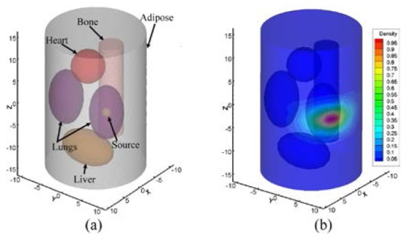
Heterogeneous phantom. (a) with a single-source in the right lung. (b) measured surface photon density (MSPD) distribution after normalization.
The phantom was discretized into 3,937 nodes including 1,298 side surface nodes. The volume of the cylinder was divided into 17,882 tetrahedrons tagged with the corresponding organ codes.
4.1 Robustness of rough positioning
We next investigated the robustness of the location. There are a number of factors affecting the robustness. However, for rough positioning, there are two main contributing factors, i.e., the threshold and the ROI, where is used to extract the reconstructed elements. To test the robustness of our method and hp-FEM with regards to , as shown in Fig. 4, eight experiments with were performed respectively, where the ROI of the probability method was cropped between −3 and 3 along the z-axis; the PR of hp-FEM was a cylindrical region confined in a box region . The results of the probability method (Fig. 4(a)) showed that a minimum conformance error was achieved in the right lung when , i.e., the source was pinpointed correctly when . However, for hp-FEM false positioning was unavoidable when , and the source was pinpointed correctly only when (Fig. 4(b)). Compared with hp-FEM, the probability method was more robust against .
Fig. 4.

The robustness with regards to . (a) conformance error of the probability method as a function of , where the cropped interval of the ROI was . (b) distance error of hp-FEM as a function of , where the PR was bounded in a box region .
At a fixed for different ROIs, every organ region bounded in the ROIs was supposed to be a PR. To avoid infinitely many solutions and guarantee a containment of the measured data region on the surface, six ROIs were tested in the numerical experiments, and the resulting conformance errors are shown in Table 2. For each column, the right lung featured the minimum error, which showed that rough positioning was robust to positioning the right organ with respect to the ROI. For hp-FEM, the PR is another factor contributing to the robustness. To test the robustness with regards to the PR, let and be the interval [-10,10], the distance errors together with the positioned organs are shown in Table 3 under different ... Although there were five occasions when the reconstructed source was located in the right lung, the false positioning was unavoidable when the PR was chosen as . For hp-FEM, a priori PR may be indispensable to obtain an accurate reconstruction [34]. Compared with hp-FEM, the probability method was more robust against the cropped interval.
Table 2. Conformance errors of the probability method to the cropped interval of the ROI when β = 0.9. CI stands for the cropped interval.
| CI (mm) | [-4,5] | [-3,5] | [-2,5] | [-3,3] | [-3,4] | [-5,4] |
|---|---|---|---|---|---|---|
| Adipose | 0.164 | 0.164 | 0.164 | 0.164 | 0.164 | 0.164 |
| Right lung | 0.097 | 0.097 | 0.097 | 0.097 | 0.097 | 0.097 |
| Left lung | 0.811 | 0.811 | 0.811 | 0.811 | 0.811 | 0.811 |
| Bone | 0.866 | 0.866 | 0.866 | 0.866 | 0.866 | 0.866 |
Table 3. Distance errors of hp-FEM to the PR when β = 0.9. The PR of hp-FEM is a cylindrical region confined in a box region , where and are the interval [-10,10].
| Iz (mm) | [-4,5] | [-3,5] | [-2,5] | [-3,3] | [-3,4] | [-5,4] |
|---|---|---|---|---|---|---|
| Adipose | 3.501 | |||||
| Right lung | 2.482 | 2.482 | 2.482 | 2.482 | 2.482 |
4.2 Uncertainty of the growing method
As mentioned earlier, the region growing method was implemented to solve the proposed optimization problem. After cropping the ROI in interval along the z-axis and choosing , the PR, which was discretized to 138 nodes and 359 tetrahedrons, was positioned in the right lung of the ROI. After running through the tetrahedrons in the PR to grow the sources, 359 sources were obtained. We illustrated four such sources in Figs. 5(a)-5(d). Figure 5(e) shows the normalized MSPD. Correspondingly, the normalized CSPDs calculated by the four grown sources of Figs. 5(a)-5(d) are visualized in Figs. 5(f)-5(i). Figure 5(i) has the lowest similarity compared with Fig. 5(e) among Figs. 5(f)-5(i). A closer evaluation revealed that the conformance errors between Figs. 5(f)-5(i) and Fig. 5(e) were , , , and respectively. It can be deduced that the objective assessment is in accord with the subjective assessment. This experiment suggested that if a conformance error was relatively considerably large, the corresponding source should be rejected.
Fig. 5.
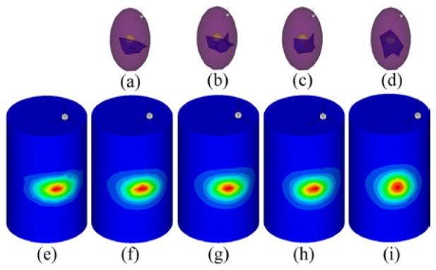
Four results of region growth. The sub-images (a)-(d) on the first line are the grown sources in the right lung. (e) is the original MSPD after normalization. Correspondingly, the sub-images (f)-(i) are the normalized CSPD resulting from (a)-(d).
The conformance error can be used to evaluate the quantitative assessment. However, the slight differences in errors may not be statistically significant. When the type of error, such as a measurement error, is changed slightly, the priority order of the quantitative error may also change. Our work shows the uncertainty of the source under a measurement error. A measurement error is mainly generated by using a charge coupled device (CCD) camera and post-processing operations, such as mapping the gray-level values in the images into energy values or using MOSE to obtain the measured surface data. To demonstrate the impact of the post-processing step with respect to the energy quantization error, a random noise valued in was added into the pseudo-color region of Fig. 5(e), where was the maximum value of MSPD after normalization. Figures 6(a) and 6(b) show the optimum sources when the noise was not or was added respectively. The sources were grown from two different seed tetrahedrons. The conformance error resulted in the sources of Fig. 6(a) and Fig. 6(b) being and respectively. After noise was added, the conformance error was reduced from to , whereas the composed elements increased in number from 15 to 32. The noise simulates a post-processing error. Owing to the uncertainty of the error, we were unable to determine which source in Fig. 6 was the looking for true source. If we consider only the blue elements in Fig. 6(a) as the true source, we will reject the other seventeen blue elements in Fig. 6(b), i.e., a false rejection has taken place. The noise experiment demonstrates that the sources tied with the small errors of the error sequence might all be accepted as true sources.
Fig. 6.

Reconstructed optimum sources when a noise is not or is added to the MSPD. (a) reconstructed optimum source composed of fifteen tetrahedrons without noise. (b) reconstructed optimum source, which is composed of 32 tetrahedrons when 5% random noise was added.
4.3 Accuracy and reasonableness of the probability reconstruction
To decrease the risk of a false rejection, we developed a probability model in this work. The conformance error sequence memorized during the region growth is plotted in Fig. 7(a). In the numerical studies, let and be 0.05 and the first 50% critical number of respectively. was determined in a search manner. When be , , which is accumulated between and in Fig. 7(a), was specified to be within the range of . The sample mean and variance of the 45 accumulated elements of were and respectively. Consequently, was obtained including 53 elements of . The sequence passed a normality test, i.e., . The histogram of sequence is shown in Fig. 7(b).
Fig. 7.

Extraction of the conformance errors during probability reconstruction. (a) visualization of the conformance error sequence , where the horizontal axis represents the subscript of , the vertical axis shows the values of , and the data between and constitute . (b) error histogram of data and .
Based on Eq. (6), the PS was conducted from 53 accepted errors. The reconstructed PS and hp-FEM results are shown in Figs. 8 and 9 respectively for comparison. In order to present more accurate results, when hp-FEM was used, the parameters and were chosen as and 0.95 respectively. The reconstructed PS (Figs. 8(a) or 8(b)) consisted of 64 different nodes discretized from the right lung. The conformance error of our method was , which was demonstrated by the similarity between Figs. 8(c) and 5(e). However, the conformance error of hp-FEM was , which was demonstrated by the difference between Fig. 9(a) and Fig. 5(e). Figures 8(d)-8(f) show slices along the axes at the PS core mm. Because the geometrical center of the actual source was located at mm, the distance error of the proposed method was thus 1.8 mm, whereas the center of hp-FEM of the reconstructed source was mm, and the distance error was 1.96 mm (Fig. 9(b)). The distance error of hp-FEM was inferior to our method. Both the conformance error and the distance error showed that the accuracy of our proposed probability method was superior to hp-FEM.
Fig. 8.
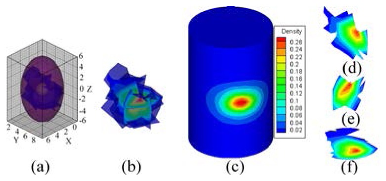
Reconstructed results of the probability method, where , and the ROI is cropped in along the z-axis. (a), (b) are the reconstructed PS. (c) normalized surface photon density calculated using APDD. (d)-(f) are the slices, which are perpendicular to the x, y, and z-axes at the probability core mm respectively.
Fig. 9.
Reconstructed results of hp-FEM, where , and the PR is the region bounded in . (a) normalized surface photon density calculated using the reconstructed sources. (b) reconstructed source with a distance error of 1.96 mm. (c) enlarged source, where the normalized photon density is dyed with a pseudo-color after interpolation.
For hp-FEM, the maximum value of the reconstructed photon density was more than ten-times greater than its minimum value (Fig. 9(c)). However, for our method, the source was constrained by a uniform distribution in model (4). The PS simply represented a probability distribution, and the photon density was represented by APDD based on average statistics. This suggests that model (4) and the PS delivered more reasonable results.
4.4 Reconstruction efficiency
To evaluate the reconstruction efficiency of the proposed probability method, we also compared it with hp-FEM. The experiments were implemented using Matlab code on a PC powered by Intel Duo CPU E6550 (2.33GHz) processors with 2 GB of RAM. It took hp-FEM 11.2 min to finish the regularization, and a total of 13.6 min to finish the whole process. In comparison, it took the probability method 5.6 min and 2.2 min for rough positioning and region growth respectively. The total time taken for the probability method was approximately 8.3 min. The efficiency of the probability method was mainly determined by the regularization during the rough positioning and the time spent on region growth.
5. In vivo experiments
Since the uptake of I-131 mainly occurs in the bladder and thyroid [21] in the in vivo experiments, we would reconstruct the bladder and thyroid in succession to show the reconstruction of the deep and subcutaneous targets respectively. The in vivo experimental data were provided by Hu et. al [21], in which the experimental data used for the reconstruction of the bladder and thyroid were acquired 2 hours and 24 hours later after the intravenous tail injection respectively. The injected doses of I-131 were 400 and 450 μCi respectively. The optical parameters of the biological tissues listed in Table 4 were set the same as those in [21].
Table 4. Optical parameters of the biological tissues, where is the reducing scattering coefficient.
| Material | Adipose/ Bladder |
Heart | Lungs | Liver/ Spleen |
Stomach | Kidneys | Bone | Intestines |
|---|---|---|---|---|---|---|---|---|
| 0.1017 | 1.5477 | 4.6832 | 9.2860 | 0.3082 | 1.7334 | 1.5233 | 0.2891 | |
| 1.2929 | 1.1674 | 2.3271 | 0.7786 | 1.6320 | 2.7599 | 3.0393 | 1.3548 |
5.1 Reconstruction of the bladder
In order to reconstruct the bladder conveniently, we cropped the torso data of the whole mouse so that the interception excluded the thyroid data. Confined to the reduced torso data, we assumed that the uptake of I-131 only occurred in the bladder. After the interception of the torso, the mouse was discretized into 3,718 nodes including 1,035 surface nodes (Fig. 1(a1)). The volume of the mouse was split into 18,952 tetrahedrons.
5.1.1 Robustness of the rough positioning
Figure 1(a) illustrates the rough positioning after MOSE was used to obtain the synthetic data. The robustness experiments with regards to are shown in Fig. 10. The ROI of our method was cropped between 0 and 7 along the z-axis. The PR of hp-FEM was bounded in a box region . In accordance with the numerical studies, the in vivo results showed that a minimum conformance error was achieved in the bladder when , i.e., the source was pinpointed correctly when (Fig. 10(a)). However, for hp-FEM, the sources were all pinpointed falsely within the adipose (Fig. 10(b)). Compared with hp-FEM, the probability method is more robust against .
Fig. 10.
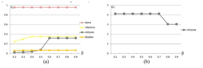
The robustness with regards to . (a) conformance error of the probability method as a function of , where the cropped interval of the ROI is . (b) distance error of hp-FEM as a function of , where the PR is a box region .
Let . Table 5 shows the conformance errors of the positioning for different ROIs. For every column, the bladder features the minimum error, which shows that the rough positioning was also robust with respect to the ROI in the in vivo experiments. At the fixed and for different , the distance errors of hp-FEM together with the positioned organs are shown in Table 6. Although on one occasion the reconstructed source was located in the bladder with a minimum error of 1.43 mm, hence the true position of the source center showed a large amount of randomness. More often, the source center was positioned within the adipose, and the positioning was untrue. Compared with hp-FEM, our probability method was more robust against the ROI in the bladder reconstruction.
Table 5. Conformance errors of the probability method for the cropped interval of the ROI when β = 0.9. CI stands for a cropped interval.
| CI (mm) | [0,5] | [0,6] | [0,7] | [0,8] | [1,8] | [2,8] | [3,8] |
|---|---|---|---|---|---|---|---|
| Bladder | 0.07 | 0.07 | 0.07 | 0.07 | 0.07 | 0.07 | 0.07 |
| Apose | 0.32 | 0.32 | 0.32 | 0.32 | 0.32 | 0.32 | 0.32 |
| Intestines | 0.38 | 0.34 | 0.35 | 0.35 | 0.35 | 0.35 | 0.35 |
| Bone | 0.96 | 0.96 | 0.96 | 0.96 | 0.96 | 0.96 | 0.96 |
Table 6. Distance error of hp-FEM for the PR when β = 0.9. The PR of hp-FEM is bounded in a box region , where and are the interval [0,40] and [0,30] respectively.
| Iz (mm) | [0,5] | [0,6] | [0,7] | [0,8] | [1,8] | [2,8] | [3,8] |
|---|---|---|---|---|---|---|---|
| Bladder | 1.43 | ||||||
| Adipose | 3.19 | 3.84 | 3.03 | 3.03 | 3.03 | 2.95 |
5.1.2 Uncertainty of the growing method
In the studies of the reconstruction of the bladder, after choosing as 0.9 and confining the ROI in the cropped interval , the source was located in the bladder qualitatively (Fig. 1(a4)) by assuming every organ (Fig. 1(a3)) in the ROI (Fig. 1(a2)) was the PR. The PR was the whole bladder (Fig. 1(a4)), which was discretized to 73 nodes and 203 tetrahedrons. After using the region growing method shown in Fig. 2, 203 sources were obtained. We illustrated four of these sources in Figs. 1(b1)-1(b4). Correspondingly, the normalized CSPDs are visualized in Figs. 1(b5)-1(b8). Figure 1(b9) shows the normalized MSPD. The figure also indicates that the similarity between Fig. 1(b8) and Fig. 1(b9) is clearly low, and Figs. 1(b5)-1(b7) are similar with Fig. 1(b9). The conformance errors between Figs. 1(b5)-1(b8) and Fig. 1(b9) are 0.0486, 0.0510, 0.0511, and 0.4468 respectively. Bearing in mind the objective and subjective assessments, the source of Fig. 1(b4) was rejected. This demonstrates that if the conformance errors of the sequence resulting from the region growth are sufficiently large, they should be rejected.
To demonstrate the impact of the post-processing step with respect to the energy quantization error, similar with the numerical studies, random noise valued at was added into the pseudo-color region of Fig. 1(b9), where was similarly valued. Figure 11(a) shows two reconstructed optimum sources, which also are shown in Figs. 11(b) and 11(c) when the noise was and was not added respectively. Figures 11(a) and 11(c) show a false rejection where three additional elements were rejected when no noise was added. The noise experiment also demonstrated the uncertainty of the growing method.
Fig. 11.
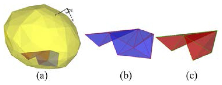
Reconstructed optimum sources when noise was or was not added to the MSPD. (a) two reconstructed sources. (b) reconstructed optimum source composed of five tetrahedrons, when 5% random noise was added. (c) reconstructed optimum source composed of two tetrahedrons without noise.
5.1.3 Accuracy and reasonableness of the probability reconstruction
We plotted the conformance error sequence in Fig. 12(a). In the in vivo experiments of the bladder reconstruction, and were valued the same as those in the numerical experiments. When , was specified within the range of between and (Fig. 12(a)), and the element number of was 84. Correspondingly, and . Consequently, we obtained the ND sequence , where including 81 elements of . The histogram of sequence is shown in Fig. 12(b), where .
Fig. 12.

Extraction of conformance errors during probability reconstruction. (a) visualization of the conformance error sequence , where the horizontal axis represents the subscript of , and the vertical axis shows the values of . The data between and constitute . (b) error histogram of data , where .
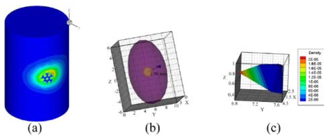
The reconstructed PS and the result of hp-FEM are shown in Figs. 13 and 14 respectively for comparison. The PR and value of hp-FEM were chosen as and 0.9 respectively. The PS was conducted from 81 accepted sources and consisted of 53 different nodes (Figs. 13(a) and 13(b)). The conformance error of the PS was . The error showed that the distributions of the CSPD (Fig. 13(c)) and MSPD (Fig. 1(b9)) were considerably close. However, the result of hp-FEM (Fig. 14(a)) and the measured distribution shown in Fig. 1(b9) were significantly different (with a conformance error of 0.433). Figures 13(d)-13(f) show slices along the axes of the PS core mm. Because the geometrical center of the bladder was obtained from micro-CT images at mm, the distance error of the PS was thus 1.08 mm. However, the distance error of hp-FEM was 1.43 mm (Fig. 14(b)) [21]. Both the conformance error and the distance error indicated that the accuracy of our method was superior to hp-FEM in the in vivo experiments.
Fig. 13.

Reconstructed results of the probability method, where , and the ROI is cropped in along the z-axis. (a) and (b) are the reconstructed PS. (c) normalized surface photon density calculated by APDD. (d)-(f) are the slices perpendicular to the x, y, z-axes at the probability core of mm respectively.
Fig. 14.
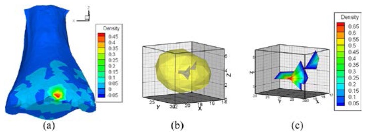
Reconstructed results of hp-FEM, where , and the PR is the region bounded in the region . (a) normalized surface photon density calculated from the reconstructed sources. (b) reconstructed source. (c) enlarged source, where the photon density is dyed with a pseudo-color after interpolation.
For hp-FEM, the maximum energy value of the reconstructed source density was also more than ten-times greater than its minimum value (Fig. 14(c)). This also suggested that the PS delivered more reasonable results.
5.1.4 Efficiency
We also compared the probability method with hp-FEM to evaluate the efficiency of the in vivo experiments. It took hp-FEM 4.0 min to finish the regularization. The time cost of the whole process was 6.7 min. In comparison, it took the probability method 4.0 min and 0.4 min for rough positioning and region growth respectively. The total time cost for the probability method was approximately 5.9 min.
5.2 Reconstruction of the thyroid
In the studies of the reconstruction of the thyroid, the mouse was discretized into 4,740 nodes including 1,820 surface nodes. The volume of the mouse was split into 22,072 tetrahedrons.
5.2.1 Robustness of the rough positioning
Since the thyroid was not identified via micro-CT anatomically, the distance error could not be obtained spatially. We did not compare the robustness between the hp-FEM and the probability method in this subsection.
To test the robustness of our method with regards to , eight experiments with were performed (Fig. 15). The in vivo results showed that the source was pinpointed correctly when .
Fig. 15.
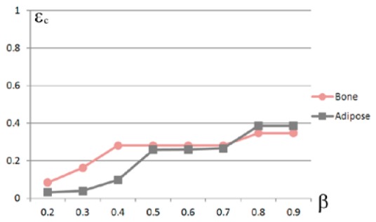
Conformance errors for vs. values showing the robustness of , where the ROI is confined in the cropping interval .
Let , Table 7 shows the conformance errors of the positioning for different ROIs. For every column, the thyroid features the minimum error, which shows that the rough positioning was robust with respect to the cropped interval.
Table 7. Conformance errors of the probability method for the cropped interval of the ROI when β = 0.7. CI stands for a cropped interval.
| CI (mm) | [18,28] | [22,28] | [20,28] | [22,30] | [20,30] | [18,30] | [18,28] |
|---|---|---|---|---|---|---|---|
| Adipose | 0.26 | 0.26 | 0.26 | 0.26 | 0.26 | 0.26 | 0.26 |
| Bone | 0.28 | 0.28 | 0.28 | 0.28 | 0.28 | 0.28 | 0.28 |
5.2.2 Uncertainty of the growing method
In the studies of the reconstruction of the thyroid, after choosing as 0.7 and confining the ROI in the cropped interval , the source was located in the adipose qualitatively. The PR(adipose) was discretized into 3108 elements. After using the region growing method, a conformance error sequence corresponding to 3108 sources was obtained.
Of course, there was an optimum source with a minimum error in . However, maybe it is not a certain event that the source is only composed of the elements from the optimum source. To demonstrate the uncertainty of the source reconstruction, random noise valued at was added into the measured surface density, where was the maximum value of MSPD after normalization. Three reconstructed results are shown in Fig. 16. Figure 16(a) shows the optimum sources when no noise was added. Figures 16(b) and 16(c) are two different optimum sources after adding two different 5% random noise respectively. The conformance errors of the three reconstructions were 0.04760, 0.04713 and 0.05283 respectively. The conformance error decreased slightly in Fig. 16(b). On the contrary, the error increased in Fig. 16(c). It can be seen that the conformance error was increased or decreased randomly after adding random noise. Therefore, the optimum source was sensitive under the perturbation of the noise. For any optimum source, it might reject some other real source elements. The reconstruction of the thyroid also demonstrated the uncertainty of the growing source .
Fig. 16.
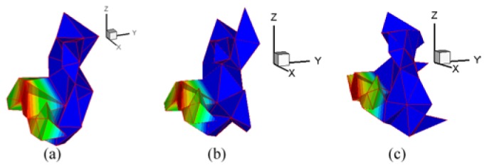
Reconstructed optimum sources when noise was or was not added to MSPD. (a) reconstructed optimum source composed of 49 tetrahedrons without noise. (b) and (c) are the two optimum sources composed of 60 and 76 tetrahedrons respectively, when two different 5% random noise were added.
5.2.3 Accuracy and reasonableness of the probability reconstruction
There were 2433 large errors reaching the condition in the error sequence . They were sufficiently large, and should be rejected. Confining to the remaining 675 errors are shown in Fig. 17(a). In the in vivo experiments of the thyroid, let be 0.05, be the first 50% critical number of . When , was specified within the range of between and (Fig. 17(a)), and the element number of was 514. Correspondingly, and . Consequently, the ND sequence was obtained, where including 504 elements of . The histogram of sequence of is shown in Fig. 17(b), where .
Fig. 17.

Extraction of conformance errors during probability reconstruction. (a) visualization of the conformance error sequence , where the horizontal axis represents the subscript of , and the vertical axis shows the values of . The data between and constitute . (b) error histogram of data , where .
The reconstructed PS and the result of hp-FEM are shown in Figs. 18 and 19 respectively. The PR and the parameter of hp-FEM were chosen as and 0.7 respectively. Although both locations of the reconstructed sources were positioned in the adipose (shown in Figs. 18(a), 18(b), 19(a) and 19(b)), the conformance error indicated that the accuracy of our method was superior to hp-FEM in the in vivo experiments of the thyroid. The conformance error of the PS was . The error demonstrated that the distributions between the MSPD (Fig. 18(c)) and CSPD (Fig. 18(d)) were close. Figure 18(e) shows the reconstructed PS. Figures 18(f)-18(h) show the slices along the axes of the PS core. It can be seen that the reconstructed source was a subcutaneous target. However, for hp-FEM, the maximum and minimum density values after normalization indicated by the color-bar in Fig. 19(c) were 0.45 and 0.05 respectively. Compared with the corresponding values in Fig. 18(d), they were more different from those in Fig. 18(c). The differences were demonstrated by the conformance error. The conformance error between the normalized surface density of hp-FEM (Fig. 19(c)) and the measured distribution shown in Fig. 18(c) was 0.200.
Fig. 18.

Reconstructed results of the probability method, where , and the ROI is cropped in [22,28] along the z-axis. (a) and (b) are the front and side perspective views of the source, which is dyed in blue. (c) original MSPD after normalization. (d) normalized surface photon density calculated by APDD. (e) is the reconstructed PS. (f)-(h) are the slices perpendicular to the x, y, z-axes at the probability core of respectively.
Fig. 19.

Reconstructed results of hp-FEM, where , and the PR is the region bounded in . (a) and (b) are the front and side perspective views of the source, which is dyed in blue. (c) normalized surface photon density calculated from the reconstructed sources. (d) is the reconstructed source.
For hp-FEM, the maximum energy value of the reconstructed source density was also more than ten-times greater than its minimum value (Fig. 19(d)). This also suggested that the PS delivered more reasonable results.
5.2.4 Efficiency
We also compared the probability method with hp-FEM to evaluate the efficiency of the reconstruction of the subcutaneous target. The time cost of the whole process for hp-FEM was 11.7 min. In comparison, it took the probability method 1.1 min and 43.7 min for rough positioning and region growth respectively. The total time cost for the probability method was approximately 45 min.
6. Discussion and conclusions
It is worth pointing out that rough positioning is very important in the proposed probability method. In the experiments of the bladder, when we took the entire ROI as the PR and performed the region growing method there, the resulting reconstructed source was changed from the bladder to adipose. In practical terms, a large PR may cause a surface deviation, as in [21–23] and [34]. Actually, if the node number of the discrete PR is greater than the node number on the surface, there are infinitely many solutions for Eq. (1), and the error is out of control. In this work, the PR was assumed to be an organ confined in the ROI, which effectively improved the ill-posed aspect of Eq. (1).
The homogeneous hypothesis is reasonable. The probability model was based upon the characteristic of the homogeneity in an organ. Although for the sake of convenience the homogeneity was only an approximation assumption, the uptake of the implant source and the bladder was homogeneous in this paper. As an additional example, the uptake of a tumor is usually homogeneous because a tumor comprises of the same tumor cells. The proposed technique may be extended to self-luminescence tomography, such as BLT, after the homogeneous hypothesis. However, in general, the excited diffuse model, such as fluorescence molecular tomography (FMT), does not satisfy the homogeneous hypothesis. Therefore, the method may not be directly extended to excited luminescence tomography.
The space constraints involved in Eq. (4) are necessary. The important aspect of the region growing method is to transform an inverse problem into a forward problem by searching for the local optimum solution under two constraints. The growing scheme is by nature tied with a space constraint (condition 2) to ensure that there are no isolated source points. However, the TR method, which was used in [21–23] and [34], had nothing to do with space constraint, and it may be unreasonable. The FEM can convert a discrete result into a continuous result through interpolation, and any point in an element is interpolated by the elemental nodes. If there is an isolated source node, there is no way to identify how to deal with the points surrounding it.
The optimization model (4) is reasonable. The reconstructed source of hp-FEM, as shown in Figs. 9(c), 14(c) and 19(d), was unreasonable because the reconstructed maximum energy value was more than ten-times greater than the minimum value. An organ may comprise certain stem organs. However, the stem organs should not be significantly different in terms of the reconstructed energy value. This unreasonableness was not present in the optimization model (4) because the source density was constrained with a uniform distribution.
It should be pointed out that the region growing method suffers from several limitations in terms of solving the optimization. Some new techniques are expected to be designed to solve the optimization directly. Because a growth begins with one element and the results cannot be extended to another isolated region topologically, the method is unable to deal with multiple sources directly. When the method deals with multiple targets, this shortcoming can be partially overcome using two steps. First, divide an entire body region into multiple sub-regions so that each sub-region contains only one source. Second, implement the method repeatedly for each sub-region. As another shortcoming, the method does not reconstruct the source density or APDD, because the value of the assumed uniform photon density is usually unknown. Fortunately, quantitative detection generally focuses on detecting the position of the tumor, and the source location is more important than the source intensity for source reconstruction.
For the reconstruction efficiency, the computation of the proposed method mainly depends on source positioning and region growing. If the fineness of the mesh is doubled, the computation of the region growing would be doubled too. However, the computational cost of our method could be reduced after ignoring invalid growth since the sources delivering large conformance errors were rejected, e.g., the computational time of the region growing was reduced from 43.7 min to 6.5 min in the reconstruction of the thyroid after using the ‘continue’ statement in the program. In detail, the technique prevented elements, which delivered conformance errors of greater than 0.5, to be seed elements. Therefore, the subsequent growth process was reduced. This implies that our method may be more efficient than hp-FEM after necessary program optimization.
In this paper, we proposed an optimization using two constraints to model the CLT inverse problem. We also developed a probabilistic assessment method for CLT reconstruction that was able to determine with probability whether an organ node was a source node. The reconstruction results were more reasonable because our method took into account homogeneous uptakes for homogeneous organs. Comparative experimental results demonstrated that our method was able to achieve a robust, accurate, and reasonable result.
Acknowledgments
This paper was supported by the National Natural Science Foundation of China under Grant No. 61370050, 61302024, the National Basic Research Program of China (973 Program) under Grant No. 2011CB707700, and the Early Career Development Award of SKLMCCS (Y3S9021F2B). The authors would like to thank Adjunct Assistant Professor Dr. Karen M. von Deneen from the University of Florida and Dr. Ji Zhang from the University of Southern Queensland, Australia for their help in modifying this paper.
References and links
- 1.Pysz M. A., Gambhir S. S., Willmann J. K., “Molecular imaging: current status and emerging strategies,” Clin. Radiol. 65(7), 500–516 (2010). 10.1016/j.crad.2010.03.011 [DOI] [PMC free article] [PubMed] [Google Scholar]
- 2.Mankoff D. A., “A definition of molecular imaging,” J. Nucl. Med. 48(6), 18N–21N (2007). [PubMed] [Google Scholar]
- 3.Massoud T. F., Gambhir S. S., “Molecular imaging in living subjects: seeing fundamental biological processes in a new light,” Genes Dev. 17(5), 545–580 (2003). 10.1101/gad.1047403 [DOI] [PubMed] [Google Scholar]
- 4.Ntziachristos V., Ripoll J., Wang L. V., Weissleder R., “Looking and listening to light: the evolution of whole-body photonic imaging,” Nat. Biotechnol. 23(3), 313–320 (2005). 10.1038/nbt1074 [DOI] [PubMed] [Google Scholar]
- 5.Cho J. S., Taschereau R., Olma S., Liu K., Chen Y. C., Shen C. K., van Dam R. M., Chatziioannou A. F., “Cerenkov radiation imaging as a method for quantitative measurements of beta particles in a microfluidic chip,” Phys. Med. Biol. 54(22), 6757–6771 (2009). 10.1088/0031-9155/54/22/001 [DOI] [PMC free article] [PubMed] [Google Scholar]
- 6.Robertson R., Germanos M. S., Li C., Mitchell G. S., Cherry S. R., Silva M. D., “Optical imaging of Cerenkov light generation from positron-emitting radiotracers,” Phys. Med. Biol. 54(16), N355–N365 (2009). 10.1088/0031-9155/54/16/N01 [DOI] [PMC free article] [PubMed] [Google Scholar]
- 7.Ruggiero A., Holland J. P., Lewis J. S., Grimm J., “Cerenkov luminescence imaging of medical isotopes,” J. Nucl. Med. 51(7), 1123–1130 (2010). 10.2967/jnumed.110.076521 [DOI] [PMC free article] [PubMed] [Google Scholar]
- 8.Beattie B. J., Thorek D. L. J., Schmidtlein C. R., Pentlow K. S., Humm J. L., Hielscher A. H., “Quantitative modeling of Cerenkov light production efficiency from medical radionuclides,” PLoS ONE 7(2), e31402 (2012). 10.1371/journal.pone.0031402 [DOI] [PMC free article] [PubMed] [Google Scholar]
- 9.Liu H., Ren G., Miao Z., Zhang X., Tang X., Han P., Gambhir S. S., Cheng Z., “Molecular optical imaging with radioactive probes,” PLoS ONE 5(3), e9470 (2010). 10.1371/journal.pone.0009470 [DOI] [PMC free article] [PubMed] [Google Scholar]
- 10.Boschi F., Calderan L., D’Ambrosio D., Marengo M., Fenzi A., Calandrino R., Sbarbati A., Spinelli A. E., “In vivo 18F-FDG tumour uptake measurements in small animals using Cerenkov radiation,” Eur. J. Nucl. Med. Mol. Imaging 38(1), 120–127 (2011). 10.1007/s00259-010-1630-y [DOI] [PubMed] [Google Scholar]
- 11.Robertson R., Germanos M. S., Manfredi M. G., Smith P. G., Silva M. D., “Multimodal imaging with (18)F-FDG PET and Cerenkov luminescence imaging after MLN4924 treatment in a human lymphoma xenograft model,” J. Nucl. Med. 52(11), 1764–1769 (2011). 10.2967/jnumed.111.091710 [DOI] [PubMed] [Google Scholar]
- 12.Xu Y., Chang E., Liu H., Jiang H., Gambhir S. S., Cheng Z., “Proof-of-concept study of monitoring cancer drug therapy with Cerenkov luminescence imaging,” J. Nucl. Med. 53(2), 312–317 (2012). 10.2967/jnumed.111.094623 [DOI] [PMC free article] [PubMed] [Google Scholar]
- 13.Park J. C., Il An G., Park S. I., Oh J., Kim H. J., Su Ha Y., Wang E. K., Min Kim K., Kim J. Y., Lee J., Welch M. J., Yoo J., “Luminescence imaging using radionuclides: a potential application in molecular imaging,” Nucl. Med. Biol. 38(3), 321–329 (2011). 10.1016/j.nucmedbio.2010.09.003 [DOI] [PubMed] [Google Scholar]
- 14.Holland J. P., Normand G., Ruggiero A., Lewis J. S., Grimm J., “Intraoperative imaging of positron emission tomographic radiotracers using Cerenkov luminescence emissions,” Mol. Imaging 10(3), 177–186 (2011). [PMC free article] [PubMed] [Google Scholar]
- 15.Mitchell G. S., “In vivo Cerenkov luminescence imaging: a new tool for molecular imaging,” Phil. Trans. R. Soc. A 369, 4605–4619 (2011). [DOI] [PMC free article] [PubMed] [Google Scholar]
- 16.Spinelli A. E., D’Ambrosio D., Calderan L., Marengo M., Sbarbati A., Boschi F., “Cerenkov radiation allows in vivo optical imaging of positron emitting radiotracers,” Phys. Med. Biol. 55(2), 483–495 (2010). 10.1088/0031-9155/55/2/010 [DOI] [PubMed] [Google Scholar]
- 17.Thorek D. Lj., Robertson R., Bacchus W. A., Hahn J., Rothberg J., Beattie B. J., Grimm J., “Cerenkov imaging - a new modality for molecular imaging,” Am J Nucl Med Mol Imaging 2(2), 163–173 (2012). [PMC free article] [PubMed] [Google Scholar]
- 18.Li C., Mitchell G. S., Cherry S. R., “Cerenkov luminescence tomography for small-animal imaging,” Opt. Lett. 35(7), 1109–1111 (2010). 10.1364/OL.35.001109 [DOI] [PMC free article] [PubMed] [Google Scholar]
- 19.Spinelli A. E., Kuo C., Rice B. W., Calandrino R., Marzola P., Sbarbati A., Boschi F., “Multispectral Cerenkov luminescence tomography for small animal optical imaging,” Opt. Express 19(13), 12605–12618 (2011), http://www.opticsinfobase.org/oe/fulltext.cfm?uri=oe-19-13-12605&id=218880 10.1364/OE.19.012605 [DOI] [PubMed] [Google Scholar]
- 20.Hu Z., Liang J., Yang W., Fan W., Li C., Ma X., Chen X., Ma X., Li X., Qu X., Wang J., Cao F., Tian J., “Experimental Cerenkov luminescence tomography of the mouse model with SPECT imaging validation,” Opt. Express 18(24), 24441–24450 (2010), http://www.opticsinfobase.org/oe/abstract.cfm?uri=oe-18-24-24441 10.1364/OE.18.024441 [DOI] [PubMed] [Google Scholar]
- 21.Hu Z., Ma X., Qu X., Yang W., Liang J., Wang J., Tian J., “Three-dimensional noninvasive monitoring iodine-131 uptake in the thyroid using a modified Cerenkov luminescence tomography approach,” PLoS ONE 7(5), e37623 (2012). 10.1371/journal.pone.0037623 [DOI] [PMC free article] [PubMed] [Google Scholar]
- 22.Hu Z., Chen X., Liang J., Qu X., Chen D., Yang W., Wang J., Cao F., Tian J., “Single photon emission computed tomography-guided Cerenkov luminescence tomography,” J. Appl. Phys. 112(2), 024703 (2012). 10.1063/1.4739266 [DOI] [Google Scholar]
- 23.Hu Z., Yang W., Ma X., Ma W., Qu X., Liang J., Wang J., Tian J., “Cerenkov luminescence tomography of aminopeptidase N (APN/CD13) expression in mice bearing HT1080 tumors,” Mol. Imaging 12(3), 173–181 (2013). [PubMed] [Google Scholar]
- 24.Zhong J., Tian J., Yang X., Qin C., “Whole-body Cerenkov luminescence tomography with the finite element SP3 method,” Ann. Biomed. Eng. 39(6), 1728–1735 (2011). 10.1007/s10439-011-0261-1 [DOI] [PubMed] [Google Scholar]
- 25.Zhang R., Davis S. C., Demers J. L. H., Glaser A. K., Gladstone D. J., Esipova T. V., Vinogradov S. A., Pogue B. W., “Oxygen tomography by Čerenkov-excited phosphorescence during external beam irradiation,” J. Biomed. Opt. 18(5), 050503 (2013). 10.1117/1.JBO.18.5.050503 [DOI] [PMC free article] [PubMed] [Google Scholar]
- 26.Demers J. L., Davis S. C., Zhang R., Gladstone D. J., Pogue B. W., “Čerenkov excited fluorescence tomography using external beam radiation,” Opt. Lett. 38(8), 1364–1366 (2013), http://www.opticsinfobase.org/vjbo/fulltext.cfm?uri=ol-38-8-1364&id=252787 10.1364/OL.38.001364 [DOI] [PMC free article] [PubMed] [Google Scholar]
- 27.Kojima F., Knopp J. S., “Inverse problem for electromagnetic propagation in a dielectric medium using Markov chain Monte Carlo method,” Int. J. Innov. Comput., Inf. Control 8(3), 2339–2346 (2012). [Google Scholar]
- 28.Aster R. C., Borchers B., Thurber C. H., Parameter estimation and inverse problems (2nd ed.) (Academic Press, Waltham, 2013). [Google Scholar]
- 29.Tropp J. A., Wright S. J., “Computational methods for sparse solution of linear inverse problems,” Proc. IEEE 98(6), 948–958 (2010). 10.1109/JPROC.2010.2044010 [DOI] [Google Scholar]
- 30.Ahn S., Chaudhari A. J., Darvas F., Bouman C. A., Leahy R. M., “Fast iterative image reconstruction methods for fully 3D multispectral bioluminescence tomography,” Phys. Med. Biol. 53(14), 3921–3942 (2008). 10.1088/0031-9155/53/14/013 [DOI] [PMC free article] [PubMed] [Google Scholar]
- 31.Kuo C., Coquoz O., Troy T. L., Xu H., Rice B. W., “Three-dimensional reconstruction of in vivo bioluminescent sources based on multispectral imaging,” J. Biomed. Opt. 12(2), 024007 (2007). 10.1117/1.2717898 [DOI] [PubMed] [Google Scholar]
- 32.Santosa F., “A level-set approach for inverse problems involving obstacles,” ESAIM Control Optim. Calc. Var. 1, 17–33 (1996). 10.1051/cocv:1996101 [DOI] [Google Scholar]
- 33.Aghasi A., Kilmer M., Miller E. L., “Parametric level set methods for inverse problems,” SIAM J. Imaging Sci. 4(2), 618–650 (2011). 10.1137/100800208 [DOI] [Google Scholar]
- 34.Han R., Liang J., Qu X., Hou Y., Ren N., Mao J., Tian J., “A source reconstruction algorithm based on adaptive hp-FEM for bioluminescence tomography,” Opt. Express 17(17), 14481–14494 (2009). 10.1364/OE.17.014481 [DOI] [PubMed] [Google Scholar]
- 35.Gao H., Zhao H., “Multilevel bioluminescence tomography based on radiative transfer equation Part 1: l1 regularization,” Opt. Express 18(3), 1854–1871 (2010). 10.1364/OE.18.001854 [DOI] [PubMed] [Google Scholar]
- 36.Yi H., Chen D., Li W., Zhu S., Wang X., Liang J., Tian J., “Reconstruction algorithms based on l1-norm and l2-norm for two imaging models of fluorescence molecular tomography: a comparative study,” J. Biomed. Opt. 18(5), 056013 (2013). 10.1117/1.JBO.18.5.056013 [DOI] [PubMed] [Google Scholar]
- 37.Wang L. V., Wu H., Biomedical Optics: Principles and Imaging (Wiley, New York, 2007). [Google Scholar]
- 38.Schweiger M., Arridge S. R., Hiraoka M., Delpy D. T., “The finite element method for the propagation of light in scattering media: boundary and source conditions,” Med. Phys. 22(11), 1779–1792 (1995). 10.1118/1.597634 [DOI] [PubMed] [Google Scholar]
- 39.Cong W., Wang G., Kumar D., Liu Y., Jiang M., Wang L., Hoffman E., McLennan G., McCray P., Zabner J., Cong A., “Practical reconstruction method for bioluminescence tomography,” Opt. Express 13(18), 6756–6771 (2005). 10.1364/OPEX.13.006756 [DOI] [PubMed] [Google Scholar]
- 40.Cong A., Wang G., “A finite-element-based reconstruction method for 3D fluorescence tomography,” Opt. Express 13(24), 9847–9857 (2005). 10.1364/OPEX.13.009847 [DOI] [PubMed] [Google Scholar]
- 41.Welch J., van Gemert M. J. C., Optical and Thermal Response of Laser-Irradiated Tissue (Plenum Press, New York, 1995). [Google Scholar]
- 42.Farrell T. J., Patterson M. S., Wilson B., “A diffusion theory model of spatially resolved, steady-state diffuse reflectance for the noninvasive determination of tissue optical properties in vivo,” Med. Phys. 19(4), 879–888 (1992). 10.1118/1.596777 [DOI] [PubMed] [Google Scholar]
- 43.Gurfinkel M., Pan T. S., Sevick-Muraca E. M., “Determination of optical properties in semi-infinite turbid media using imaging measurements of frequency-domain photon migration obtained with an intensified charge-coupled device,” J. Biomed. Opt. 9(6), 1336–1346 (2004). 10.1117/1.1803549 [DOI] [PubMed] [Google Scholar]
- 44.El Badia A., Duong T. H., “Some remarks on the problem of source identification from boundary measurements,” Inverse Probl. 14(4), 883–891 (1998). 10.1088/0266-5611/14/4/008 [DOI] [Google Scholar]
- 45.Wang G., Li Y., Jiang M., “Uniqueness theorems in bioluminescence tomography,” Med. Phys. 31(8), 2289–2299 (2004). 10.1118/1.1766420 [DOI] [PubMed] [Google Scholar]
- 46.Han W., Cong W., Wang G., “Mathematical theory and numerical analysis of bioluminescence tomography,” Inverse Probl. 22(5), 1659–1675 (2006). 10.1088/0266-5611/22/5/008 [DOI] [Google Scholar]
- 47.Gantmacher F. R., The theory of matrices (AMS Chelsea, New York, 1960). [Google Scholar]
- 48.Matsuura K., Okabe Y., “Selective minimum-norm solution of the biomagnetic inverse problem,” IEEE Trans. Biomed. Eng. 42(6), 608–615 (1995). [DOI] [PubMed] [Google Scholar]
- 49.Petrov Y. P., Sizikov V. S., Well-Posed, Ill-Posed, and Intermediate Problems with Applications (Koninklijke Brill NV, Leiden, 2005). [Google Scholar]
- 50.Tikhonov A. N., Arsenin V. I., John F. , Solutions of Ill-Posed Problems (John Wiley and Sons, Washington, DC, 1977). [Google Scholar]
- 51.Demko S., “Condition numbers of rectangular systems and bounds for generalized inverses,” Linear Algebra Appl. 78, 199–206 (1986). 10.1016/0024-3795(86)90024-8 [DOI] [Google Scholar]
- 52.Ben-Israel A., Greville T. N., Generalized Inverses: Theory and Applications (Springer, New York, 2003). [Google Scholar]
- 53.Chen G., Wei Y., Xue Y., “The generalized condition numbers of bounded linear operators in Banach spaces,” J Aust. Math. Soc. 76(2), 281–290 (2004). 10.1017/S1446788700008958 [DOI] [Google Scholar]


