Gene set analysis methods: statistical models and methodological differences

Abstract

Many methods of gene set analysis developed in recent years have been compared empirically in a number of comprehensive review articles. Although it is recognized that different methods tend to identify different gene sets as significant, no consensus has been worked out as to which method is preferable, as the recommendations are often contradictory. In this article, we want to group and compare different methods in terms of the methodological assumptions pertaining to definition of a sample and formulation of the actual null hypothesis. We discuss four models of statistical experiment explicitly or implicitly assumed by most if not all currently available methods of gene set analysis. We analyse validity of the models in the context of the actual biological experiment. Based on this, we recommend a group of methods that provide biologically interpretable results in statistically sound way. Finally, we demonstrate how correlated or low signal-to-noise data affects performance of different methods, observed in terms of the false-positive rate and power.

INTRODUCTION

Massive throughput techniques, such as microarrays, allow to study genome-wide associations of gene expression with diseases or phenotypes. The focus in expression data analysis has shifted in recent years from single gene to the gene-set level. This important change has been motivated biologically, as many diseases are believed to be associated with modest regulation in a set of related genes rather than a strong increase in a single gene [1]. Gene-set analysis is also expected to ease common limitations of standard single gene studies, such as the difficulty in interpretation of multiple testing corrected lists of differentially expressed genes, or poor reproducibility of important gene lists yielded by independent studies [2, 3].

A variety of methods for gene-set analysis have been developed. These methods incorporate previous biological knowledge about the sets of presumably related genes in the analysis of data. The methods can be broadly categorized as ‘self-contained’ or ‘competitive’ [4]. The former analyses association between the phenotype and expression in the gene set of interest while ignoring genes not in the gene set. Examples include the Globaltest [5, 6], the ANCOVA [7] or a number of tests described by Fridley et al. [8]. Competitive methods compare the gene set with its complement in terms of association with the phenotype. Examples include the popular GSEA algorithm [1], GSA (gene-set analysis) [9], SAFE [10] and Random set methods [11].

Although the numerous gene-set analysis methods propose different measures of association (statistics), they all attempt to use the framework of statistical hypothesis testing to assess significance of association and, hence, assign a P-value to the gene set. The null hypotheses commonly assumed were classified by Goeman and Buehlmann [12] as ‘self-contained’ or ‘competitive’. The self-contained null hypothesis assumes that no genes in the gene set are associated with the phenotype. Obviously, self-contained methods are designed to test this hypothesis. The competitive null hypothesis assumes that genes in the gene set are not more associated with the phenotype than genes outside the gene set. It is commonly taken for granted that competitive methods test this hypothesis. We consider this further in this article.

Different procedures are proposed to derive distribution of the test statistic under the null hypothesis: using randomization of samples (phenotype labels) [1, 5, 10]; using randomization of genes [13] or Tian’s Q2 statistic [14]; or using different parametric assumptions PAGE [12, 15, 16].

We refer the reader to the study conducted by Nam and Kim [4] for a comprehensive list of algorithms and tools available for gene-set analysis. We observe that vast majority of the tools reported implement competitive algorithms, and roughly half of the methods estimate significance by sample randomization, with the remaining half based on gene randomization or on parametric models.

A number of review articles have been published in recent years comparing performance of the methods based on real or simulated data sets [8, 12, 17–22]. However, they often provide contradictory usage guidelines and recommendations as to which methods should be preferred. In the important methodological article [12], Goeman and Buehlmann strongly recommend to use self-contained methods, as they provide statistically interpretable results. In contrast, they argue that methods based on gene randomization ‘lead to wildly misleading interpretations and should be discouraged in the strongest terms’. Nam and Kim [4] recommend to use GSEA or similar methods, such as GSA or SAFE, all of which belong to competitive sample-randomization methods. However, for small sample sizes, they recommend gene-randomization instead. The authors also point that sample-randomization methods may be over-powerful, as they tend to declare gene sets as significant based on only a few differentially expressed genes. Liu et al. [17] empirically compared three self-contained methods—Globaltest, ANCOVA and SAM-GS—and concluded that they show similar performance in terms of size and power, provided that data are properly standardized to stabilize per-gene variance.

Fridley et al. [8] evaluated a number of self-contained methods using an extensive simulation study and demonstrated that the Globaltest and the Fisher’s method aggregating P-values from individual genes were the most powerful.

In their recent study [22], Hung et al. recommended using enrichment score statistic as defined in GSEA [1], or alternatively the Wilcoxon rank-sum statistic, with empirical rather than analytical null distribution. Their recommendation was based on the Mutual Coverage criterion they defined to measure the extent to which gene sets deemed significant by one method are reproduced by other methods analysed by the authors, based on a collection of >100 experimental data sets.

Ackermann and Strimmer [21] recommend to use simple univariate procedures, such as the mean of the squared t-statistics of genes in the gene set, with either sample or gene randomization. They argue against using the popular GSEA method, strongly rejecting the recommendation put forward by Nam and Kim [4]. Their guidelines are based on a comprehensive simulation study in which they extensively used gene randomization as the means to estimate significance of their findings.

Irizarry et al. [16] also advise against using the GSEA algorithm and propose to use simple parametric tests instead: the z-score and the χ² test to detect changes in location and scale. They argue that their approach leads to more powerful and much simpler procedure than the popular GSEA.

Wu and Lin [20] showed that selection of the gene-set analysis method matters, as different methods are likely to produce different, hardly overlapping results. For instance, based on the diabetes data set [23], GSEA and Globaltest methods report 18 and 4 significant data sets, respectively, with only 1 gene set reported by both methods.

In this work, we want to analyse methodological differences between gene-set analysis methods. We divide the methods into four groups: self-contained, competitive with sample randomization, competitive with gene randomization and parametric. We analyse the statistical models underlying these different methods and discus whether the models agree with the actual experiment that produced the data. We show that gene randomization and some parametric methods are based on a statistical model that does not follow the underlying biological experiment; hence, what the methods name as ‘significance’ or ‘P-value’ should not be interpreted as such. We then propose a different interpretation of these procedures, no longer based on the statistical hypothesis testing, which leads to biologically relevant interpretation of results.

In this article, we extend the methodological analysis of gene-set methods presented by Goeman and Buehlmann [12] who clarified fundamental differences between self-contained and competitive hypotheses, and between subject-sampling and gene-sampling approaches. They elaborated the urn model, which underlies the earliest, overrepresentation methods of gene-set enrichment. Based on this model, they formulated fundamental criticism of P-values based on gene sampling.

The extensions provided in this article are 3-fold. First, we clarify the statistical models and null hypotheses of most if not all currently available methods of gene-set enrichment, and we discuss which of the models disagree with the biological experiment. We show that popular competitive methods do not actually test the competitive null hypothesis formulated by Goeman and Buehlmann [12]. Second, we propose a different interpretation of results of some popular methods based on gene randomization, which does not violate the organization of the biological experiment, but gives up the concepts of significance or P-values. Third, we present a simple simulation study to illustrate performance of selected self-contained, comparative and parametric methods in terms of size and power, focusing on correlated and low signal-to-noise data.

METHODS

We introduce the following notation. Let denote the matrix with results of a massive throughput study (e.g. gene expression data), with d dimensional vectors of gene expression measured for n samples. We also define as the (1 × n) target vector of class labels for samples. Y often represents tumour versus control samples; however, it can also contain continuous measurements. We use here the convention common in bioinformatics literature with samples represented by columns and genes (features) by rows. Let and represent the ith row and the jth column of W.

We want to analyse the association of a given gene set G with the target. Let G represent the set of indices of rows of W that correspond to genes in the gene set G, and G^C—indices of the remaining genes (i.e. complement of G). Let be the number of elements in G.

It is convenient to represent the matrix of gene expressions for genes in G as , so that . Similarly, we define .

We also define as , the measure of association between genes in the gene set and the target (e.g. the t-statistic for binary Y), and as 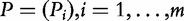, the corresponding P-values. Similarly, association of genes in G^C with the target will be represented by the vectors t^C and P^C.

In Table 1, we present competitive, self-contained and parametric methods of gene-set analysis. As we do not aim to evaluate all published methods, we only illustrate the groups by some popular or representative statistics.

Table 1:

Examples of competitive, self-contained and parametric methods

Method	Statistic	Significance assessment
Competitive with gene randomization
Q1 (Tian et al. [14])		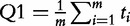Gene randomization
FCS—Functional Class Score (Pavlidis et al. [24])		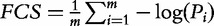Gene randomization
Competitive with sample randomization
GSEA (Subramanian et al. [1])	Kolmogorov–Smirnov statistic comparing ranks of P-values of genes in gene set versus uniform distribution	Sample randomization
GSA (Efron and Tibshirani [9])	The maxmean statistic Smax equal:	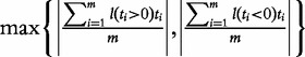Sample randomization for standardized test statistics
SAFE (Barry et al. [10])	Kolmogorov–Smirnov or Wilcoxon rank-sum statistic comparing t versus tC	Sample randomization
Self-contained
Globaltest (Goeman et al. [5])	where µ and µ2 are the are the first and second central moment of Y	Asymptotic normal distribution, or for small sample approximation by scaled χ2 distribution, or randomization of samples
Q2 (Tian et al. [14])	Same as Q1	Sample randomization
FCS.SC—self-contained version of FCS (Pavlidis et al. [24])	Same as FCS	Sample randomization
ES.SC—self-contained version of the enrichment score (Subramanian et al. [1])	Kolmogorov–Smirnov statistic comparing versus the uniform distribution	Analytical Kolmogorov–Smirnov distribution or randomization of samples
Parametric
PAGE (Kim and Volksy [15])		Null distribution of z∼N(0,1)
	where μ, δ are the mean and standard deviation of fold changes calculated for all genes, and μG is the mean of fold changes for genes in G
CATEGORY (Jiang et al. [25], Irizarry et al. [16])		Null distribution of z∼N(0,1)
Other parametric tests proposed by Irizarry et al. [16]	Wilcoxon rank-sum statistic or χ2 statistic comparing t versus tC	Corresponding analytical distributions

COMPETITIVE METHODS WITH RANDOMIZATION OF GENES OR SAMPLES

Competitive methods aim to test the null hypothesis that genes in the gene set G are at most as often differentially expressed as the genes in G^C [12]. Rejection of the hypothesis (i.e. P-value < 0.05) indicates that the gene set includes significantly more differentially expressed genes than the remaining collection of genes in the experiment, and therefore can be declared as activated.

The basic idea of these methods is well illustrated by the Q1 statistic proposed by Tian et al. [14]. The statistic aggregates the measures of association of individual genes in G with the target. Significance of the Q1 statistic is calculated by permutation of genes (rows of the matrix W), with the P-value calculated as

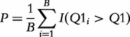(1)

where is the value of the Q1 statistic recomputed for the gene set after the ith permutation of genes, and B is the total number of permutations.

Another group of competitive methods calculate the test statistic based on X and X^C, and estimate its significance by permuting subjects (elements of Y). The most popular example is the GSEA method [1]. The statistic (enrichment score, ES) is the weighted Kolmogorov–Smirnov statistic comparing the ranks of genes in G with the uniform distribution. This is motivated by the observation that for the null hypothesis, the members of the gene set should be uniformly distributed among all the genes (all the rows of W). Significance is estimated as in Equation (1), with permutation of samples instead of genes.

Another interesting method is the GSA proposed by Efron and Tibshirani [9]. The method attempts to combine gene and sample randomization in one procedure called ‘re-standardization’. For a gene set G, the method calculates the test statistic (gene set score) S as, preferably, the maxmean statistic S_max (Table 1); however, simpler choices are also considered (such as the mean of individual gene scores in G, essentially as in the Q1 statistic). Significance is estimated using permutation of samples; however, the test statistic is standardized using gene scores calculated for all the genes in the study. Specifically, the P-value is calculated as:

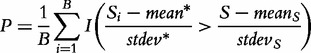(2)

where is the gene set score for the ith permutation of samples, and are the mean and standard deviation of individual gene scores for all genes in the study, and and are the mean and standard deviation of individual gene scores calculated over all genes in the study and a large number of permutations [9]. Standardization of the gene-set scores makes this method competitive, i.e. allows us to compare scores of genes in G with those outside G. Strictly, the Equation (2) is used if the test statistic S is defined as the mean gene score or mean absolute gene score. For the maxmean statistic , as defined in Table 1, the re-standardized statistic is calculated as 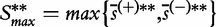, with , where is the element of the maxmean statistic calculated for the ith permutation of samples (the same re-standardization applies for ). Then the P-value is calculated as the fraction of sample permutations in which .

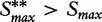SELF-CONTAINED METHODS

Self-contained methods test the null hypothesis that no genes in the gene set are associated with the target. The hypothesis is verified based on the data 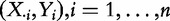while ignoring X^C.

A prominent example is the Globaltest [5] based on generalized linear model of the relationship between X and Y, with the null hypothesis assuming that all the coefficients in the model are zero. The Globaltest is derived as the score test, which guarantees high power for gene sets with many genes moderately associated with the target. Similar multivariate procedure was proposed by Mansmann and Meister [7].

Other self-contained approaches define the test statistic as the aggregate of individual gene scores (such as the Q2), with the null distribution derived by permutation of samples. Following this idea, a modification of popular competitive methods can be proposed that makes them self-contained. For instance, the FCS statistic [24] with sample-randomization null distribution becomes self-contained, and the ES statistic based on raw P-values instead of ranks also becomes self-contained.

Other self-contained approaches were proposed by Fridley et al., Dinu et al. and Kong et al. [8, 26, 27].

PARAMETRIC METHODS

Several authors criticized empirical null distribution of the GSEA or related methods and argued that simpler statistics can be used for which parametric null distributions are known. For instance, Irizarry et al. [16] proposed to directly compare the vectors of associations with the target t and t^C using more powerful tests for location and scale instead of the K–S test, with their analytical null distributions rather than empirical distributions. Similar idea was suggested by Jiang and Gentleman [25].

Another example of the parametric approach is the PAGE [15]. The method calculates the mean fold change for all genes in the experiment and compares this mean with the mean fold change for the genes in G. Under the null hypothesis, the z-score should follow the normal distribution, which is used to estimate the P-value.

MODELS OF STATISTICAL EXPERIMENT ASSUMED BY DIFFERENT METHODS

Although different in nature, virtually all methods of gene-set analysis interpret their results in terms of significance or P-values—the concepts that are meaningful in the context of statistical hypothesis testing. To correctly interpret the results, it is essential that the underlying statistical assumptions are clearly stated regarding: the null and alternative hypotheses, the sample (size and independence) and derivation of the null distribution of the test statistic. In this section, we analyse the models of statistical experiment explicitly or implicitly assumed by different gene-set analysis methods. We use here the notation introduced in the ‘Methods’ section.

Model 1

In this model, we analyse association between two random variables: , phenotype of the subject (patient), and , expression of genes in set G. We consider the experiment data X,Y as the sample of n independent realizations of these variables:

(3)

The null hypothesis assumes that and are independent.

If T is the test statistic, then the null distribution of the statistic can be non-parametrically estimated by re-calculating the statistic based on (many) samples as in Equation (3), with the values of Y randomly permuted.

It should be noted that the permutation null distribution of T is available only when can be considered independent samples from , which is not true for time-series studies.

This model of statistical experiment underlies the following gene-set analysis methods (Table 1):

• Globaltest,

• Q2,

• FCS.SC,

• ES.SC with the null distribution obtained by randomization of samples.

Indeed, these methods calculate the test statistic based on expression of genes G, , which are samples from , with significance calculated using the null distribution obtained by calculating (many) values of the statistic under permutations of sample labels. Thus, by using the sample randomization, we de facto assume the null hypothesis that expression of genes for a subject and the subject’s phenotype is independent, as stated in Model 1.

Note, however, that this model does not apply to the ES.SC when the analytical null distribution is used. Model 2 is appropriate for this case.

Model 2

In this model, we analyse association between the random variables: , phenotype of the subject, and , expression of a gene in the gene set G for the subject. We assume that expression of m genes in G measured for a subject i, denoted 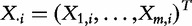, consists of m independent samples from , i.e. we assume that the genes in G are independent and governed by the same distribution.

The null hypothesis assumes that and are independent.

The experiment data X, Y represents results of m independent tests each with n samples from and :

(4)

These tests produce —m independent gene scores, i.e. measures of association between and , with their corresponding P-values .

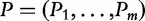Under the null hypothesis in this model, the P-values come from the Uniform(0,1) distribution. Hence, any gene-set analysis method that tests for uniformity of P_i, or for some other analytical distribution of the combination of independent t-statistics, or P-values calculated for genes in the gene set G actually realizes this model of statistical experiment. Examples of such methods include:

• ES.SC with the analytical null distribution (Table 1),

• The parametric method proposed by Irizarry et al. and Jiang and Gentleman [16, 25] (CATEGORY in Table 1),

• Fisher’s method for combining independent P-values, using the χ² null distribution [8],

• Testing for normality of t_i (as proposed by Irizarry et al. [16]).

The last two methods, suggested in literature, are not reported in Table 1.

All these methods realize Model 2, as they consider the values (or ) as independent samples from some distribution, and test whether the sample comes from the null distribution that is based on the assumption that the m tests which produced or tested independent variables: (which represent expression of a given gene in G) and (phenotype). Hence, by using this procedure to estimate significance, we de facto assume that genes in G are iid, as stated in Model 2.

Model 3

In this model, we consider the data and as iid samples drawn from two unknown distributions denoted and . Although it is hard to interpret these random variables in the context of the actual biological study, we loosely describe and as association of genes in G and outside G, respectively, with the target.

Different null hypotheses are defined in this model, e.g. that the variables and have the same distribution, or that they do not differ in some specific parameter (e.g. mean).

The gene-set analysis methods that are based on this model use different tests to compare t and t^C and different procedures to obtain the null distribution of the test statistic. Examples include (Table 1):

• Statistical tests directly comparing t and t^C (e.g. using the t-test, Wilcoxon rank-sum, χ² tests), as proposed by Irizarry et al. [16],

• PAGE [15],

• Competitive methods with gene randomization, such as the Q1 or FCS.

It should be noted that although the Q1 or FCS statistics are based only on t and do not take t^C into account, the methods are competitive because of the gene randomization procedure used to derive the null distribution. Indeed, if the gene permutation-based distribution is used as the null distribution to obtain the P-value as in Equation (1), then this is equivalent to the assumption that t and t^C have been drawn from the same distribution. Additionally, by using elements of t and elements of t^C as samples from their underlying distributions, we de facto assume that elements of t are independent, and elements of t^C are independent, which further implies independence of genes.

Model 4

In this model, we consider the experiment data Y, X and X^C as n independent realizations of the random variables , and , which represent phenotype of the subject, the subject’s expression of genes in G and expression of genes not in G:

(5)

The test statistic is calculated based on X and X^C, with its null distribution obtained by randomization of samples, as in Model 1. This procedure to obtain the null distribution implies that the actual null hypothesis assumes that and are independent and and are independent.

This model of statistical experiment is valid for competitive methods with randomization of samples, such as:

• GSEA,

• SAFE.

This model differs from Model 1 in how the test statistic is constructed: in Model 1, it is based only on X, whereas in Model 4, it includes X and X^C. Note that by permuting sample labels assigned to the data vectors , to calculate the null distribution of the test statistic, we de facto assume independence of the phenotype and genes in G and also independence of the phenotype and genes in G^C.

Finally, we want to analyse the model of statistical experiment realized by the GSA method. The method uses sample permutation test [Equation (2)] to empirically obtain the null distribution of the test statistic. Referring to Equation (2), we consider the standardized score as the test statistic, whose significance we want to obtain non-parametrically through sample permutations. Note that this statistic compares differential expression of genes in G with the mean level of differential expression observed for all genes (hence, the statistic is competitive). Significance of this statistic could be obtained by calculating many possible values of this statistic using sample permutations:

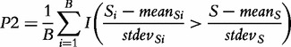(6)

where and denotes the mean and standard deviation of the gene scores over all genes calculated for the ith permutation of samples. Small P2 leads to rejection of H0 of no association of expression in subjects and their class labels, which we interpret that G is enhanced (contains more differentially expressed genes than expected by looking at the proportion of DE genes in the list of all genes), as this is what actually measures. However, we note that, strictly, the original GSA method [Equation (2)] does not produce the permutation-based null distribution of the test statistic needed to derive the P-value. Instead, the method produces the null distribution of 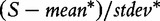, which complicates rigid interpretation of the P-value produced by Equation (2). We will return to this in ‘Empirical Comparison’ section.

VALIDITY OF THE MODELS IN THE CONTEXT OF BIOLOGICAL STUDY

Significant result (i.e. P-value P < 0.05) obtained by any gene-set analysis method means that if the actual null hypothesis of the particular method was true, then only the fraction of P repetitions of the experiment would return the data (i.e. the test statistic) more extreme than actually observed. Obviously, repetition of the experiment as perceived by the biologist consists in taking a new sample of subjects (e.g. patients) and taking a new sample of measurements from these subjects, as described in Equations (3) or (5).

The research question posed by the biologist is related to whether (i) expression of genes in G is associated with the phenotype, or (ii) frequency of differentially expressed genes in G is higher than in G^C. Question (i) is related to the self-contained null hypothesis, whereas question (ii) is related to the competitive null hypothesis, as formulated by Goeman and Buehlmann [12].

Analysing models of the statistical experiment developed in the previous section in the context of the biological experiment, we make the following observations:

1. Models 1 and 4 directly correspond to the organization of the biological experiment, where the sample [considering Model 1, Equation (3)] represents expression of m genes in G measured for n independent subjects (), together with the subjects phenotypes (). P-value P produced by tests under Model 1 have clear biological interpretation described earlier in the text, where repeating experiments can be realized by taking new samples from and , i.e. testing new patients. Significant result declared by gene-set analysis methods based on Model 1 indicates that the gene set concerned contains genes associated with the phenotype. Significant result according to Model 4 indicates that either the gene set or its complement contain genes associated with the phenotype. Hence, the methods based on Model 1 directly answer the research question (i). If we make (often reasonable) assumption that (most of) genes in G^C are not differentially expressed, then methods based on Model 4 also answer the research question (i).

2. Model 2 also closely mimics organization of the biological experiment in terms of how a sample is taken and how experiment is repeated (which is essentially done as in Model 1). However, gene-set analysis methods based on this model rely on the assumption that genes in G are independent and identically distributed—both of which seems highly unrealistic in expression studies. However, if the assumptions were true, then methods based on Model 2 would answer the research question (i).

3. Model 3 compares two samples of size m and d − m, where genes are the sampling units. In this model, we compare distributions of two unknown random variables (denoted previously and ), which produced the samples t and t^C. As we use statistical tests to compare and , we implicitly assume that elements in each of the samples t and t^C are iid, which implies that expression of genes in G are independent and identically distributed (which can be weakened for gene permutation procedures, as we only require that genes are exchangeable). The most fundamental problem with interpretation of this model is the biological meaning of the variables and . It is also not clear how repeating the biological experiment (i.e. testing new patients) could bring more samples from these variables.

In summary, only methods based on Model 1 address the research question (i), which is related to the self-contained null hypothesis. Methods based on Model 4 (this group includes popular methods such as GSEA) also address the same question, although an additional assumption is made of no association of genes outside G with the phenotype. Methods based on Model 2 also test the self-contained null hypothesis, but they make the assumption that expression of genes in G is iid. Methods based on Model 3 compare two random variables with unclear biological meaning, and, additionally, they assume that genes in G are independent and identically distributed. This leads to the conclusion that none of the methods discussed in the previous section seems to address the research question (ii), related to competitive null hypothesis, in statistically sound way.

PROPOSED INTERPRETATION OF GENE SAMPLING PROCEDURES

As the methods of gene-set analysis that use gene sampling to test the competitive null hypothesis are popular (see the review [4]), it seems compelling to find some interpretation of their results in line with the actual biological experiment.

Here, we propose such interpretation. The sample in the model is a set of n subjects. For this sample, we measure association of expression of genes in the gene set G with the phenotype, denoted t. We consider t as one realization of a random variable . In the same experiment, we measure association of genes outside G with the phenotype, denoted t^C.

We want to assess whether G is enhanced, i.e. whether genes in G are more associated with the target than the remaining genes. To do this, we randomly draw many m-element subsets from t^C, denoted tm_i, i = 1,…,B. Now we can calculate a heuristic measure of enhancement of G defined as:

(7)

where , [e.g. equals or the mean absolute value of elements of t].

Note that s intuitively addresses the question formulated in the competitive null-hypothesis, where small values of s say that it is unlikely that a randomly selected gene set of size m composed of genes from G^C realizes stronger association with the target than G, which suggests enhancement of the gene set G.

However, we should be careful not to use the language of statistical hypothesis testing while interpreting s, i.e. s is not a P-value, and s < 0.05 has nothing to do with ‘statistical significance’ of results. Result s < 0.05 means that only 5% of subsets (gene sets) of size m drawn from G^C have as extreme t values (i.e. associations with the target) as observed in G.

EMPIRICAL COMPARISON

Genes-set analysis methods based on Model 2 and 3 rely on the assumption that gene expressions are independent. In this section, we want to quantify performance of different methods if data does not follow this assumption. In the first two experiments, we focus on the self-contained hypothesis, whereas in experiments 3 and 4, we focus on the competitive hypothesis. In experiment 1, we demonstrate the false-positive rate of different methods under varying correlation of genes in the gene set. In experiment 2, we compare the power of selected methods for the cases when only a small fraction of genes in the gene set are differentially expressed. We address the criticism formulated by some authors [4] that self-contained methods may demonstrate excessive sensitivity if only a few genes in the set are associated with the target. In experiment 3, we quantify the false-positive rate of different methods under the competitive hypothesis, where many gene sets are similarly differentially expressed, but one of the gene sets contains correlated genes. In experiment 4, we compare power of different competitive methods in the setting where many gene sets are differentially expressed, but one of the gene sets is significantly more differentially expressed.

As our purpose is to compare performance of methods under known characteristics of data, we deliberately restrict this analysis to simulated data.

In experiment 1, we quantify type I error of different methods based on simple simulated data set with n = 30 samples and d = 100 or d = 1000 genes, out of which m = 40 genes constitute a gene set G. In this study, no genes in G or in G^C are differentially expressed, but genes in G are correlated. We generate expression for the genes in G from the multivariate normal distribution with the mean for each of the m genes equal 0 and the covariance matrix, which has diagonal elements equal 1 and non-diagonal elements equal r. Note that as variances of genes are 1, r is the correlation of genes in G. The remaining d − m genes come from N(0,1).

In the experiment, we vary the parameter r. We repeat the experiment 500 times and observe the P-value produced by different methods. We record how many times (out of 500) each of the methods produces significant P-value (P < 0.05), which measures the false-positive rate of each method.

Results of this study for d = 1000 are summarized in Table 2.

Table 2:

False-positive rates for the self-contained hypothesis for varying level of correlation in the gene set observed for different methods of gene set analysis

Method	Correlation r of genes in G
	0	0.2	0.4	0.6	0.8
Q1	0.05	0.096	0.178	0.22	0.282
GSEA	0.034	0.07	0.066	0.062	0.06
GSA	0.056	0.072	0.07	0.086	0.096
GSA2	0.05	0.057	0.047	0.06	0.05
SAFE	0.053	0.043	0.06	0.04	0.057
Globaltest	0.05	0.036	0.038	0.062	0.066
Q2	0.054	0.034	0.046	0.044	0.05
ES.SC	0.048	0.052	0.054	0.052	0.054
ES.SC Analytic	0.044	0.13	0.318	0.556	0.822
PAGE	0.03	0.148	0.32	0.606	0.702
CATEGORY	0.066	0.482	0.632	0.682	0.772
PAR Wilcoxon	0.056	0.516	0.644	0.716	0.802

Methods are denoted as in Table 1. The following specific settings of the methods were used: SAFE uses the Wilcoxon statistic; Globaltest uses the asymptotic null distribution; ES.SC uses null distribution based on permutation of samples; ES.SC Analytic uses the Kolmogorov–Smirnov null distribution; GSA uses all genes in the data set for re-standardization; GSA2 is the modified version of GSA with the P-value based on Equation (6). PAR Wilcoxon is the parametric method suggested by Irizarry et al. [16], see last row in Table 1.

As the gene sets contained no differentially expressed genes, the false-positive rate of 5% was expected. It can be clearly seen that the methods based on Models 2 and 3 generate excessive number of false-positive results, with the effect increasing with growing correlation between genes in G. Hence, gene sets declared as significant by these methods may only include correlated genes, with no genes associated with the target. Type I error of the methods based on Models 1 and 4 is not affected by the correlation in the gene set. We also observe that for correlated genes, the GSA method tends to produce slightly more false-positive results than expected. This may seem surprising considering the fact that the method uses sample randomization. However, the problem can be accounted for by observing that the GSA sample permutation procedure [Equation (2), valid for S being the mean gene score of the mean absolute gene score) does not actually produce the empirical null distribution of the test statistic , which is required to estimate the P-value, but rather of the quantity . The same remark is true when the maxmean is used as the test statistic (as in our simulation studies). To confirm this, we repeated the simulation with the GSA P-value calculated according to Equation (6), with the test statistic taken as the mean gene score, and observed the expected Type I error of ∼5%, whereas the original Type I error for this statistic also exceeded 5%. This modified version of the GSA based on Equation (6) is included in our simulation studies as GSA2.

We repeated the study for d = 100 and observed that Type I error decreased only for the PAGE and PAR Wilcoxon methods (e.g. the error for PAGE under correlation 0 to 0.8 decreased to 0.008, 0.052, 0.154, 0.368, 0.568, respectively). For all the other methods, Type I error is not affected by the total number of genes d.

In experiment 2, we assume that n.DE out of m genes in G is differentially expressed and correlated. We divide the samples into two groups of 15 samples and generate expression of the n.DE genes in the first group from the multivariate normal distribution with the mean 0, and in the second group with the mean equal Δ. The covariance matrix for both groups has diagonal elements equal 1 and non-diagonal elements equal r. The remaining m − n.DE genes in G and the d − m genes in G^C are not correlated and not differentially expressed and come from N(0,1).

In this study, we compare the power of different methods as a function of the number of differentially expressed genes (n.DE = 2, 5, 10, 40), the effect strength (Δ = 0.5, 1, 1.5) and correlation r. We measure power as the fraction of replications of the experiment, which produce P-value < 0.05, i.e. declare the gene set as significant.

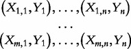
Results are summarized in Figures 1–3.

Figure 1:

Power of selected methods as a function of correlation and the number of differentially expressed genes (n.DE) in the gene set. Small effect, Δ = 0.5. Number of genes d = 1000.

Figure 2:

Power of selected methods as a function of correlation and the number of differentially expressed genes (n.DE) in the gene set. Medium effect, Δ = 1. Number of genes d = 1000.

Figure 3:

Power of selected methods as a function of correlation and the number of differentially expressed genes (n.DE) in the gene set. Strong effect, Δ = 1.5. Number of genes d = 1000.

We focus only on the methods that use sample randomization: Globaltest, FCS.SC, ES.SC (methods based on Model 1), GSEA, SAFE (methods based on Model 4) and GSA. We do not consider methods based on gene randomization or parametric models (i.e. methods based on Models 2 and 3), as they tend to produce excessive number of false-positive results from data with only correlated but no differentially expressed genes.

It can be clearly seen that if only a small fraction of genes in the gene set is associated with the phenotype, then the methods considerably differ in power, with the Globaltest, GSEA and GSA consistently showing higher power than the remaining methods (e.g. Figure 3, bottom right panel). We also observe that for small effect (Figure 1), GSA demonstrates slightly better power than other methods, whereas for medium (Figure 2) and strong effects (Figure 3), the Globaltest outperforms other methods. Our study also confirms that the Globaltest tends to declare as significant the gene sets with few differentially expressed genes with strong effect (Figure 3, bottom left panel). This high power is not necessarily a desirable feature, if the purpose of analysis is to find gene sets with moderate, but consistent, effect observed over many genes. Finally, we observed sensitivity of the results to the total number of genes d. In Figure 4, we compare power of competitive methods for d = 1000 and d = 100 (we omit the self-contained methods, as their power is obviously not affected by d). We observe that increasing d (with m fixed) leads to higher power of competitive methods.

Figure 4:

Power of sample randomization, competitive methods for different number of genes in the study d = 100 or d = 1000, as a function of correlation and the number of differentially expressed genes (n.DE) in the gene set. Medium effect, Δ = 1.

In experiment 3, we analyse the type I error under the competitive hypothesis. We focus here only on competitive or parametric methods that compare expression in G and in G^C, such as Q1, GSA, GSA2, GSEA, SAFE, PAGE and PAR Wilcoxon (Tables 1 and 2). We generated data with 30 samples divided into two groups of 15 samples, and 1000 genes divided into 50 gene sets each with 20 genes. We generated expression of all the genes from N(0,1), then in 30% randomly selected genes we added Δ = 1 in the second group of samples. Hence, all the gene sets contained on average 30% (i.e. n.DE = 6) differentially expressed genes. In the first gene set (GS1), we allowed for correlation among the genes (i.e. expression in GS1 was generated from the multivariate normal distribution, as in the second experiment, with the effect size Δ = 1 and n.DE = 6). In this study, we varied the correlation in GS1. We repeated the experiment 200 times and reported the fraction of replications of the experiment that produced P-value < 0.05 for GS1, i.e. declared the first gene set as significant in comparison with the remaining sets. This measures the type I error of the methods. Results for 30% (n.DE = 6) and 60% (n.DE = 12) differentially expressed genes in all gene sets are summarized in Table 3. We observe that for uncorrelated genes in GS1, all the methods (with the exception of GSEA) control the type I error. However, correlated genes lead to increased type I error for the gene randomization (Q1) and parametric methods (PAGE and PAR Wilcoxon).

Table 3:

False-positive rates for the competitive hypothesis as a function of the average number of differentially expressed genes in all the gene sets (n.DE) and correlation in GS1

Method	n.DE	Correlation r of genes in GS1
		0	0.2	0.4	0.6	0.8
Q1	6	0.005	0.01	0.055	0.035	0.095
GSEA		0.15	0.205	0.155	0.175	0.16
GSA		0.01	0.01	0.005	0	0.005
GSA2		0.01	0	0	0.005	0
SAFE		0.01	0.01	0	0	0
PAGE		0	0.005	0.035	0.045	0.09
PAR Wilcoxon		0.005	0	0.02	0.01	0.01
Q1	12	0.01	0.065	0.09	0.115	0.175
GSEA		0.04	0.085	0.075	0.09	0.075
GSA		0.02	0.02	0.005	0.03	0.005
GSA2		0	0.02	0.025	0.02	0.01
SAFE		0.005	0.01	0.01	0.025	0.035
PAGE		0.005	0.07	0.15	0.26	0.285
PAR Wilcoxon		0.005	0.02	0.115	0.175	0.245

In experiment 4, we want to compare power of different methods when the data contains many differentially expressed gene sets, with some of the gene sets significantly more differentially expressed. We focus here only on the methods analysed in experiment 3. We used the same data as in experiment 3 with 30% of differentially expressed genes in the gene sets 2 through 50; however, we varied the number of differentially expressed genes in GS1 (n.DE = 6, 12, 18). We repeated the experiment 200 times and reported the fraction of replications of the experiment, which produced P-value < 0.05 for GS1, i.e. declared the first gene set as significant in comparison with the remaining sets (we refer to this as ‘power’ of the methods). Results are summarized in Figure 5. We observe that for n.DE = 6, the GS1 is not regarded as significantly enriched by most of the methods, even if the differentially expressed genes are correlated. Only the GSEA tends to declare GS1 as significant (in 10–20% replications of the experiment), as it probably measures both association with the target and enrichment. As expected, with increasing n.DE, the methods recognize GS1 as enriched; however, in our study, GSEA seems to have highest power (Figure 5, bottom left panel). Interestingly, if the differentially expressed genes are correlated, GSA, GSEA and SAFE seem to lose power. We observe that GSA2 [the modified version of GSA based on Equation (6)] generally realized higher power than the original GSA. To illustrate peculiarities of some test statistics, we also demonstrated the case where the gene set of interest contains fewer genes associated with the target then the remaining gene sets (point n.DE = 0 in Figure 5). We observe that PAGE, SAFE and PAR Wilcoxon (proposed by Irizarry et al. [16]) declare GS1 as significant, although it contains no differentially expressed genes. Clearly, these methods signal that the pattern of expression in the gene set is different than in the remaining sets, and not necessarily that the gene set is enhanced.

Figure 5:

Power of methods comparing expression in GS1 with expression in the remaining gene sets as a function of the number of differentially expressed genes in GS1 (n.DE) and their correlation.

CONCLUSION

In this article, we analysed the models of statistical experiment that underlie commonly used methods of gene-set analysis. We showed that only the self-contained methods and competitive methods that use sample randomization to generate the null distribution are based on the models of experiment that closely follow organization of the actual biological study. Thus, these methods produce statistically sound results, albeit under slightly different null hypotheses. Other gene-set analysis methods, those based on simplifying parametric assumptions or on gene randomization, either rely on unrealistic assumptions pertaining to distribution of genes or, additionally, compare random variables, whose biological interpretation is unclear. We must also note that popular competitive methods (such as GSEA or SAFE) do not, strictly, test the competitive null hypothesis, as formulated by Goeman et al. A significant result from these methods does not necessarily mean that the gene set of interest contains more genes associated with the phenotype than its complement, but it rather means that either the gene set or its complement are associated with the phenotype.

Although we do not want to recommend one, best method of gene set analysis, based on this work we could suggest the Globaltest, GSA or GSEA as the preferable tools for gene-set analysis studies. These methods produce biologically interpretable P-values and realize higher power than other sample-randomization methods compared in this article. We observe, however, that significant results from the Globaltest may be because of only a few genes strongly associated with the target. GSA or GSEA methods seem to be less powerful for such data, which seems to be an advantage of these methods.

Finally, we want to point that when comparing results produced by different methods or considering the application of some methods, it seems advisable to consider the actual statistical model implied by the method, as small P-values produced by gene-randomization or parametric methods do not necessarily imply that the gene set is enhanced.

Key Points.

• Out of the vast collection of gene-set analysis approaches, only the self-contained methods and competitive methods that use sample randomization to generate the null distribution are based on the models of experiment, which closely follow organization of the actual biological study.

• Popular competitive methods (such as GSEA or SAFE) do not test the competitive null hypothesis, as formulated by Goeman et al. A significant result from these methods does not necessarily mean that the gene set of interest contains more genes associated with the phenotype than its complement, but it rather means that either the gene set or its complement are associated with the phenotype.

• Competitive methods that use gene randomization can produce biologically meaningful results, although the results cannot be formulated using the concept of statistical significance or a P-value. A heuristic measure of similarity of differential expression patterns in the gene set and its complement can be used instead.

FUNDING

National Science Centre of Poland (grant N516 510239).

Biography

Henryk Maciejewski is an assistant professor at the Institute of Computer Engineering, Control and Robotics of the Wroclaw University of Technology. His research interests are mainly in machine learning and bioinformatics.

References

- 1.Subramanian A, Tamayo P, Mootha VK, et al. Gene set enrichment analysis: a knowledge-based approach for interpreting genome-wide expression profiles. Proc Natl Acad Sci USA. 2005;102(43):15545–50. doi: 10.1073/pnas.0506580102. [DOI] [PMC free article] [PubMed] [Google Scholar]
- 2.Ein-Dor L, Kela I, Getz G, et al. Outcome signature genes in breast cancer: is there a unique set? Bioinformatics. 2005;21(2):171–8. doi: 10.1093/bioinformatics/bth469. [DOI] [PubMed] [Google Scholar]
- 3.Ein-Dor L, Yuk O, Domany E. Thousands of samples are needed to generate a robust gene list for predicting outcome of cancer. Proc Natl Acad Sci USA. 2006;103(15):5923–28. doi: 10.1073/pnas.0601231103. [DOI] [PMC free article] [PubMed] [Google Scholar]
- 4.Nam D, Kim SY. Gene-set approach for expression pattern analysis. Brief Bioinform. 2008;9(3):189–97. doi: 10.1093/bib/bbn001. [DOI] [PubMed] [Google Scholar]
- 5.Goeman JJ, van de Geer SA, de Kort F, et al. A global test for groups of genes: testing association with clinical outcome. Bioinformatics. 2004;20(1):93–9. doi: 10.1093/bioinformatics/btg382. [DOI] [PubMed] [Google Scholar]
- 6.Goeman JJ, Oosting J, Cleton-Jansen AM, et al. Testing association of a pathway with survival using gene expression data. Bioinformatics. 2005;21(9):1950–7. doi: 10.1093/bioinformatics/bti267. [DOI] [PubMed] [Google Scholar]
- 7.Mansmann U, Meister R. Testing differential gene expression in functional groups—Goeman’s global test versus an ANCOVA approach. Methods Inf Med. 2005;44:449–53. [PubMed] [Google Scholar]
- 8.Fridley BL, Jenkins GD, Biernacka JM. Self-contained gene-set analysis of expression data: an evaluation of existing and novel methods. PLoS One. 2010;5(9):e12693. doi: 10.1371/journal.pone.0012693. [DOI] [PMC free article] [PubMed] [Google Scholar]
- 9.Efron B, Tibshirani R. On testing the significance of sets of genes. Ann Appl Stat. 2007;1(1):107–29. [Google Scholar]
- 10.Barry WT, Nobel AB, Wright FA. Significance analysis of functional categories in gene expression studies: a structured permutation approach. Bioinformatics. 2005;21(9):1943–9. doi: 10.1093/bioinformatics/bti260. [DOI] [PubMed] [Google Scholar]
- 11.Newton MA, Quintana FA, den Boon JA. Random set methods identify distinct aspects of the enrichment signal in gene-set analysis. Ann Appl Stat. 2007;1(1):85–106. [Google Scholar]
- 12.Goeman JJ, Buehlmann P. Analyzing gene expression data in terms of gene sets: methodological issues. Bioinformatics. 2007;23(8):980–7. doi: 10.1093/bioinformatics/btm051. [DOI] [PubMed] [Google Scholar]
- 13.Pavlidis P, Lewis DP, Noble WS. Exploring gene expression data with class scores. Pac Symp Biocomput. 2002;7:474–85. [PubMed] [Google Scholar]
- 14.Tian L, Greenberg SA, Kong SW, et al. Discovering statistically significant pathways in expression profiling studies. Proc Natl Acad Sci USA. 2005;102(38):13544–9. doi: 10.1073/pnas.0506577102. [DOI] [PMC free article] [PubMed] [Google Scholar]
- 15.Kim SY, Volsky DJ. PAGE: parametric analysis of gene set enrichment. BMC Bioinformatics. 2005;6:144. doi: 10.1186/1471-2105-6-144. [DOI] [PMC free article] [PubMed] [Google Scholar]
- 16.Irizarry RA, Wang C, Zhou Y, et al. Gene set enrichment analysis made simple. Stat Methods Med Res. 2009;18(6):565–75. doi: 10.1177/0962280209351908. [DOI] [PMC free article] [PubMed] [Google Scholar]
- 17.Liu Q, Dinu I, Adewale AJ, et al. Comparative evaluation of gene set analysis methods. BMC Bioinformatics. 2007;8:431. doi: 10.1186/1471-2105-8-431. [DOI] [PMC free article] [PubMed] [Google Scholar]
- 18.Song S, Black MA. Microarray-based gene set analysis: a comparison of current methods. BMC Bioinformatics. 2008;9:502. doi: 10.1186/1471-2105-9-502. [DOI] [PMC free article] [PubMed] [Google Scholar]
- 19.Dinu I, Liu Q, Potter JD, et al. A biological evaluation of six gene set analysis methods for identification of differentially expressed pathways in microarray data. Cancer Inform. 2008;6:357–68. doi: 10.4137/cin.s867. [DOI] [PMC free article] [PubMed] [Google Scholar]
- 20.Wu MC, Lin X. Prior biological knowledge-based approaches for the analysis of genome-wide expression profiles using gene sets and pathways. Stat Methods Med Res. 2009;18(6):577–93. doi: 10.1177/0962280209351925. [DOI] [PMC free article] [PubMed] [Google Scholar]
- 21.Ackermann M, Strimmer K. A general modular framework for gene set enrichment analysis. BMC Bioinformatics. 2009;10:47. doi: 10.1186/1471-2105-10-47. [DOI] [PMC free article] [PubMed] [Google Scholar]
- 22.Hung JH, Yang TH, Hu Z, et al. Gene set enrichment analysis: performance evaluation and usage guidelines. Brief Bioinform. 2012;13(3):281–91. doi: 10.1093/bib/bbr049. [DOI] [PMC free article] [PubMed] [Google Scholar]
- 23.Mootha VK, Lindgren CM, Eriksson KF, et al. PGC-1α-responsive genes involved in oxidative phosphorylation are coordinately downregulated in human diabetes. Nat Genet. 2003;34:267–73. doi: 10.1038/ng1180. [DOI] [PubMed] [Google Scholar]
- 24.Pavlidis P, Qin J, Arango V, et al. Using the gene ontology for microarray data mining: a comparison of methods and application to age effect in human prefrontal cortex. Neurochem Res. 2004;29(6):1213–22. doi: 10.1023/b:nere.0000023608.29741.45. [DOI] [PubMed] [Google Scholar]
- 25.Jiang Y, Gentleman R. Extensions to gene set enrichment. Bioinformatics. 2007;23(3):306–13. doi: 10.1093/bioinformatics/btl599. [DOI] [PubMed] [Google Scholar]
- 26.Dinu I, Potter JD, Mueller T, et al. Improving gene set analysis of microarray data by SAM-GS. BMC Bioinformatics. 2007;8:242. doi: 10.1186/1471-2105-8-242. [DOI] [PMC free article] [PubMed] [Google Scholar]
- 27.Kong SW, Pu WT, Park PJ. A multivariate approach for integrating genome-wide expression data and biological knowledge. Bioinformatics. 2006;22(19):2373–80. doi: 10.1093/bioinformatics/btl401. [DOI] [PMC free article] [PubMed] [Google Scholar]